Non-linear vibration of Euler-Bernoulli beams
Abstract
In this paper, variational iteration (VIM) and parametrized perturbation (PPM) methods have been used to investigate non-linear vibration of Euler-Bernoulli beams subjected to the axial loads. The proposed methods do not require small parameter in the equation which is difficult to be found for nonlinear problems. Comparison of VIM and PPM with Runge-Kutta 4th leads to highly accurate solutions. Keywords
Variational Iteration Method (VIM), Parametrized Pertur-bation Method (PPM), Galerkin method, non-linear vibra-tion, Euler-Bernoulli beam.
A.Bararia,∗
, H.D. Kalijib,
M. Ghadimic and G. Domairryc
a
Department of Civil Engineering, Aalborg University, Sohng˚ardsholmsvej 57, 9000 Aalborg, Aalborg – Denmark
b
Department of Mechanical Engineering, Islamic Azad University, Semnan Branch, Semnan – Iran
c
Department of Mechanical Engineering, Babol University of Technology, Babol – Iran
Received 25 Oct 2010; In revised form 22 Feb 2011
∗Author email: [email protected]
1 INTRODUCTION
The demand for engineering structures is continuously increasing. Aerospace vehicles, bridges, and automobiles are examples of these structures. Many aspects have to be taken into consider-ation in the design of these structures to improve their performance and extend their life. One aspect of the design process is the dynamic response of structures. The dynamics of distributed-parameter and continuous systems, like beams, were governed by linear and nonlinear partial-differential equations in space and time. It was difficult to find the exact or closed-form solu-tions for nonlinear problems. Consequently, researchers were used two classes of approximate solutions of initial boundary-value problems: numerical techniques [28, 31], and approximate analytical methods [2, 26]. For strongly non-linear partial-differential, direct techniques, such as perturbation methods, were not utilized to solve directly the non-linear partial-differential equations and associated boundary conditions. Therefore first partial-differential equations are discretized into a set of non-linear ordinary-differential equations using the Galerkin approach and the governing problems are then solved analytically in time domain.
Max-Min [15, 19, 29], Differential Transform Method [16], Adomian Decomposition Method [22], Energy Balance [23, 30], etc.
Kopmaz et al. [20] considered different approaches to describing the relationship between the bending moment and curvature of an Euler-Bernoulli beam undergoing a large deforma-tion. Then, in the case of a cantilevered beam subjected to a single moment at its free end, the difference between the linear and the nonlinear theories based on both the mathematical curvature and the physical curvature was shown. Biondi and Caddemi [8] studied the problem of the integration of the static governing equations of the uniform Euler-Bernoulli beams with discontinuities, considering the flexural stiffness and slope discontinuities.
The vibration problems of uniform Euler- Bernoulli beams can be solved by analytical or approximate approaches [10, 21]. Pirbodaghi et al. [25] studied non-linear vibration behaviour of geometrically non-linear Euler-Bernoulli beams subjected to axial loads using homotopy analysis method. Also, the effect of vibration amplitude on the non-linear frequency and buckling load is discussed. Burgreen [9] investigated the free vibrations of a simply supported buckled beam using a single-mode discretization. He pointed out the natural frequencies of buckled beams depend on the amplitude of vibration. Eisley [11, 12] used a single-mode discretization to investigate the forced vibrations of buckled beams and plates. He considered both simply supported and clamped-clamped boundary conditions. For a clamped-clamped buckled beam, Eisley [11, 12] used the first buckling mode in the discretization procedure. He obtained similar forms of the governing equations for simply supported and clamped-clamped buckled beams.
The main purpose of this study is to obtain the analytical expression for geometrically non-linear vibration of clamped-clamped Euler-Bernoulli beams fixed at one end. Geometric non-linearity arises from non-linear strain-displacement relationships. This type of nonlinearity is most commonly treated in the literature. Sources of this type of nonlinearity include mid-plane stretching, large curvatures of structural elements, and large rotation of elements. First, the governing non-linear partial differential equation using Galerkin method was reduced to a single non-linear ordinary differential equation. It was then assumed that only fundamental mode was excited. The later equation was solved analytically in time domain using VIM and PPM. Ultimately, VIM and PPM methods are compared with Runge-Kutta 4th method.
2 DESCRIPTION OF THE PROBLEM
Consider a straight beam on an elastic foundation with length L, a cross-section A, a mass per unit lengthµ, moment of inertiaI, and modulus of elasticityE that subjected to an axial
consequently the rotation of the cross section is due to bending only. The last assumption, which is called the incompressibility condition, assumes no transverse normal strains. The last two assumptions are the basis of the Euler-Bernoulli beam theory [27].
The equation of motion including the effects of mid-plane stretching is given by:
EI∂ 4˜
W ∂X˜4 +µ
∂2W˜ ∂˜t2 +F˜
∂2W˜ ∂X˜2 +C
∂W˜ ∂˜t +
˜
KW˜ −EA 2L
∂2W˜ ∂X˜2 ∫
L
0 ( ∂W˜
∂X˜ ) 2
dX˜ =U(X,˜ t˜) (1)
Where C is the viscous damping coefficient, ˜Kis a foundation modulus and U is a dis-tributed load in the transverse direction.
Figure 1 A schematic of an Euler-Bernoulli beam subjected to an axial load.
Assume the non-conservative forces were equal to zero. Therefore Eq. (1) can be written as follows:
EI∂ 4˜
W
∂X˜4 +µ ∂2 ˜
W ∂t˜2 +
˜
F∂ 2˜
W
∂X˜2 +
˜
KW˜ −EA
2L ∂2˜
W
∂X˜2 ∫ L
0 ( ∂W˜
∂X˜ ) 2
dX˜ =0. (2)
For convenience, the following non-dimensional variables are used:
X= X˜
L, W =
˜
W
R, t=t˜
√
EI
µL4, F =
˜
F L2
EI , K=
˜
KL4
EI . (3)
Where R=(I/A)0.5 is the radius of gyration of the cross-section. As a result, Eq. (2) can be written as follows:
∂4 W ∂X4 +
∂2 W ∂t2 +F
∂2 W
∂X2 +KW−
1 2
∂2 W ∂X2 ∫
1
0 ( ∂W ∂X)
2
dX=0. (4)
Assuming W(X, t)=φ(X)ψ(t)whereφ(X)is the first eigenmode of the beam [32] and ap-plying the Galerkin method, the equation of motion is obtained as follows:
¨
Where α=α1+α2F+K andα1, α2and β are as follows:
α1= ∫ 1
0 φ ivφdx
∫01φ
2dx , α2= ∫01φ
′′
φdx
∫01φ
2dx , β=
−0.5∫
1
0 (φ
′′
∫01φ
′2
dx)φdx
∫01φ
2dx (6)
The Eq. (5) is the governing non-linear vibration of Euler-Bernoulli beams. The center of the beam subjected to the following initial conditions:
ψ(0)=A, ψ˙(0)=0 (7)
where Adenotes the non-dimensional maximum amplitude of oscillation.
3 BASIC IDEA OF VARIATIONAL ITERATION METHOD
To illustrate the basic concepts of the VIM, we consider the following differential equation:
Lu+N u=g(t). (8)
Where L is a linear operator, N a nonlinear operator and g(t) an inhomogeneous term. According to VIM, we can write down a correction functional as follows:
un+1(t)=un(t)+∫ t
0
λ(Lun(η)+Nu˜n(η)−g(η))dη. (9)
Where λ is a general Lagrange multiplier which can be identified optimally via the varia-tional theory [17]. The subscript n indicates the nth approximation and ˜un is considered as a
restricted variation [17], i.e. δu˜n=0.
4 APPLICATION OF VARIATIONAL ITERATION METHOD
To solve Eq. (5) by means of VIM, we start with an arbitrary initial approximation:
ψ0=Acos(ωt). (10)
From Eq. (5), we have:
¨
ψ=−αψ−βψ3 ⇒ ψ¨=−αAcos(ωt)−βA 3
cos3
(ωt). (11) Integrating twice yields:
ψ1= −9αA−7βA 3
+9αAcos(ωt)+βA3cos3(ωt)+6βA3cos(ωt)
9ω2 . (12)
Equating the coefficients of cos(ωt) inψ0 and ψ1, we have:
ωV IM =
√
And therefore,
ψ0=Acos(√α+0.75βA2t). (14)
Where δu˜n=0 is considered as restricted variation.
ψn+1(t)=ψn(t)+∫ t
0 λ( d2
ψn
dη2 +αψn+βψ 3
n)dη. (15)
Its stationary conditions can be obtained as follows:
1−λ′∣η=t =0, (16)
λ∣η=t =0, (17)
λ′′
+ω2λ=0. (18)
Therefore, the multiplier, can be identified as
λ=
1
ωsinω(η−t). (19)
As a result, we obtain the following iteration formula:
ψn+1(t)=ψn(t)+∫ t
0 (
1
ωsinω(η−t)).( d2
ψn
dη2 +αψn+βψ 3
n)dη. (20)
By the iteration formula (20), we can directly obtain other components as:
ψ1(t)=Acos(ω t)−A 3
βcos(ω t)−(16ω2
−16α−12A2β)Aω tsin(ω t)−A3βcos(3ω t)
32ω2 . (21)
Where ω is evaluated from Eq. (13).
In the same manner, the rest of the components of the iteration formula can be obtained.
5 APPLICATION OF PARAMETRIZED PERTURBATION METHOD
Equation of motion, which reads:
¨
ψ(t)+αψ(t)+βψ(3t)=0, ψ(0)=A, ψ˙(0)=0. (22)
We let
ψ=εU, (23)
¨
U +α U+ε2β U3=0, U(0)=A/ε, U˙(0)=0. (24)
We suppose that the solution of Eq. (24) and the constant α, can be expressed in the forms:
U =U0+ε2U1+ε4U2+ε6U3+... (25)
α=ω2+ε2ω1+ε4ω2+ε6ω3+... (26)
Substituting Eqs. (25) and (26) into Eq. (24) and equating coefficients of same powers of
εyields the following equations:
¨
U0+ω2U0=0, U0(0)=A/ε, U0˙ (0)=0. (27)
¨
U1+ω2U1+ω1U0+βU03=0, U1(0)=0, U1˙ (0)=0. (28)
Solving Eq. (27) we obtain:
U0= A
ε cos(ω t). (29)
Therefore, Eq. (28) can be re-written as:
¨
U1+ω2U1+(ω1+3βA 2
4ε2 ) A
ε cos(ω t)+ βA3
4ε3 cos(3ω t)=0. (30)
Avoiding the presence of a secular terms needs:
ω1=−3βA
2
4ε2 . (31)
Substituting Eq. (31) into Eq. (26)
ωP P M =
√
α+0.75βA2.
(32)
Solving Eq. (30), we obtain:
U1=− A 3
β
32ω2ε3(cos(ω t)−cos(3ω t)). (33)
Its first-order approximation is sufficient, and then we have:
ψ=εU =ε(U0+ε2U1)=Acos(ω t)− A 3
β
32ω2[cos(ω t)−cos(3ω t)]. (34)
6 RESULTS AND DISCUSSIONS
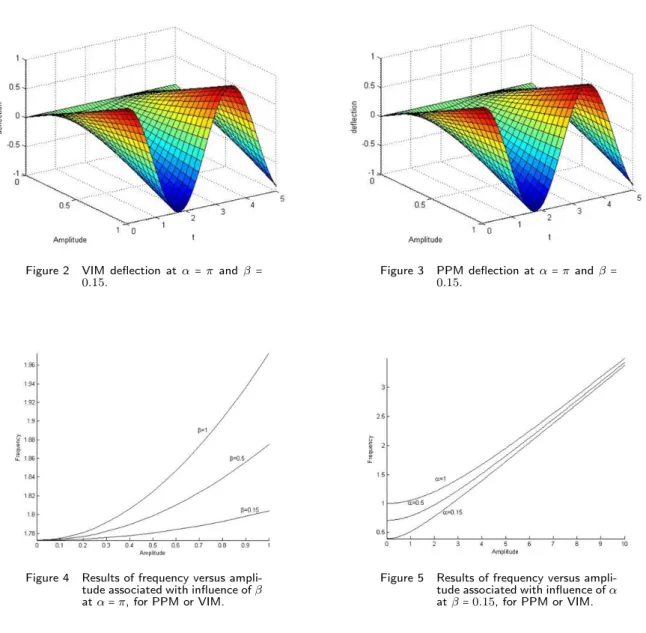
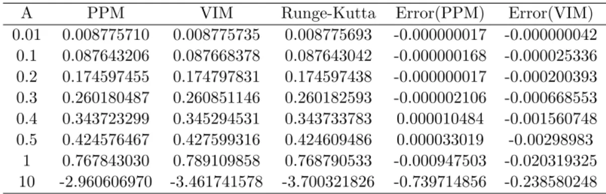
The behavior ofψ(A, t) obtained by VIM and PPM at α=π and β=0.15 is shown in Figs. 2 and 3. Influence of coefficientsβ and αon frequency and amplitude has been investigated and plotted in Figs. 4 and 5, respectively. The comparison of the dimensionless deflection versus time for results obtained from VIM, PPM and Runge-Kutta 4th order has been depicted in Fig. 6 for α=π and β =0.15, with maximum deflection at the center of the beam equal to five (A=5). The solutions are also compared for t=0.5 in Table 1. It can be observed that there is an excellent agreement between the results obtained from VIM and PPM with those of Runge-Kutta 4th order method [1].
Figure 2 VIM deflection atα=π and β=
0.15. Figure 3 PPM deflection at0.15. α=π andβ=
Figure 4 Results of frequency versus ampli-tude associated with influence ofβ
atα=π, for PPM or VIM.
Figure 5 Results of frequency versus ampli-tude associated with influence ofα
Figure 6 Results comparison between VIM and PPM deflection versus time atα=π,β=0.15andA=5with
Runge-Kutt 4th order.
Table 1 Comparison between PPM & VIM with time marching solution for the motion equation (4), when
t=0.5(s),α=1andβ=1.
A PPM VIM Runge-Kutta Error(PPM) Error(VIM) 0.01 0.008775710 0.008775735 0.008775693 -0.000000017 -0.000000042
0.1 0.087643206 0.087668378 0.087643042 -0.000000168 -0.000025336 0.2 0.174597455 0.174797831 0.174597438 -0.000000017 -0.000200393 0.3 0.260180487 0.260851146 0.260182593 -0.000002106 -0.000668553 0.4 0.343723299 0.345294531 0.343733783 0.000010484 -0.001560748 0.5 0.424576467 0.427599316 0.424609486 0.000033019 -0.00298983
1 0.767843030 0.789109858 0.768790533 -0.000947503 -0.020319325 10 -2.960606970 -3.461741578 -3.700321826 -0.739714856 -0.238580248
7 CONCLUSIONS
References
[1] D. A. Anderson and J.C. Tannehill. Computational Fluid Mechanics and Heat Transfer. Hemisphere Publishing Corp, 1984.
[2] L. Azrar, R. Benamar, and R.G. White. A semi-analytical approach to the non-linear dynamic response problem of S-S and C-C beams at large vibration amplitudes part I: general theory and application to the single mode approach to free and forced vibration analysis. J. Sound Vib., 224:183–207, 1999.
[3] A. Barari, B. Ganjavi, M. Ghanbari Jeloudar, and G. Domairry. Assessment of two analytical methods in solving the linear and nonlinear elastic beam deformation problems. Journal of Engineering, Design and Technology, 8(2):127– 145, 2010.
[4] A. Barari, A. Kimiaeifar, G. Domairry, and M. Moghimi. Analytical evaluation of beam deformation problem using approximate methods. Songklanakarin Journal of Science and Technology, 32(3):207–326, 2010.
[5] A. Barari, M. Omidvar, D.D. Ganji, and A. Tahmasebi Poor. An approximate solution for boundary value problems in structural engineering and fluid mechanics. Journal of Mathematical Problems in Engineering, pages 1–13, 2008. Article ID 394103.
[6] A. Barari, M. Omidvar, Abdoul R. Ghotbi, and D.D. Ganji. Application of homotopy perturbation method and variational iteration method to nonlinear oscillator differential equations.Acta Applicandae Mathematicae, 104:161– 171, 2008.
[7] M. Bayat, M. Shahidi, A. Barari, and G. Domairry. On the approximate analysis of nonlinear behavior of structure under harmonic loading. International Journal of Physical Sciences, 5(7):1074–1080, 2010.
[8] B. Biondi and S. Caddemi. Closed form solutions of euler-bernoulli beams with singularities. International Journal of Solids and Structures, 42:3027–3044, 2005.
[9] D. Burgreen. Free vibration of a pin-ended column with constant distance between pin ends. Journal of Applied Mechanics, 18:135–139, 1984.
[10] A. Dimarogonas. Vibration for engineers. Prentice-Hall, Inc., 2nd edition, 1996.
[11] J. G. Eisley. Large amplitude vibration of buckled beams and rectangular plates.AIAA Journal, 2:2207–2209, 1964.
[12] J. G. Eisley. Nonlinear vibration of beams and rectangular plates. ZAMP, 15:167–175, 1964.
[13] A. Fereidoon, M. Ghadimi, A. Barari, H.D. Kaliji, and G. Domairry. Nonlinear vibration of oscillation systems using frequency-amplitude formulation. Shock and Vibration, 2011. DOI: 10.3233/SAV-2011-0633.
[14] F. Fouladi, E. Hosseinzadeh, A. Barari, and G. Domairry. Highly nonlinear temperature dependent fin analysis by Variational Iteration Method.Journal of Heat Transfer Research, 41(2):155–165, 2010.
[15] S.S. Ganji, A. Barari, and D.D. Ganji. Approximate analyses of two mass-spring systems and buckling of a column.
Computers & Mathematics with Applications, 61(4):1088–1095, 2011.
[16] S.S. Ganji, A. Barari, L.B. Ibsen, and G. Domairry. Differential transform method for mathematical modeling of jamming transition problem in traffic congestion flow.Central European Journal of Operations Research, 2011. DOI: 10.1007/s10100-010-0154-7.
[17] J.H. He. Variational iteration method – a kind of non-linear analytical technique: Some examples. International Journal of Nonlinear Mechanics, 34:699–708, 1999.
[18] J.H. He. Some asymptotic methods for strongly nonlinear equations. International Journal of Modern Physics B, 20(10):1141–1199, 2006.
[19] L.B. Ibsen, A. Barari, and A. Kimiaeifar. Analysis of highly nonlinear oscillation systems using He’s max-min method and comparison with homotopy analysis and energy balance methods. Sadhana, 35:1–16, 2010.
[20] O. Kopmaz and ¨O. G¨undogdu. On the curvature of an euler-bernoulli beam. International Journal of Mechanical Engineering Education, 31:132–142, 2003.
[21] L. Meirovitch. Fundamentals of vibrations. McGraw-Hill, 2001. International Edition.
[23] M. Momeni, N. Jamshidi, A. Barari, and D.D. Ganji. Application of He’s energy balance method to Duffing harmonic oscillators.International Journal of Computer Mathematics, 88(1):135–144, 2011.
[24] M. Omidvar, A. Barari, M. Momeni, and D.D. Ganji. New class of solutions for water infiltration problems in unsaturated soils.Geomechanics and Geoengineering: An International Journal, 5:127–135, 2010.
[25] T. Pirbodaghi, M.T. Ahmadian, and M. Fesanghary. On the homotopy analysis method for non-linear vibration of beams.Mechanics Research Communications, 36:143–148, 2009.
[26] M.I. Qaisi. Application of the harmonic balance principle to the nonlinear free vibration of beams. Appl. Acoust., 40:141–151, 1993.
[27] S. S. Rao. Vibraton of Continuous Systems. John Wiley & Sons, Inc., Hoboken, New Jersey, 2007.
[28] B.S. Sarma and T.K. Varadan. Lagrange-type formulation for finite element analysis of nonlinear beam vibrations.
J. Sound Vib., 86:61–70, 1983.
[29] M. G. Sfahani, S.S. Ganji, A. Barari, H. Mirgolbabaei, and G. Domairry. Analytical solutions to nonlinear conservative oscillator with fifth-order non-linearity.Earthquake Engineering and Engineering Vibration, 9(3):367–374, 2010.
[30] M.G. Sfahani, A. Barari, M. Omidvar, S.S. Ganji, and G. Domairry. Dynamic response of inextensible beams by improved Energy Balance Method. InProceedings of the Institution of Mechanical Engineers, Part K: Journal of Multi-body Dynamics., volume 225(1), pages 66–73, 2011.
[31] Y. Shi and C.A. Mei. Finite element time domain model formulation for large amplitude free vibrations of beams and plates.J. Sound Vib., 193:453–465, 1996.