249 DOI: 10.21279/1454-864X-16-I1-043
© 2015. This work is licensed under the Creative Commons Attribution-Noncommercial-Share Alike 4.0 License.
CONSIDERATIONS REGARDING THE NORMAL STRESS (X AXIS) DEVELOPED ON A
2000X100X4MM PLATE DURING THE IMPACT WITH A 6.2KG CYLINDRICAL BODY
Adrian POPA1 Marian RISTEA2
Ionut-Cristian SCURTU3 Daniel MARASESCU4
1Assist prof. PhD Eng. “Mircea cel Batran” Naval Academy
2Assist. prof. PhD. Eng., Marine Engineering and Naval Weapons Department
3 Principal Instructor, PhD Eng. “Mircea cel Batran” Naval Academy
4 PhD attendee “Mircea cel Batran” Naval Academy, Marine Engineering and Naval Weapons Department
Abstract: This article belongs to a series of papers covering a complex study regarding the impact of a 6.2kg cylindrical body on a 2000x1000x4mm plate using the software based on finite element theory.
Keywords: normal stress, impact body, energy impact, distortion.
This paperwork belongs to a series of papers covering a complex study regarding the impact of a 6.2kg cylindrical body on a 2000x1000x4mm plate.
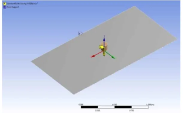
This study is considering the plate to be fixed on all 4 sides and a cylindrical body hits it with impact speeds from 1 to 20m/s. Also, the standard earth gravity is considered to be active.
The studies were carried out in ANSYS 12.1. Both, plate and body are considered to be made from structural steel.
At the impact, the geometry is presented in below figure:
Figure 1 The geometry at the impact
Also, in Figure 1are presented the boundary conditions and the axis of coordinate. X is the red vector, Y is the green vector and Z is the blue vector.
The origin is situated in the middle of the plate, at the intersection of the median surfaces.
The two bodies were meshed as below:
Figure 2 The meshed structure
The mesh of the plate consists in 4200 nodes and 1980 elements.
The simulations were a dynamic one, having the end time of 0.3 seconds.
For this paperwork were considered the normal stress (X axis).
The time variation of minimum and maximum values of normal stress (X axis) is presented in following pictures:
Figure 3 Time variation of minimum (red line) and maximum (green line) values of normal stress (X
250 DOI: 10.21279/1454-864X-16-I1-043
© 2015. This work is licensed under the Creative Commons Attribution-Noncommercial-Share Alike 4.0 License.
Figure 4 Time variation of minimum (red line) and maximum (green line) values of normal stress (X
axis) for 2m/s impact speed
Figure 5 Time variation of minimum (red line) and maximum (green line) values of normal stress (X
axis) for 3m/s impact speed
Figure 6 Time variation of minimum (red line) and maximum (green line) values of normal stress (X
axis) for 4m/s impact speed
Figure 7 Time variation of minimum (red line) and maximum (green line) values of normal stress (X
axis) for 5m/s impact speed
Figure 8 Time variation of minimum (red line) and maximum (green line) values of normal stress (X
axis) for 6m/s impact speed
Figure 9 Time variation of minimum (red line) and maximum (green line) values of normal stress (X
axis) for 7m/s impact speed
Figure 10 Time variation of minimum (red line) and maximum (green line) values of normal stress
(X axis) for 8m/s impact speed
Figure 11 Time variation of minimum (red line) and maximum (green line) values of normal stress
251 DOI: 10.21279/1454-864X-16-I1-043
© 2015. This work is licensed under the Creative Commons Attribution-Noncommercial-Share Alike 4.0 License.
Figure 12 Time variation of minimum (red line) and maximum (green line) values of normal stress
(X axis) for 10m/s impact speed
Figure 13 Time variation of minimum (red line) and maximum (green line) values of normal stress
(X axis) for 11m/s impact speed
Figure 14 Time variation of minimum (red line) and maximum (green line) values of normal stress
(X axis) for 12m/s impact speed
Figure 15 Time variation of minimum (red line) and maximum (green line) values of normal stress
(X axis) for 13m/s impact speed
Figure 16 Time variation of minimum (red line) and maximum (green line) values of normal stress
(X axis) for 14m/s impact speed
Figure 17 Time variation of minimum (red line) and maximum (green line) values of normal stress
(X axis) for 15m/s impact speed
Figure 18 Time variation of minimum (red line) and maximum (green line) values of normal stress
(X axis) for 16m/s impact speed
Figure 19 Time variation of minimum (red line) and maximum (green line) values of normal stress
252 DOI: 10.21279/1454-864X-16-I1-043
© 2015. This work is licensed under the Creative Commons Attribution-Noncommercial-Share Alike 4.0 License.
Figure 20 Time variation of minimum (red line) and maximum (green line) values of normal stress
(X axis) for 18m/s impact speed
Figure 21 Time variation of minimum (red line) and maximum (green line) values of normal stress
(X axis) for 19m/s impact speed
Figure 22 Time variation of minimum (red line) and maximum (green line) values of normal stress
(X axis) for 20m/s impact speed
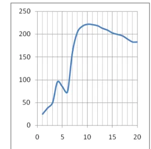
The maximum values for the normal stress (X Axis) for each impact speed, are presented below:
Table 1 Maximum values for the normal stress (X Axis) for different impact speed Sp ee d [m/ s] Normal stress (X Axis) [N/mm2]
Spee d [m/s]
Normal stress (X Axis) [N/mm2]
1 24.31 11 220.95
2 38.07 12 218.18
3 50.301 13 213.07
4 95.246 14 209.12
5 84.513 15 203
6 73.063 16 199.38
7 160.96 17 196.35
N o rm a l s tr e s s ( X Ax is ) [ N /m m 2] Speed [m/s]
Figure 23 Variation of the maximum values for Normal stress (X Axis) depending on impact
speed
It can be seen, at the impact speed of 8m/s it is reached a maximum value, and after that the values stays around this value.
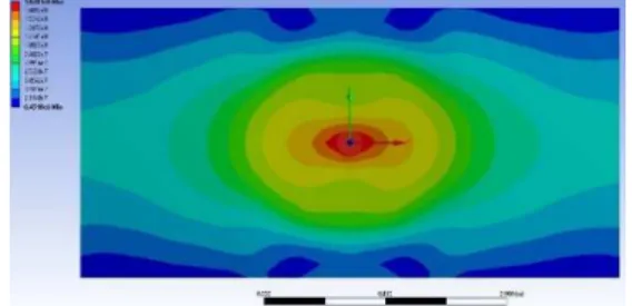
To understand the phenomenon we need to check the distribution diagrams for Normal stress (X axis) which are presented below:
Figure 24Distribution diagram for Normal stress (X Axis) when the maximum value is reached, for
253 DOI: 10.21279/1454-864X-16-I1-043
© 2015. This work is licensed under the Creative Commons Attribution-Noncommercial-Share Alike 4.0 License.
Figure 25 Distribution diagram for Normal stress (X Axis) when the maximum value is reached, for
2m/s impact speed
Figure 26 Distribution diagram for Normal stress (X Axis) when the maximum value is reached, for
3m/s impact speed
Figure 27 Distribution diagram for Normal stress (X Axis) when the maximum value is reached, for
4m/s impact speed
Figure 28 Distribution diagram for Normal stress (X Axis) when the maximum value is reached, for
5m/s impact speed
Figure 29 Distribution diagram for Normal stress (X Axis) when the maximum value is reached, for
6m/s impact speed
Figure 30 Distribution diagram for Normal stress (X Axis) when the maximum value is reached, for
7m/s impact speed
Figure 31 Distribution diagram for Normal stress (X Axis) when the maximum value is reached, for
8m/s impact speed
Figure 32 Distribution diagram for Normal stress (X Axis) when the maximum value is reached, for
254 DOI: 10.21279/1454-864X-16-I1-043
© 2015. This work is licensed under the Creative Commons Attribution-Noncommercial-Share Alike 4.0 License.
Figure 33 Distribution diagram for Normal stress (X Axis) when the maximum value is reached, for
10m/s impact speed
Figure 34 Distribution diagram for Normal stress (X Axis) when the maximum value is reached, for
11m/s impact speed
Figure 35 Distribution diagram for Normal stress (X Axis) when the maximum value is reached, for
12m/s impact speed
Figure 36 Distribution diagram for Normal stress (X Axis) when the maximum value is reached, for
13m/s impact speed
Figure 37 Distribution diagram for Normal stress (X Axis) when the maximum value is reached, for
14m/s impact speed
Figure 38 Distribution diagram for Normal stress (X Axis) when the maximum value is reached, for
15m/s impact speed
Figure 39 Distribution diagram for Normal stress (X Axis) when the maximum value is reached, for
16m/s impact speed
Figure 40 Distribution diagram for Normal stress (X Axis) when the maximum value is reached, for
17m/s impact speed
Figure 41 Distribution diagram for Normal stress (X Axis) when the maximum value is reached, for
255 DOI: 10.21279/1454-864X-16-I1-043
© 2015. This work is licensed under the Creative Commons Attribution-Noncommercial-Share Alike 4.0 License.
Figure 42 Distribution diagram for Normal stress (X Axis) when the maximum value is reached, for
19m/s impact speed
Figure 43 Distribution diagram for Normal stress (X Axis) when the maximum value is reached, for
20m/s impact speed
CONCLUSIONS
As it can be seen, the surface were the maximum values are distributed is increasing with the impact speed. This means the impact energy is distributed on bigger surface, and that’s why the maximum values of the normal stress (X axis) are topped around a value.
BIBLIOGRAPHY
[1] Ansys Workbench User Manual
[2] Huei – Huang Lee, Finite Element Simulations with Ansys Workbench 12, Schroff Development Corporation, ISBN 978-1-58503-604-2, 2010,
[3] Moaveni Saeed, Finite Element Analysis: Theory and applications with Ansys, 3rd edition,
ISBN978-0-13-189080-0, 2008
[4] O.C. Zienkiewicz, R.L. Taylor, The Finite Element Method for Solid and Structural Mechanics, 6th Edition,