www.the-cryosphere.net/8/1757/2014/ doi:10.5194/tc-8-1757-2014
© Author(s) 2014. CC Attribution 3.0 License.
Brief Communication: Trends in sea ice extent north of Svalbard
and its impact on cold air outbreaks as observed in spring 2013
A. Tetzlaff1, C. Lüpkes1, G. Birnbaum1, J. Hartmann1, T. Nygård2, and T. Vihma2,3
1Climate Sciences, Alfred-Wegener-Institut Helmholtz-Zentrum für Polar- und Meeresforschung, Bremerhaven, Germany 2Meteorological Research, Finnish Meteorological Institute, Helsinki, Finland
3Arctic Geophysics, The University Centre in Svalbard, Longyearbyen, Norway
Correspondence to:A. Tetzlaff ([email protected])
Received: 4 May 2014 – Published in The Cryosphere Discuss.: 6 June 2014
Revised: 4 August 2014 – Accepted: 20 August 2014 – Published: 25 September 2014
Abstract.An analysis of Special Sensor Microwave/Imager (SSM/I) satellite data reveals that the Whaler’s Bay polynya north of Svalbard was considerably larger in the three winters from 2012 to 2014 compared to the previous 20 years. This increased polynya size leads to strong atmospheric convec-tion during cold air outbreaks in a region north of Svalbard that was typically ice-covered in the last decades. The change in ice cover can strongly influence local temperature con-ditions. Dropsonde measurements from March 2013 show that the unusual ice conditions generate extreme convective boundary layer heights that are larger than the regional val-ues reported in previous studies.
1 Introduction
Arctic sea ice extent has strongly decreased in the last decade (Stroeve et al., 2012; Meier et al., 2012). This is most pro-nounced in summer and early autumn, during the period of sea ice melt, but there is increasing evidence for a nega-tive trend also during the remaining seasons (Stroeve et al., 2012). Cavalieri and Parkinson (2012) show that in March, sea ice extent declined by about 3 % decade−1from 1979 to 2010, but with large regional differences. For the Barents Sea and Greenland Sea regions, they find decline rates exceeding 5 % decade−1in winter and spring.
The latter regions are of special interest for ocean– atmosphere interactions due to frequent cold air outbreaks (CAOs) (e.g., Kolstad and Bracegirdle, 2008; Brümmer and Pohlmann, 2000; Chechin et al., 2013; Gryschka et al., 2008) with extremely large energy fluxes between ocean and
at-mosphere downstream of the ice margin. This means that, even if the number of CAOs remained unchanged, a po-sition change of the ice edge would have a strong impact on the local temperature conditions. This especially holds for the Svalbard archipelago, which is close to the Fram Strait marginal sea ice zone. It has been shown by Ivanov et al. (2012), Falk-Petersen et al. (2014), and Onarheim et al. (2014) that sea ice retreat is visible at the northern boundary of Svalbard by an increase of the “Whaler’s Bay polynya” extent (Fig. 1a). This sensible heat polynya forms due to the West Spitsbergen Current that causes upwelling of warm At-lantic water (Aagaard et al., 1987; Ivanov et al., 2012). Based on remote sensing data, Ivanov et al. (2012) observed a de-crease in the ice concentration north of Svalbard in winter and spring by more than 10 % in the period between 1999 and 2011 compared to the period between 1979 and 1995. Using a similar method, Onarheim et al. (2014) found an ice reduction of 10 % decade−1north of Svalbard between 1979 and 2012. They identify a temperature increase of the in-flowing Atlantic water as a major driver for this long-term trend, while the year-to-year variability is also influenced by wind direction. Both studies also found an increase in the near-surface air temperatures in the European Centre for Medium-Range Weather Forecasts (ECMWF) Re-Analysis Interim (ERA-Interim) data in this area, which is in line with the decreasing ice concentration in the last decades.
JFM
−10 °
0°
10°
20° 30° 40
° 50 ° 76°
78° 80°
82° 84°
1996
2012
P3 P2 P1 (a)
1992 1996 2000 2004 2008 2012
60 70 80 90 100
Year
Ice concentration (%)
(b)
Nov−May, Ivanov et al. 2012 Jan−Mar
1 30 60 90
1992 1996 2000 2004 2008 2012
Day of year (c)
Polynya length (km)
0 100 200 300 400 500 600 700
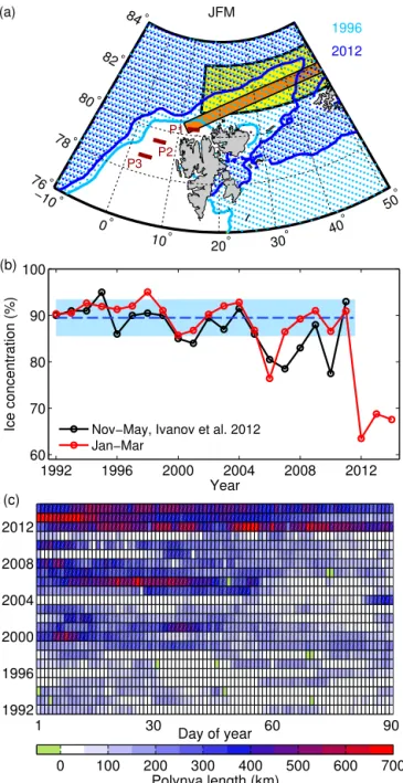
Figure 1.Mean JFM ice edge (based on 70 % SSM/I-ASI ice con-centration) in 1996 (light blue) and 2012 (dark blue), and areas used for calculation of the mean ice concentration in the Western Nansen Basin (WNB, yellow) and the length of the Whaler’s Bay polynya
(orange)(a). The three positions (P1–P3) used for the temperature
analysis are marked in dark red. Time series of the winter mean sea ice concentration in the WNB (red) with the 20-year mean and one
standard deviation (blue)(b). Data from Ivanov et al. (2012) are
shown for comparison (black). Polynya length for the years 1992
to 2014 as a function of day of the year(c). Green color denotes
missing data.
CAOs north of Svalbard. We present case studies of two CAOs in March 2013 that are influenced by the increased polynya extent. In addition, we use reanalysis data to
ana-lyze the impact of an increased polynya size on local tem-perature conditions. The evolution of the polynya extent is presented in Sect. 2, followed by the case studies in Sect. 3 and an analysis of the impact of the polynya size on atmo-spheric temperatures in Sect. 4.
2 Polynya size from 1992 to 2014
The wintertime (JFM) variability of the Whaler’s Bay sea ice cover between 1992 and 2014 is studied using daily Special Sensor Microwave/Imager (SSM/I) ice concentration data provided by Ifremer/CERSAT (http://cersat.ifremer.fr) with a spatial resolution of 12.5 km on the basis of the ASI re-trieval algorithm by Spreen et al. (2008).
We calculate the JFM mean ice concentration as in Ivanov et al. (2012) in a region northeast of Svalbard expanding from 15 to 60◦E and 81 to 83◦N referred to in the following as the
Western Nansen Basin (WNB). Although Ivanov et al. (2012) considered the period from November to May and used ice concentration data with 25 km resolution, the two time series of mean ice concentrations show the same general character-istics (see Fig. 1b). We find a 20-year mean of 89.5±4.0 %
from 1992 to 2011, which compares reasonably well with the value of 87.5±5.0 % by Ivanov et al. (2012) for this period.
In the winters of 2012 to 2014, however, there is a sudden decrease of the mean ice concentration to below 70 %, which is more than 4 standard deviations below the 20-year mean.
Another useful quantity is the polynya length, which is an important factor influencing the evolution of a convective at-mospheric boundary layer (ABL) during CAOs. We define the polynya length as the cumulative open-water path along the yellow area in Fig. 1a, starting at the northwestern edge of Svalbard. Here, we consider pixels with ice concentrations below 70 % as open-water areas. The polynya length is then the distance to the ice edge, that is, the first pixel exceeding 70 % ice concentration. Daily values of the polynya length are shown in Fig. 1c. In the winters of 1992 to 1998 the polynya length hardly ever exceeded 200 km, while lengths exceeding 300 km occurred more frequently between 1999 and 2011. As for mean ice concentration, 2012 to 2014 were also exceptional in terms of the polynya length, with values exceeding 400 km more than 40 % of the time. 2014 is also a remarkable year because the polynya length decreased from more than 500 km at the end of January to nearly 0 km in mid-April. The polynya remained closed at least until the be-ginning of August (status on 4 August 2014, not shown).
3 Cold air outbreaks north of Svalbard in March 2013
40 °
30° 20°
10°
10 m/s 84°
0° 82°
80°
78°
−10°
4 March 2013 (b)
Figure 2.Ice edge based on a 70 % threshold value of the
SSM/I-ASI ice concentration during days with cold air outbreaks:(a)26
March and(b)4 March 2013. The arrows denote the vertically
av-eraged wind in the boundary layer at the positions of the dropson-des. The lines are HYSPLIT backward trajectories at 10 m height
and the dots mark 10 h. Background of(a): MODIS visible image
at 12:45 UTC (http://lance-modis.eosdis.nasa.gov/cgi-bin/imagery/ realtime.cgi).
cloud streets over the Whaler’s Bay polynya clearly visible in satellite images (Fig. 2a). It was possible to document the strong convective regime, which is unusual for the region north of Svalbard (e.g., Brümmer and Pohlmann, 2000), by dropsondes released along flight tracks roughly parallel to the convection rolls. A detailed description of the dropsonde unit can be found in Lampert et al. (2012). In the following, we discuss two cases of CAOs causing convection over the polynya area on the basis of the dropsonde measurements.
On 4 March 2013 a CAO, developed west of Svalbard over the Fram Strait. It was caused by a strong high pressure sys-tem over Greenland and a low pressure channel expanding over the Barents and Kara Seas. Vertical profiles of wind, temperature, and humidity were obtained from six dropson-des released along 5◦E at distances of 0.5◦latitude (Fig. 2b).
250 260 270
0 0.5 1 1.5 2 2.5 3
−64 km
−5 km 48 km
104 km 161 km 214 km
Potential Temperature (K)
Height (km)
4 March 2013
(a)
250 255 260 265
−59 km 35 km 107 km
166 km 223 km
277 km 324 km 381 km
26 March 2013
(b)
0 200 400
0 0.5 1 1.5 2 2.5
Fetch (km)
Boundary layer height (km)
(c)
ARKTIS ’93 4 March 26 March
0 100 200 300 400 500
−25 −20 −15 −10 −5 0 5
ERA 2m temperature (
°
C)
Mean polynya length (km) (d)
2012 2013
2006 2014
P1 P2 P3
Figure 3.Potential temperature profiles from aircraft (black) and dropsonde (colored) data as a function of distance from the ice edge
on(a)4 March and(b)26 March 2013. The dots are aircraft
mea-surements at the dropsonde release points. Boundary layer height for those 2 days as a function of open-water fetch and data from
ARKTIS’93 (Brümmer, 1997) for comparison (gray)(c). JFM mean
ERA-Interim 2 m air temperature at three positions (P1–P3) north and west of Svalbard (see text) during times with wind from NE as
a function of polynya length from 1992 to 2014 (symbols)(d). The
We found the typical vertical temperature structure of a con-vective case with a well-mixed layer between the surface and a strong capping inversion together with an increasing temperature and atmospheric boundary layer height with dis-tance from the ice edge. This documents the convective char-acter of the ABL as found earlier during Fram Strait CAOs (Brümmer, 1997; Hartmann et al., 1997; Chechin et al., 2013; Lüpkes and Schlünzen, 1996; Wacker et al., 2005). The ver-tically averaged ABL potential temperature increased from 243 K at 64 km north of the ice edge by 18 K at 214 km south of it (Fig. 3a). Simultaneously, the boundary layer height increased from 150 m to about 2500 m, which is extremely large for this northern position.
The ABL height in CAOs depends on wind speed and temperature conditions. Another possible reason for the ex-treme ABL height at this latitude can be found by consider-ing the open-water fetch. A rough estimate of the open-water fetch can be derived from backward trajectories calculated for a height of 10 m using the HYSPLIT (HYbrid Single-Particle Lagrangian Integrated Trajectory) model transport and dispersion model by NOAA (Draxler and Rolph, 2013, see Fig. 2b). For the southernmost dropsonde, the fetch of 350 km was much larger than just the north–south distance to the ice edge of only 214 km. In this case the fetch is strongly increased due to northeasterly winds in contrast to the most frequent north–south orientation of CAOs. The large fetch might explain the extreme ABL height that is larger than any value published in the literature for this re-gion. The most comprehensive data set is from Brümmer (1997), who measured boundary layer growth during CAOs in the Fram Strait during the aircraft campaign ARKTIS’93 in March 1993. In that year, the ice edge was located at 80◦N
and the Whaler’s Bay polynya was nearly closed. Comparing our measurements to the ARKTIS’93 results (Fig. 3c), we find that the boundary layer height of 2500 m on 4 March, lo-cated at 78.5◦N, was larger than in all observed cases during ARKTIS’93. The largest boundary layer height observed by Brümmer (1997) was only about 2100 m at 77.5◦N, which is 100 km further to the south.
During another CAO on 26 March 2013, we observed boundary layer heights exceeding 1000 m, north of 80◦N (Fig. 3b and c). While this value is in the usual range of convective ABL heights during CAOs, it is quite unusual for this northern latitude. In this case northeasterly winds prevailed over the Whaler’s Bay polynya. Eight dropsondes were released during a flight from the northeastern edge of the polynya towards the region west of Svalbard (Fig. 2a). Here, the mean boundary layer potential temperature in-creased from 248 K over the pack ice to 257 K at the north-western corner of the Svalbard archipelago (Fig. 3b). The boundary layer height increased from 200 to a maximum of more than 1100 m. West of Svalbard the boundary layer char-acteristics stayed nearly the same since the fetch did not in-crease any more due to a more northerly wind direction. It
is also visible in Fig. 2a that the backward trajectories agree very well with the observed roll orientation.
4 Polynya impact on atmospheric temperatures
It is also interesting to consider the impact of polynyas on local atmospheric temperatures (e.g., Raddatz et al., 2013; Ebner et al., 2011; Fiedler et al., 2010). Using ERA-Interim data, Onarheim et al. (2014) found an air temperature in-crease of 7 K in the Whaler’s Bay polynya between 1979 and 2012 associated with the observed decrease in sea ice cover. The close connection between the size of the Whaler’s Bay polynya and the local temperature in the polynya region can be seen in Fig. 3d. There, we show ERA-Interim (Dee et al., 2011) 2 m air temperatures that are available every 6 h to de-termine the impact of the polynya size on local temperature conditions. The temperature is considered at grid points lo-cated north of Svalbard (80.25◦N, 12–15◦E , P1, see Fig. 1a)
and for northeasterly winds (30–60◦) only, which are identi-fied from the 10 m wind field of ERA-Interim.
The relationship between the JFM mean temperatures dur-ing northeasterly winds and the mean polynya length of the considered cases is probably not linear since tempera-tures will roughly approach the water temperature for larger polynya lengths. Therefore, we calculate the Spearman rank correlation that can be used to test the strength of a nonlinear relationship. We find a strong correlation ofrs=0.76. This is
in line with the more general findings by Ivanov et al. (2012), who concluded that air temperature trends in the Western Nansen Basin based on ERA-Interim data are consistent with the observed ice loss. Thus, depending on the temperature of the inflowing air masses, near-surface temperatures north of Svalbard can be more than 20 K higher in years with a large polynya extent compared to years with a closed ice cover.
To estimate how far south air temperatures are influenced by the polynya size, we repeat the calculations for two ad-ditional points further downstream. They are located north-west of Svalbard at 79.5◦N, 4.5–7.5◦E (P2 in Fig. 1a) and at 78.75◦N, 2.25–5.25◦E (P3 in Fig. 1a). The results are also shown in Fig. 3d. The Spearman rank correlation gradually decreases tors=0.52 at P2 andrs=0.42 at P3. Thus, an
ef-fect is still visible more than 200 km downstream. At ERA-Interim grid points even further to the south, the air temper-atures are nearly in equilibrium with the water tempertemper-atures and no significant correlations can be found.
5 Conclusions
cold air outbreaks and can have a large impact on the lo-cal temperatures around Svalbard. Based on ERA-Interim data within the polynya, we found that increased near-surface temperatures in this region are strongly related to a larger polynya extent. In addition, we observed an increase of the potential temperature by 9 K over the open water compared to the pack ice region during a CAO on 26 March 2013 north of Svalbard.
The increased fetch due to the larger polynya extent re-sults in events with strong roll convection in a region with usually stable stratification. We find a large ABL height in a region where such values have never been observed be-fore. Average boundary layer heights north of Svalbard are mostly below 300 m in winter according to an ERA-40 cli-matology from 1957 to 2002 by Wetzel and Brümmer (2011, their Fig. 7). A large extent of the Whaler’s Bay polynya is a precondition, however, a precondition for boundary layer heights exceeding 1000 m north of 80◦N during CAOs. We
observed a maximum boundary layer height of 2500 m in the Fram Strait at 78.5◦N, which is a large value for this latitude compared to other studies of CAOs (Brümmer, 1997; Hart-mann et al., 1997). With predictions of further shrinking of the Arctic sea ice volume in the next decades (e.g., Overland and Wang, 2013), a large Whaler’s Bay polynya, as observed from 2012 to 2014, might be present more often in the future. Increased boundary layer heights could also lead to a thicker cloud layer with enhanced precipitation. However, the analysis of ERA-Interim results did not show a significant correlation (not shown). It would be interesting to examine polynya-related changes in snowfall and a possible impact on the surface mass balance of glaciers in northern Svalbard in the future.
Acknowledgements. This work was partly funded by DFG (grant LU 818/3-1) and the Academy of Finland (grant 259537). We would like to thank M. Maturilli, who was in charge of the dropsonde unit. We also appreciate the helpful comments of the reviewers D. G. Barber and B. Brümmer.
Edited by: J. Stroeve
References
Aagaard, K., Foldvik, A., and Hillman, S. R.: The West Spitsbergen Current: disposition and water mass transformation, J. Geophys. Res., 92, 3778–3784, doi:10.1029/JC092iC04p03778, 1987. Brümmer, B.: Boundary layer mass, water, and heat
bud-gets in wintertime cold-air outbreaks from the Arctic sea ice, Mon. Weather Rev., 125, 1824–1837, doi:10.1175/1520-0493(1997)125<1824:BLMWAH>2.0.CO;2, 1997.
Brümmer, B. and Pohlmann, S.: Wintertime roll and cell convec-tion over Greenland and Barents Sea regions: a climatology, J. Geophys. Res., 105, 15559–15566, doi:10.1029/1999JD900841, 2000.
Cavalieri, D. J. and Parkinson, C. L.: Arctic sea ice variability and trends, 1979–2010, The Cryosphere, 6, 881–889, doi:10.5194/tc-6-881-2012, 2012.
Chechin, D. G., Lüpkes, C., Repina, I. A., and Gryanik, V. M.: Ide-alized dry quasi 2-D mesoscale simulations of cold-air outbreaks over the marginal sea ice zone with fine and coarse resolution, J. Geophys. Res., 118, 8787–8813, doi:10.1002/jgrd.50679, 2013. Dee, D. P., Uppala, S. M., Simmons, A. J., Berrisford, P.,
Poli, P., Kobayashi, S., Andrae, U., Balmaseda, A., Balsamo, G., Bauer, P., Bechtold, P., Beljaars, A. C. M., van de Berg, L., Bidlot, J., Bormann, N., Delsol, C., Dragani, R., Fuentes, M., Geer, A. J., Haimberger, L., Healy, S. B., Hersbach, H., Holm, E. V., Isaksen, L., Kallberg, P., Köhler, M., Matricardi, M., McNally, A. P., Monge-Sanz, B. M., Morcrette, J., Park, B., Peubey, C., de Rosnay, P., Tavolate, C., Thepaut, J., and Vitart, F.: The ERA-Interim reanalysis: configuration and performance of the data-assimilation system, Q. J. Roy. Meteor. Soc., 137, 553– 597, doi:10.1002/qj.828, 2011.
Draxler, R. and Rolph, G.: HYSPLIT (HYbrid Single-Particle Lagrangian Integrated Trajectory) Model access via NOAA ARL READY Website, available at: http://www.arl.noaa.gov/ HYSPLIT.php, last access: 5 June 2014, NOAA Air Resources Laboratory, College Park, MD, 2013.
Ebner, L., Schröder, D., and Heinemann, G.: Impact of Laptev Sea flaw polynyas on the atmospheric boundary layer and ice produc-tion using idealized mesoscale simulaproduc-tions, Pol. Res., 30, 7210, doi:10.3402/polar.v30i0.7210, 2011.
Falk-Petersen, S., Pavlov, V., Berge, J., Cottier, F., Kovacs, K. M., and Lydersen, C.: At the rainbow’s end: high productivity fu-eled by winter upwelling along an Arctic shelf, Polar Biol., 1–7, doi:10.1007/s00300-014-1482-1, 2014.
Fiedler, E. K., Lachlan-Cope, T. A., Renfrew, I. A., and King, J. C.: Convective heat transfer over thin ice covered coastal polynyas, J. Geophys. Res., 115, C10051, doi:10.1029/2009JC005797, 2010. Gryschka, M., Drüe, C., Etling, D., and Raasch, S.: On the influence of sea-ice inhomogeneities onto roll convec-tion in cold-air outbreaks, Geophys. Res. Lett., 35, L23804, doi:10.1029/2008GL035845, 2008.
Hartmann, J., Kottmeier, C., and Raasch, S.: Roll vortices and boundary-layer development during a cold air outbreak, Bound.-Lay. Meteorol., 84, 45–65, doi:10.1023/A:1000392931768, 1997.
Ivanov, V. V., Alexeev, V. A., Repina, I., Koldunov, N. V., and Smirnov, A.: Tracing Atlantic Water signature in the Arc-tic sea ice cover east of Svalbard, Adv. Met., 2012, 201818, doi:10.1155/2012/201818, 2012.
Kolstad, E. W. and Bracegirdle, T. J.: Marine cold-air outbreaks in the future: an assessment of IPCC AR4 model results for the Northern Hemisphere, Clim. Dynam., 30, 871–885, doi:10.1007/s00382-007-0331-0, 2008.
Lampert, A., Maturilli, M., Ritter, C., Hoffmann, A., Stock, M., Herber, A., Birnbaum, G., Neuber, R., Dethloff, K., Orgis, T., Stone, R., Brauner, R., Kässbohrer, J., Haas, C., Makshtas, A., Sokolov, V., and Liu, P.: The spring-time boundary layer in the Central Arctic observed during PAMARCMiP 2009, Atmo-sphere, 3, 320–351, doi:10.3390/atmos3030320, 2012.
Bound.-Lay. Meteorol., 79, 107–130, doi:10.1007/BF00120077, 1996.
Meier, W. N., Stroeve, J., Barrett, A., and Fetterer, F.: A simple approach to providing a more consistent arctic sea ice extent time series from the 1950s to present, The Cryosphere, 6, 1359–1368, doi:10.5194/tc-6-1359-2012, 2012.
Onarheim, I., Smedsrud, L., Ingvaldsen, R., and Nilsen, F.: Loss of sea ice during winter north of svalbard, Tellus A, 66, 23933, doi:10.3402/tellusa.v66.23933, 2014.
Overland, J. E. and Wang, M.: When will the summer Arctic be nearly sea ice free?, Geophys. Res. Lett., 40, 2097–2101, doi:10.1002/grl.50316, 2013.
Raddatz, R. L., Galley, R. J., Candlish, L. M., Asplin, M. G. and Barber, D. G.: Integral Profile Estimates of Sensible Heat Flux from an Unconsolidated Sea-Ice Surface, Atmos.-Ocean, 51, 135–144, doi:10.1080/07055900.2012.759900, 2013.
Spreen, G., Kaleschke, L., and Heygster, G.: Sea ice remote sens-ing ussens-ing AMSR-E 89-GHz channels, J. Geophys. Res., 113, C02S03, doi:10.1029/2005JC003384, 2008.
Stroeve, J., Kattsov, V., Barrett, A., Serreze, M., Pavlova, T., Hol-land, M., and Meier, W. N.: Trends in Arctic sea ice extent from CMIP5, CMIP3 and observations, Geophys. Res. Lett., 39, L16502, doi:10.1029/2012GL052676, 2012.
Wacker, U., Potty, K. V. J., Lüpkes, C., Hartmann, J., and Raschen-dorfer, M.: A case study on a Polar cold air outbreak over Fram Strait using a mesoscale weather prediction model, Bound.-Lay. Meteorol., 117, 301–336, doi:10.1007/s10546-005-2189-1, 2005.