www.nonlin-processes-geophys.net/13/177/2006/ © Author(s) 2006. This work is licensed
under a Creative Commons License.
in Geophysics
Multivariate autoregressive modelling of sea level time series from
TOPEX/Poseidon satellite altimetry
S. M. Barbosa, M. E. Silva, and M. J. Fernandes
Department of Applied Mathematics, Faculty of Science, University of Porto, Portugal
Received: 16 January 2006 – Revised: 30 March 2006 – Accepted: 18 April 2006 – Published: 20 June 2006
Abstract.This work addresses the autoregressive modelling of sea level time series from TOPEX/Poseidon satellite al-timetry mission. Datasets from remote sensing applications are typically very large and correlated both in time and space. Multivariate analysis methods are useful tools to summarise and extract information from such large space-time datasets. Multivariate autoregressive analysis is a generalisation of Principal Oscillation Pattern (POP) analysis, widely used in the geosciences for the extraction of dynamical modes by eigen-decomposition of a first order autoregressive model fit-ted to the multivariate dataset of observations. The extension of the POP methodology to autoregressions of higher order, although increasing the difficulties in estimation, allows one to model a larger class of complex systems. Here, sea level variability in the North Atlantic is modelled by a third or-der multivariate autoregressive model estimated by stepwise least squares. Eigen-decomposition of the fitted model yields physically-interpretable seasonal modes. The leading autore-gressive mode is an annual oscillation and exhibits a very ho-mogeneous spatial structure in terms of amplitude reflecting the large scale coherent behaviour of the annual pattern in the Northern hemisphere. The phase structure reflects the seesaw pattern between the western and eastern regions in the trop-ical North Atlantic associated with the trade winds regime. The second mode is close to a semi-annual oscillation. Mul-tivariate autoregressive models provide a useful framework for the description of time-varying fields while enclosing a predictive potential.
1 Introduction
Geophysical systems often exhibit complex variability pat-terns over a wide range of spatial and temporal scales. Obser-vation of the Earth by remote sensing techniques is yielding huge space-time datasets of geophysical observations. It is a challenging task to summarise and extract information from Correspondence to:S. M. Barbosa
such large datasets and characterise the dynamical properties of the associated geophysical time series.
This work focuses on the autoregressive modelling of time series of sea surface heights from TOPEX/Poseidon satel-lite altimetry mission. Sea level is a key indicator of climate change and an important observational constraint on global climate models. Furthermore, sea level changes have consid-erable environmental, social and economical impacts. The height of the sea surface relative to a geocentric reference ellipsoid is measured from space through radar altimetry. TOPEX/Poseidon (T/P) mission achieved an unprecedented accuracy, yielding a huge, high quality, space-time dataset of precise sea level measurements.
A stochastic space-time process{Xs,t}is defined as a
col-lection of random variables indexed by parameters[s, t]∈R2
where t indicates time and s a location. Observed values of {Xs,t}from mspatial locations (s=1, ..., m) at N times
(t=1, ..., N) constitute a realisation of the stochastic process {Xs,t}. The term field is used hereafter to designate a
partic-ular realisation and is denoted by
Xt = [X1,tX2,t...Xm,t]T ∈Rm×1, t =1, ..., N. (1)
Statistical space-time methods play a key role in the analy-sis of time-varying fields. Given an observed fieldXt,
di-mensionality reduction, spatio-temporal description and ex-traction of dominant variability modes are often primary goals. In the case of systems dominated by nonlinear inter-actions, nonlinear methods for dimensionality reduction are required, such as the Isomap procedure (Tenenbaum et al., 2000; G´amez et al., 2004), based on the replacement of Eu-clidean by geodesic distances, or nonlinear principal compo-nent analyses (Hsieh, 2001; Hsieh and Wu, 2002). Modelling of nonlinear systems requires methods extending the linear empirical models to a nonlinear setting such as in Kravtsov et al. (2005) and Kondrashov et al. (2005). However, lin-earity is assumed henceforth as a first approximation to the dynamics of the system.
analysis method for extraction of the dominant variabil-ity patterns from an observed field (Preisendorfer, 1988; Von Storch and Zwiers, 1999; Jollife, 2002). PCA yields dominant spatial structures, in terms of maximal variance ex-plained and the corresponding temporal evolution for these structures; the observed field is decomposed into modes of variability, each of which is the product of a spatial pat-tern and a time-varying amplitude. Although principal com-ponents (PCs) are often interpretable, dynamical modes are not necessarily uncorrelated and/or yielding maximal vari-ance. Furthermore, PCA depends on the size and shape of the spatial domain. Thus interpretation of PCs as physi-cal/dynamical modes must be always done with caution.
Principal Oscillation Pattern (POP) analysis (Hasselman, 1988; Von Storch et al., 1995; Von Storch and Zwiers, 1999) yields dynamical modes from a spatio-temporal dataset through the analysis of a stochastic model fitted to the ob-servations. POP analysis assumes that the observed field has a temporal autoregressive structure of order one, i.e. follows a m-variateAR(1)model
Xt =AXt−1+εt (2)
whereA∈Rm×m is the matrix of real autoregressive coeffi-cients andεt is a temporally uncorrelated noise vector with
mean0 and covariance matrix6∈Rm×m. A first order au-toregressive model is the discrete-equivalent of a first order ordinary differential equation and thus corresponds, depend-ing on the autoregressive parameters, to a combination of stochastically forced relaxators and oscillators. If a first or-der multivariate autoregressive model provides an adequate fit to the observed field, the dynamical characteristics of the system can be empirically inferred from the fitted model, as-suming the space-time characteristics of the model to be rep-resentative of the full system. The eigen-decomposition of the autoregressive model describing the temporal evolution of the field yields the dominant modes of variability from the multivariate dataset in terms of relaxation and oscillation modes. From eigen-decomposition of the matrix Aof au-toregressive coefficients,A=PLP−1, the state of the system at any timetcan be expressed as
Xt = m
X
k=1
uktpk (3)
where the eigenvectors pk (the columns of matrix P) are
the principal oscillation patterns (POP) or empirical normal modes, and the time seriesukt are the coefficient time se-ries, computed from the adjoint patternspak (eigenvectors of AT) as ukt=pakTXt. In the absence of noise the
eigenvec-tors of matrixAare the system normal modes, representing the natural modes of variability of the evolving field. Com-plex eigenvaluesλj=rjeiwj are associated under stationary
conditions (|λj|≤1, j=1, ..., m) to damped oscillations with
characteristic damping raterj and frequencywj while real
eigenvalues describe damped, non-oscillatory, patterns.
POP analysis yields a space-time description of dominant variability modes and can also be used for prediction, but the applicability of POP analysis is restricted to fields for which an AR(1) model provides an adequate fit to the ob-servations. However, the methodology can be generalised, allowing to model a larger class of systems, by extending the analysis to autoregressive models of arbitrary order p,
AR(p)(L¨utkepohl, 1993; Neumaier and Schneider, 2001). Multivariate autoregressive models (m−AR(p)), also called vector autoregressive models (VAR), are the most used mod-els for multiple time series and are being increasingly used in geophysical applications (e.g. Maharaj and Wheeler, 2005; Rashid and Simmonds, 2005).
In this study sea level variability in the North Atlantic is examined through multivariate autoregressive modelling. The paper is organised as follows. Multivariate autoregres-sive analysis is summarised in Sect. 2. The particular appli-cation of multivariate autoregressive modelling to the anal-ysis of sea level observations from satellite altimetry is de-scribed in Sect. 3. Concluding remarks are presented in Sect. 4.
2 Multivariate autoregressive analysis
2.1 Multivariate autoregressive modelling
Am−variate autoregressive model of orderp(m−AR(p)) is defined as
Xt =A1Xt−1+A2Xt−2+ · · ·ApXt−p+εt (4)
whereAi∈Rm×mi=1· · ·pare the matrices of autoregressive
coefficients and εt∈Rm is a temporally uncorrelated noise
vector with mean0and covariance matrix6∈Rm×m. The fit of a m−AR(p) model to a time-varying field involves the selection of the model order p and the es-timation of the model parameters A1,A2· · ·Ap, 6 from
a spatio-temporal dataset. The model order can be se-lected by minimising an order selection criterion such as the Schwartz Bayesian Criterion (SBC) (Schwarz, 1978) reflect-ing the trade-off between over-fittreflect-ing and over-simplification. The SBC is superior in terms of consistency to the Akaike Information Criterion (AIC) and the Final Prediction Er-ror Criterion (FPE) as discussed in L¨utkepohl (1993). A
m−AR(p) model can be cast in the form of a regression model and the parametersA1,A2· · ·Ap estimated by least
missing values, the least squares estimator for am−AR(p)
model is consistent and asymptotically normal (L¨utkepohl, 1993) and is recommended, provided that the model to be fit-ted is stable (Schneider and Griffies, 1999). Difficulties in the estimation of am−AR(p)are often associated with the large number of parameters involved. For large fields the number of spatial degrees of freedom can be reduced by consider-ing the leadconsider-ing components from a PCA analysis thereby re-ducing dimensionality while retaining most of the variance in the original field. Although PCA is a multivariate anal-ysis method for independent observations, and thus should not be used for time series, non-independence does not have a serious effect when the main objective of the analysis is descriptive rather than inferential (Jollife, 2002). A positive by-product of estimating a multivariate autoregressive model in PCA space is the exclusion of noisy components from the analysis and diagonalisation of the error covariance matrix. 2.2 Multivariate autoregressive modes
Am−AR(p)model can be written as a first order model
m−AR(1),
e
Xt =eAXet−1+eεt (5)
where Xet=[Xt,Xt−1· · ·Xt−p+1]T∈Rm×p, εet=[εt 0. . .0]T
with covariance matrix e6=
C 0 0 0
∈Rmp×mp and e
A∈Rmp×mp is the augmented covariance matrix given
by
e A=
A1A2 Ap
I 0 0
0 I
..
. . .. ...
0 0 0
. (6)
Since am−AR(p)model can be formulated as a first order autoregressive model, higher order multivariate autoregres-sive models can be used, analogously to POP analysis, to infer the dynamical characteristics of a system through de-composition into eigenmodes with characteristic oscillation periods and damping times.
Eigen-decomposition of the augmented coefficient matrix e
A as eA=ePLeP−1, where P=[pe
1pe2...epmp] is the matrix of
eigenvectors andL is the diagonal matrix of the eigenval-uesλk, k=1, ..., mp yields mpm-dimensional eigenmodes
(Neumaier and Schneider, 2001). Complex eigenvalues
λj=rjeiwj correspond to damped oscillatory modes with
periodTj=2π/wj and characteristic damping raterj or
e-folding time −1/ ln(rj) (the time interval in which a
ex-ponentially decaying quantity decreases to 1/eof its previ-ous value). Real eigenvalues correspond to damped, non-oscillatory modes.
3 Multivariate autoregressive analysis of sea level series
Multivariate autoregressive analysis is illustrated for the time series of sea level observations from TOPEX altimeter. 3.1 Data
The analysed altimetry data are measurements from TOPEX altimeter for the North Atlantic. The dataset covers nearly 12 years from September 1992 to March 2005 (cycles 1 to 460) at approximately 10-days intervals (9.9156 days, corre-sponding to the satellite repeat period). Corrected sea sur-face heights are derived from the Merged Geophysical Data Records (MGDR) products (AVISO, 1996) by applying stan-dard instrumental and geophysical corrections and editing procedures, including the Inverse Barometer (IB) correction (Dorandeu and Le Traon, 1999), the smoothing of TOPEX dual frequency ionospheric correction (Fernandes and An-tunes, 2003), the cycle dependent drift effect in the wet tro-pospheric correction derived from the onboard TOPEX Mi-crowave Radiometer (Scharroo et al., 2004), the sea state bias (SSB) correction (Chambers et al., 2003) and a residual SSB correction of−3 mm applied to cycles 236 and greater (Berwin, 2003). Tides are removed using the NAO99b model (Matsumoto et al., 2000). Sea level anomalies are derived by subtracting to corrected sea surface heights the GSFC00.1 mean sea surface model (Wang, 2001).
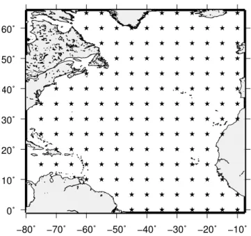
For each cycle, a regular 5 degree grid of altimetry data is obtained from the along-track measurements. In order to avoid spatial aliasing and eliminate redundant data spatial blocks with size equal to the grid spacing are considered and the along-track observations within every non-empty block are replaced by a median position and value. Regular grids of sea level anomalies are then obtained using the adjustable tension continuous curvature surface gridding algorithm of Smith and Wessel (1990), with a tension value of 0.35, which is the value suggested by experience for topography data. The resulting dataset comprises 153 time series of sea level anomalies at the grid nodes (Fig. 1) at approximately 10-days intervals (m=153 locations,N=460 observations). The typ-ical standard deviation for the time series of sea level anoma-lies is below 5 cm.
3.2 Multivariate autoregressive modelling
−80˚ −70˚ −60˚ −50˚ −40˚ −30˚ −20˚ −10˚ 0˚
10˚ 20˚ 30˚ 40˚ 50˚ 60˚
Fig. 1.Study area (North Atlantic) and time series locations (*).
Neumaier and Schneider (2001) and the code of Schneider and Neumaier (2001). The mAr package has been released under GPL (General Public License) Version 2 and is avail-able from the CRAN repository (http://www.cran.r-project. org).
3.2.1 Data preprocessing
Altimeter records are short and include substantial high-frequency variability associated with mesoscale circulation. Denoising based on the discrete wavelet transform is an ef-ficient way to remove high frequency variability from the satellite altimetry time series while preserving non-smooth features (Barbosa et al., 2005). Variability at scales shorter than 20 days is reduced through nonlinear thresholding in the wavelet domain using the universal level-dependent thresh-old rule (Donoho and Johnstone, 1995) yielding an overall reduction in variability of sea level anomalies of 1 cm.
The gridded dataset of denoised sea level anomalies is standardised by subtracting the mean and dividing each time series by its standard deviation. The normalisation of the sea level series allows one to obtain spatial patterns with-out possible domination by gridpoints with larger variances. Although avoiding the problem of spatial variability being driven by the most energetic gridpoints, normalisation yields coefficients corresponding to standardised sea level, which are therefore less easy to interpret directly.
PCA is carried out on the normalised field for dimension-ality reduction. The large number of spatial degrees of free-dom is reduced by considering a truncated PCA version of the original sea level field. A subspace ofk=8 principal
com-0 10 30 50 70 90 110 130 150
70
80
90
100
PC number
% variance explained
Fig. 2.Fraction of variance accounted by the principal components (PC).
2 4 6 8 10
−4.0
−3.5
−3.0
p
SBC
Fig. 3.Schwartz Bayesian Criterion (SBC) as a function of model order (p).
ponents (PCs) is considered, explaining more than 85% of the overall variance of the sea level field (Fig. 2).
3.2.2 Model estimation
A multivariate autoregressive model is estimated for the de-noised and normalised sea level field. The estimation of the parameters in the model is carried out in the PCA subspace by least squares. The Schwartz Bayesian Criterion (SBC) is used for selection of the orderpof the model (Fig. 3). The plot shows that a considerable improvement in model fit (as measured by SBC) is obtained by considering rather than a first order (corresponding to the assumption in POP analysis) higher order models. The SBC criterion suggests a model of orderp=3.
Table 1. Statistics of model fit for each variable: residual sum of squares (RSS), R-square, F statistic and corresponding p-value.
Variable RSS R-square F p-value
PC1 08.55 0.9998 93 093 <10−16
PC2 02.72 0.9995 39 440 <10−16
PC3 11.58 0.9972 6397 <10−16
PC4 14.28 0.9939 2949 <10−16
PC5 06.59 0.9955 4015 <10−16
PC6 07.81 0.9930 2553 <10−16
PC7 12.40 0.9884 1541 <10−16
PC8 04.87 0.9947 3403 <10−16
Table 2. Eigenmodes for the sea level field estimated from the
m−AR(3)model.
Period (years) e-folding time (years)
0.97 9.70
0.52 0.94
However such agreement can be misleading due to the dan-ger of overfitting in which case the model is not a parsimo-nious representation of the multivariate dataset. A trade-off between parsimony and agreement with observations is un-avoidable and to a large extent dependent on the objectives of the analysis. If the model is used for forecasting for example, a “worst” fit may yield better predictions; on the other hand if the model is used to describe and understand the measured system a closer agreement between the model and the dataset may be preferable.
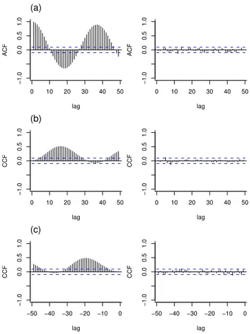
Since a multivariate autoregressive process can be in-terpreted as a filter that transforms the observations into white noise series, uncorrelatedness of the residuals is a pri-mary criterion for checking the adequacy of an estimated model. The autocorrelation function for the leading compo-nent (Fig. 4a) indicates that the model yields a uncorrelated residual series. Figures 4b and c show that the estimated model is able to describe the relationship between the first two leading components of the observed field yielding un-correlated residual series. These results suggest that the fitted model is an adequate representation of the sea level field. 3.2.3 Eigenmodes
Eigenmodes are computed from the eigen-decomposition of the coefficients matrix from them−AR(3)model. The esti-mated model is stable since for all the eigenvalues|λi|<1∀i.
Only sustained modes, as measured by the corresponding e-folding time (e-e-folding>period), are considered (Table 2).
0 10 20 30 40 50
−1.0
0.0
0.5
1.0
lag
ACF
(a)
0 10 20 30 40 50
−1.0
0.0
0.5
1.0
lag
ACF
0 10 20 30 40 50
−1.0
0.0
0.5
1.0
lag
CCF
(b)
0 10 20 30 40 50
−1.0
0.0
0.5
1.0
lag
CCF
−50 −40 −30 −20 −10 0
−1.0
0.0
0.5
1.0
lag
CCF
(c)
−50 −40 −30 −20 −10 0
−1.0
0.0
0.5
1.0
lag
CCF
Fig. 4.Correlation of leadings PCs (left) and corresponding
resid-uals from the estimatedm−AR(3)model (right): (a)
autocorre-lation, PC1;(b)cross-correlation, PC1 & PC2 (positive lags);(c)
cross-correlation, PC1 & PC2 (negative lags). Horizontal dashed lines represent 95% confidence levels for correlation of white noise realisations. Lags are spaced by 10 days.
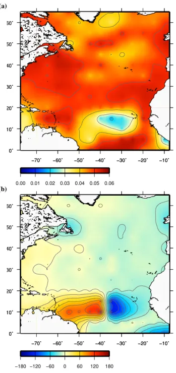
The leading, least damped mode, associated with the largest eigenvalue, is an annual oscillation. The second mode is close to a semi-annual oscillation. These are natural modes, since the seasonal signal is usually the dominant sig-nal in sea level time series. The structure of the autoregres-sive modes is represented by the amplitude (A) and phase (ψ) obtained from the real (pr)and imaginary (pi) components of the associated eigenvectorsp=pr+ipi as A=
q p2
r+pi2
andψ=arctan(pi/pr).
(a)
0˚ 10˚ 20˚ 30˚ 40˚ 50˚ 60˚
−70˚ −60˚ −50˚ −40˚ −30˚ −20˚ −10˚
0˚ 10˚ 20˚ 30˚ 40˚ 50˚ 60˚
−70˚ −60˚ −50˚ −40˚ −30˚ −20˚ −10˚
0.00 0.01 0.02 0.03 0.04 0.05 0.06 (b)
0˚ 10˚ 20˚ 30˚ 40˚ 50˚ 60˚
−70˚ −60˚ −50˚ −40˚ −30˚ −20˚ −10˚
0˚ 10˚ 20˚ 30˚ 40˚ 50˚ 60˚
−70˚ −60˚ −50˚ −40˚ −30˚ −20˚ −10˚
−180 −120 −60 0 60 120 180
Fig. 5.First autoregressive mode:(a)Amplitude;(b)Phase.
throughout the North Atlantic except for the seesaw in the tropical Atlantic, reflecting opposing phases on the west and east sides. Sea level in this region is closely related with the winds regime. The relaxation of trade winds at the beginning of the year (February–March) causes a decrease in sea level on the west side and an increase on the east side; the onset of trade winds in May–June is responsible for a decrease in the sea level in the east and an increase in the west (Schouten et al., 2005). A difference in phase is also visible along the coast of Newfoundland and Ireland.
(a)
0˚ 10˚ 20˚ 30˚ 40˚ 50˚ 60˚
−70˚ −60˚ −50˚ −40˚ −30˚ −20˚ −10˚
0˚ 10˚ 20˚ 30˚ 40˚ 50˚ 60˚
−70˚ −60˚ −50˚ −40˚ −30˚ −20˚ −10˚
0.00 0.04 0.08 0.12 0.16 0.22
(b)
0˚ 10˚ 20˚ 30˚ 40˚ 50˚ 60˚
−70˚ −60˚ −50˚ −40˚ −30˚ −20˚ −10˚
0˚ 10˚ 20˚ 30˚ 40˚ 50˚ 60˚
−70˚ −60˚ −50˚ −40˚ −30˚ −20˚ −10˚
−180 −120 −60 0 60 120 180
Fig. 6.Second autoregressive mode:(a)Amplitude;(b)Phase.
4 Conclusions
Remote sensing of the Earth is yielding large datasets of geo-physical observations in both time and space. Finding pat-terns from an observed field is a challenging task, even more challenging when one comes to interpretation. The use of au-toregressive models as linear approximations to the dynamics of a field has a strong physical motivation, since autoregres-sions can be interpreted as discretised verautoregres-sions of ordinary differential equations.
Multivariate autoregressive models constitute an useful ex-tension to POP analysis. By considering higher order mod-els, a larger class of systems can be modelled. Multivari-ate autoregressive models allow the extraction of dominant modes of variability from an observed field. Similarly to POP analysis, if a multivariate autoregressive model of arbi-trary orderpprovides an adequate fit to the observations of an observed field, the dynamical characteristics of the field can be empirically inferred from the fitted model through eigen-decomposition, yielding the dominant modes of vari-ability from the multivariate dataset in terms of relaxations and oscillations. A drawback of the approach is the large number of parameters that need to be estimated, leading to difficulties in estimation and stability. Estimation is thus car-ried out in reduced PCA space for dimensionality reduction. When fitting an autoregression to an observed field, the es-timation method and the number of principal components to retain when considering the field in PCA reduced space are important issues that must be handled on an application-specific basis.
Here satellite altimetry observations in the North Atlantic have been modelled by a multivariate autoregression of third order. The estimated model is according to SBC a signif-icantly better representation of the observed sea level field than a first order model. Eigendecomposition of the fitted autoregressive model yielded physical interpretable modes, constituting a useful space-time description of North Atlantic sea level variability. Although only seasonal modes have been inferred by autoregressive modelling, this is a limita-tion of the dataset (strongly constrained by the short length of the satellite altimetry series) rather than of the approach itself.
Autoregressive models have a predictive potential. Thus the estimation of a multivariate autoregressive model can be applied not only to produce a space-time description in terms of dominant variability modes, as in this work, but also to prediction. Although the linear stationary nature of autoregressive models implies the decay of the oscillatory solutions, which is an undesirable property in a forecasting framework, this can be handled by assuming a constant uni-tary amplitude for prediction from an estimated model. In the sea level application discussed here, forecasting is ham-pered by the short length of the available time series. With the expected increasing length of sea level series as satellite
missions extend in time, forecasting sea level from an autore-gressive model should become feasible.
Acknowledgements. This work has been supported by program POCTI through the Centro de Investigao em Ciencias Geo-espaciais (CICGE) of the Faculty of Science, University of Porto.
Edited by: M. Thiel
Reviewed by: H. Rust and three other referees
References
AVISO: AVISO User Handbook for Merged TOPEX/POSEIDON Products, AVI-NT-02-101-CN ed. 3.0, 1996.
Barbosa, S. M., Fernandes, M. J., and Silva, M. E.: Space-time analysis of sea level in the North Atlantic from TOPEX/Poseidon satellite altimetry, International Association of Geodesy Sym-posia, 129, 248–253, Springer, 2005.
Berwin, R.: Topex/Poseidon Sea Surface Height Anomaly Product. User’s Reference Manual, NASA JPL Physical Oceanography DAAC, Pasadena, CA., 2003.
Chambers, D. P., Hayes, S. A., Ries, J. C., and Urban, T. J.: New Topex sea state bias models and their effect on global mean sea level, J. Geophys. Res., 108, 3305–3311, 2003.
Donoho, D. L. and Johnstone, I. M.: Adapting to unknown smooth-ness via wavelet shrinkage, J. Amer. Stat. Assoc., 90, 1200–1224, 1995.
Dorandeu, J. and Le Traon, P. Y.: Effects of global mean at-mospheric pressure variations on mean sea level changes from TOPEX/Poseidon, J. Atmos. Oceanic Technol., 16, 1279–1283, 1999.
Fernandes, M. J. and Antunes, M. A.: Eight years of radar altime-try in the North-East Atlantic, Proceedings 3 Assembleia Luso-Espanhola de Geodesia e Geofisica, 1, 226–230, 2003.
G´amez, A. J. G., Zhou, C. S., Timmermann, A., and
Kurths, J.: Nonlinear dimensionality reduction in climate
data, Nonlin. Processes Geophys., 11, 393–398, 2004,
http://www.nonlin-processes-geophys.net/11/393/2004/. Hasselman, K.: PIPs and POPs: The reduction of complex
dynam-ical systems using principal interaction and oscillation patterns, J. Geophys. Res., 93, 11 015–11 021, 1988.
Hsieh, W. W.: Nonlinear principal component analysis by neural networks, Tellus A, 53, 599–615, 2001.
Hsieh, W. W. and Wu, A.: Nonlinear multichannel
singu-lar spectrum analysis of the tropical Pacific climate variabil-ity using a neural network approach, J. Geophys. Res., 107, doi:10.1029/2001JC000957, 2002.
Jollife, I. T.: Principal Component Analysis, Springer, 2002. Kondrashov, D., Kravtsov, S., Robertson, A. W., and Ghil, M.: A
hi-erarchy of data-based ENSO models, J. Climate, 18, 4425–4444, 2005.
Kravtsov, S., Kondrashov, D., and Ghil, M.: Multi-level regression modeling of nonlinear processes: derivation and applications to climatic variability, J. Climate, 18, 4404–4424, 2005.
L¨utkepohl, H.: Introduction to Multiple Time Series Analysis, Springer, 1993.
Matsumoto, K., Takanezawa, T., and Masatsugu, O.: Ocean tide models developed by assimilating Topex/Poseidon altimeter data into hydrodynamical model: a global model and a regional model around Japan., J. Oceanography, 56, 567–581, 2000.
Neumaier, A. and Schneider, T.: Estimation of parameters and eigenmodes of multivariate autoregressive models, ACM – Transactions on mathematical software, 27, 27–57, 2001. Preisendorfer, R. W.: Principal Component Analysis in Meteorolgy
and Oceanography, Elsevier, 1988.
R Development Core Team: R: A language and environment for statistical computing, R Foundation for Statistical Computing, Vienna, Austria, http://www.R-project.org, ISBN 3-900051-07-0, 2005.
Rashid, H. A. and Simmonds, I.: Southern Hemisphere annular mode variability and the role of optimal nonmodal growth, J. At-mos. Sci., 62, 1947–1961, 2005.
Scharroo, R., Lillibridge, J. L., Smith, W. H. F., and Schrama, E. J. O.: Cross-calibration and long term monitoring of the mi-crowave radiometers of ERS, TOPEX, GFO, Jason and Envisat, Marine Geodesy, 27, 279–297, 2004.
Schneider, T. and Griffies, S. M.: A conceptual framework for pre-dictability studies, J. Climate, 12, 3133–3155, 1999.
Schneider, T. and Neumaier, A.: ARfit – A MATLAB package for the estimation of parameters and eigenmodes of multivariate au-toregressive models, ACM Transactions on Mathematical Soft-ware, 27, 58–65, 2001.
Schouten, M. W., Matano, R. P., and Strub, T. P.: A description of the seasonal cycle of the equatorial Atlantic from altimeter data, Deep Sea Res. I, 52, 477–493, 2005.
Schwarz, G.: Estimating the dimension of a model, Annals of Statistics, 6, 461–464, 1978.
Smith, W. H. F. and Wessel, P.: Gridding with continuous curvature splines in tension, Geophysics, 55, 293–305, 1990.
Tenenbaum, J. B., de Silva, V., and Langford, J. C.: A global ge-ometric framework for nonlinear dimensionality reduction, Sci-ence, 290, 2319–2323, 2000.
Von Storch, H. and Zwiers, F. W.: Statistical Analysis in Climate Research, Cambridge University Press, 1999.
Von Storch, H., Burger, G., Schnur, R., and von Stoch, J.: Principal Oscillation Patterns: a Review, J. Climate, 8, 377–399, 1995. Wang, Y. M.: Mean Sea Surface, gravity anomaly, and vertical