Nonlinear Processes
in Geophysics
c
European Geosciences Union 2002
On the problem of optimal approximation of the four-wave kinetic
integral
V. G. Polnikov1, *and L. Farina1
1Centro de Previs˜ao de Tempo e Estudos Clim´aticos (CPTEC), Instituto Nacional de Pesquisas Espaciais (INPE), CPTEC/INPE, Cachoeira Paulista, SP, 12630-000, Brazil
*permanent address: The State Oceanographic Institute, Moscow, Russia Received: 19 March 2002 – Revised: 2 July 2002 – Accepted: 25 July 2002
Abstract.The problem of optimization of analytical and nu-merical approximations of Hasselmann’s nonlinear kinetic integral is discussed in general form. Considering the gen-eral expression for the kinetic integral, a principle to obtain the optimal approximation is formulated. From this con-sideration it follows that the most well-accepted approxi-mations, such as Discrete Interaction Approximation (DIA) (Hasselmann et al., 1985), Reduced Integration Approxima-tion (RIA) (Lin and Perry, 1999), and the Diffusion Approxi-mation proposed recently in Zakharov and Pushkarev (1999) (ZPA), have the same roots. The only difference among them is, essentially, the choice of the 4-wave configuration for the interacting waves. To evaluate a quality of any approxima-tion for the 2-D nonlinear energy transfer, a mathematical measure of relative error is constructed and the meaning of approximation efficiency is postulated. By the use of these features it is shown that DIA has better accuracy and effi-ciency than ZPA. Following to the general idea of optimal approximation and by using the measures introduced, more efficient and faster versions of DIA are proposed.
1 Introduction
It is well known (Komen et al., 1994) that a suitable descrip-tion of a wind-generated ocean wave field is given by the two-dimensional wave energy spectrum distribution through the space and in time, S(σ, θ,x, t ). Here (σ, θ )is the an-gular frequency and the angle of propagation of the individ-ual wave component, respectively; x = (x, y) is the geo-graphical space coordinate vector andtis the time of evolu-tion. In the theory, an evolution equation for waves is usu-ally written in the form of a transport equation for the so-called wave action spectrum distribution in the wave vector k-space,N (k,x, t ). In deep water and in absence of ambient Correspondence to:V. G. Polnikov
([email protected] or [email protected])
currents it has the form
∂N ∂t +
vg(k)∂N ∂x
=FN,k,U, (x, t )≡I N+N L−DI SS. (1) In Eq. (1),vg(k)is the group velocity of the wave compo-nent with wave vector k, F (...)is the source function de-scribing the balance of energy for waves under consideration andU(x, t) is the local wind. Usually, the source function includes the energy-input term, I N, the quasi-conservative nonlinear wave-wave interaction term,N L, and the wave en-ergy dissipation term,DI SS (Komen et al., 1994). Corre-spondence between wave action spectrum,N(k), and energy spectrum,S(σ, θ ), is given by the relationship
N (k)dk= 4π 2g
σ S(σ, θ )dσ dθ. (2)
In general, the wave vectorkis related to the frequencyσby the dispersion relation
σ2=gktanh[kD(x)] (3)
where D(x)is the local depth, andk is the module of the vectork. Later in this paper we shall restrict ourselves by consideration of the deep-water case when Eq. (3) reduces to
σ2=gk.
In the following, the main attention will be placed on the
N L-term. In several papers it was shown that theN L-term plays a principal role in ocean wave evolution (see, for ex-ample, Young and van Vledder, 1993; Komen et al., 1994). For this reason and due to a great mathematical difficulty in-volved in its study, research on this topic is ongoing for the last forty years, since the pioneering paper by Hasselmann (1962).
is governed by the kinetic integral
N L= ∂N (k4)
∂t ≡TN(k)=4π Z
dk1 Z
dk2 Z
dk3M2
(k1,k2,k3,k4)×hN (k1)N (k2) N (k3)+N (k4)
−N (k3)N (k4) N (k1)+N (k2)i
δ σ (k1)+σ (k2)
−σ (k3)−σ (k4)δ(k1+k2−k3−k4) (4) Here (ki = 1, 2, 3, 4) are the wave vectors of interacting waves,σ1 = σ (ki)are the corresponding angular frequen-cies of the wave due to dispersion relation,TN(k)is the non-linear transfer of wave action, and M (...) are the matrix elements describing an intensity of interaction of four waves. The delta-functions in Eq. (4) assure that the four interacting waves should meet the following resonance conditions k1+k2=k3+k4, (5)
σ1+σ2=σ3+σ4. (6)
A joint solution of Eqs. (5) and (6) defines a special reso-nance 3D surface in the 8-dimensionalk-space. In a discrete representation, this surface give rises to a set of 4-wave con-figurations for wave vectorski contributing to the real non-linear transfer of wave energy among waves.
Due to symmetry properties of the matrix elementsM, the nonlinear transfer formally conserves the total wave energy
E=
Z
N (k)σ dk, (7)
total wave action
A=
Z
N (k)dk, (8)
and total wave moment M=
Z
N (k)kdk. (9)
All these features of the kinetic integral result in specific properties of the real nonlinear transferTN(k). The prop-erties of theN L-term in a ocean wave model are dictated by the properties of the kinetic integral (4).
The problem of describing theN L-term can be divided into two aspects:
1. A theoretical study of the kinetic integral properties; 2. The implementation of the theoretical results into a
practice of wind wave numerical modeling.
The explicit analytical expression of the integrand in Eq. (4) is rather complicated (see, for example, Hasselmann, 1962, or, in more convenient form, Crawford et al., 1980). In addition to this, the multifold integration in Eq. (4) is to be carried out on a specific 3D-surface in the 8-dimensional k-space with a singular locus. For these reasons a theoretical study of the kinetic integral properties is a very difficult task in the wind wave theory. This task gave rise to strong efforts
of numerous investigators, aimed to find the real properties of the nonlinear energy transfer among surface gravity waves (Zakharov and Filonenko, 1966; Webb, 1978; Masuda, 1980; Hasselmann et al., 1981, 1985; Polnikov, 1989, 1990, 1994, 2001; Resio and Perry, 1991)1. Up to present, this part of the wind wave theory is practically solved (possibly excluding some details of long term nonlinear evolution (Lavrenov and Polnikov, 2001), and the main interest is addressed to imple-mentation of the theory into practical numerical modeling.
Nowadays it is evident that the exact calculation of the ki-netic integral can not be directly introduced into operational ocean wave models due to the large consuming time for this calculation. Therefore, one should use some kind of approx-imation to the exact integral. This is an important problem in the practice of wind wave numerical modeling, which, in turn, has theoretical and practical aspects. This paper is just devoted to consideration of the former. The latter will be considered in a separate paper.
The outline of the paper is the following. In Sect. 2 several present approximations of the two- dimensionalN L-term are discussed, and main unsolved tasks are posed. Section 3 is devoted to a general consideration of the problem. From this consideration it follows that the most advanced approxima-tions have the same mathematical root. A problem of ap-proximation efficiency and optimization of apap-proximation is posed and solved. In Sect. 4 a mathematical measure is intro-duced to estimate a relative error of any approximation with respect to exact 2-D nonlinear energy transfer among waves. The theory derived is used on the example of two alternative approximations in Sect. 5. In Sect. 6 two new versions of DIA are proposed, and their greater accuracy and efficiency are shown. Section 7 contains the final conclusions.
2 Statement of the problem
First of all, we should mention that there are several pro-posals dealing with numerical and analytical approximations for the kinetic integral. They have been presented both for one- dimensional (1-D) nonlinear transfer (Barnett, 1968; Resio, 1981; Zakharov and Smilga, 1981) and for the two-dimensional (2-D) one (Hasselmann et al, 1981; Hasselmann et al., 1985, Polnikov, 1991; Zakharov and Puchkarev, 1999, Lin and Perry, 1999; Hashimoto and Kawagushi, 2001; Van Vledder, 2001; and so on). For additional bibliography one may be referred to books: SWAM group (1985), Efimov and Polnikov (1991), Komen et al. (1994). In this paper we shall mainly focus on the approximations of the 2-D nonlinear transfer, which are more relevant for the modern wind wave modeling.
Among numerous 2-D approximations, one can select only a few that are theoretically well substantiated. The main feature of such an approximation should be its direct math-ematical relation to the original kinetic integral. Actually, these approximations are as follow.
1. Diffusion approximation (DA) which was for the first time proposed in Hasselmann et al. (1981) and later elaborated in Zakharov and Pushkarev (1999) and Jenk-ins and Phillips (2001);
2. Discrete Interaction Approximation (DIA) proposed in Hasselmann et al. (1985) and elaborated in Hashimoto and Kawagushi (2001), Van Vledder (2001);
3. Reduced Integration Approximation (RIA) proposed in Lin and Perry (1999).
The dates of references mentioned permit us to hope that we consider the state-of-the art situation.
Here we shall try to analyze the main points of these ap-proximations with the aim to find a way for an optimal so-lution of the problem. As far as a diffusion approximation proposed by Hasselmann (1981) is not practically used, we start our analysis from the more widely used Discrete Inter-action Approximation.
2.1 Discrete interaction approximation
The main idea of DIA is to take into account only one certain configuration of the four interacting waves. To do this, Has-selmann et al. (1985) have proposed to use the configuration, which in the polar coordinates(σ, θ )has the form:
(1)k1=k2=k,where the arbitrary wave vectork is represented byσandθ;
(2)k3=k+, wherek+is represented byσ+=σ (1+λ)
andθ+=θ+1θ+; (10a)
(3)k4=k−, where is represented byσ−=σ (1−λ) andθ−=θ−1θ−;
(4)In consistency with the conditions(5)and(6),parameters of the configuration are
λ=0.25, 1θ+=11.5◦,and1θ−=33.6◦. (10b)
In such an approach, in accordance with Eq. (4), the nonlin-ear transfer at all mentioned k-points takes the form
∂N (k−) ∂t
=I (k,k+,k−),∂N (k+)
∂t =I (k,k+,k−), ∂N (k)
∂t = −2I (k,k+,k−), (11)
where
I (k,k+,k−)=Cg−8σ19
N2(k)(N (k+)+N (k−))−2N (k)N (k+)N (k−)
(12)
D(1σ,˜ 1θ ).˜
In Eq. (12) the fitting constant isC =3000, andD(1σ,˜ 1θ )˜
is the differential expressed in non-dimensional increments of the integration grid, 1σ,˜ 1θ˜ , (for the fixed grid,D is a constant). The net nonlinear transfer at any fixed(σ, θ )-point is found by the procedure of running of Eqs. (11) through all points of the frequency-angle integration grid{σi, θj}.
The main advantage of this approximation is its evident simplicity and rather good efficiency for certain initial spec-tra (Hasselmann et al., 1985). For this reason, it is widely used in practical wave modeling. The so-called WAM model (Komen et al., 1994) is an example of a successful implemen-tation of DIA. One of the technical shortages of DIA routine used in WAM is the presence of intermediate and cumber-some interpolation operations provided by the mismatch of spectral grid nodes and the vectorsk+,k−. This leads to a large increase in the integration time.
In some papers (Polnikov, 1991; Zakharov and Pushkarev, 1999; Van Vledder, 2000; Lin and Perry, 1999; Jenkins and Phillips, 2001) it was mentioned that the accuracy of DIA is not reasonable for the JONSWAP spectrum. This stimulated some authors to a search for a more efficient approximation of the nonlinear term (see, for example, papers mentioned above and Hashimoto and Kawagushi, 2001; Van Vledder, 2001). Authors of the two latter papers tried to modify DIA by introduction of new and multiple configurations. How-ever, it seems that these efforts did not significantly change the situation. Thus, the problem of DIA improvement is not achieved yet.
2.2 Diffusion approximation
For the first time the diffusion approximation (DA) was pro-posed in Hasselmann et al. (1981) by considering the exact integral (4) in the small scattering angle approximation. But the final expression for DA in this paper is rather compli-cated. A more elegant form of DA was proposed in Zakharov and Pushkarev (1999) and Jenkins and Phillips (2001) re-cently. Their results are not based on the explicit expres-sion for the exact kinetic integral; they used the conservation laws (7)–(9) and inspection of some particular analytical so-lutions. Nevertheless, as it was shown in Polnikov (2002), that both of these proposals can be derived directly from the exact kinetic integral, if one estimates the final result for in-tegral (4) as the contribution of the most contributive config-uration
k1∼=k2∼=k3∼=k4. (13) The use of this configuration is the main idea of the diffu-sion approximation. We note here that sometimes this idea is mentioned as the hypotheses of locality for nonlinear inter-actions.
Detailed analysis of the DA is given in Polnikov (2002). For this reason we will not elaborate here on this point but restrict ourselves to the following remarks.
and Phillips (2001) is the same as the one by Zakharov and Pushkarev (1999). Moreover, both of them are based on the same theoretical considerations. Thus, a consideration of the latter is sufficient for our aims below. Thirdly, following Pol-nikov (2002), the approximation by Zakharov and Pushkarev (1999) is considered as the most promising alternative to the DIA due to its relative mathematical simplicity and effective-ness.
So, the diffusion approximation due to Zakharov and Pushkarev (1999) (ZPA) has the following form
∂N (k)
∂t =
c′ σ3L
n3(k)σ24, (14)
where Lis the linear differential operator of the following form
L= 1
2
∂2 ∂σ2+
1
σ2 ∂2
∂θ2 (15)
andc′ is the fitting constant of the order of 0.05 (Polnikov, 2002)2.
It is important to note that according to Polnikov (2002), a preliminary (very qualitative) estimation of the relative ac-curacy of ZPA is of the order of 50%. Herewith, a rigorous mathematical definition of accuracy was not introduced in Polnikov (2002), and the real accuracy of ZPA (and DIA as well) is now known. Thus, we should state that the point of estimation of accuracy for theN L-term approximation is unsolved yet.
2.3 Reduced integration approximation
Another kind of approximation was proposed in Lin and Perry (1999), which was called as the Reduced Integration Approximation (RIA). To derive the latter, Lin and Perry (1999) placed their most attention on the fact that the inte-grand in Eq. (4) is growing infinitely for some configurations whenk2 → k4 andk1 → k3 (the singularity of integrand mentioned earlier). It permitted them to reduce the threefold integral (4) to a quasi-linear one with a rather small interval of variations fork1andk3in the vicinity ofk4. By this man-ner they reduce the time of integration radically with con-serving a reasonable accuracy of the final result for the non-linear transfer. In our notations, RIA takes the form
∂n(k4) ∂t =4π
k4+1k Z
k4−1k dk3
θ4+1θ Z
θ4−1θ dθ3
M3(k3,k4,k3,k4)Jδ(k3,k4,k3,k4)N3(k3,k4), (16) where Jδ(k3,k4,k3,k4) is a rather complicated Jacobian due to integration of delta-functions in Eq. (4),N3(k3,k4) is the proper cubic form of wave spectra, and1k, 1θ, are the special fitting parameters of the approximation.
As one can see, the net expression of the reduced integral in RIA is more complicated when compared to DIA and DA. 2The optimal fitting constants both in DIA and DA are varying in dependence of the spectral shape.
In addition to this, RIA needs to use matrix elementsMfor calculations, which have to be calculated and stored previ-ously. All these restrictions reduce the efficiency of RIA. Comparison of configurations used in Eq. (16) and Eq. (13) shows that RIA can be considered as a mixed version of DIA and DA. It looks like some a kind of multiple DIA but for DA-configuration (13). Thus, the properties of RIA resem-ble ones for DA (see Lin and Perry, 1999).
Finally, we should mention here again that neither Lin and Perry (1999) nor others authors proposed a rigorous mathe-matical procedure for inter-comparison of different approx-imations for the exact kinetic integral. For this reason we have not ways to get a rigorous estimating the accuracy of any certain approximation.
All these uncertainties gave rise to the appearance of new approximations among which different modifications of DIA (Hashimoto and Kawagushi, 2001; Van Vledder, 2001) and DA (Zakharov and Pushkarev, 1999; Jenkins and Phillips, 2001; Polnikov, 2002) are looked like as the most promising. 2.4 Problems posed
Now we can formulate a set of tasks of the present paper, concerning unsolved theoretical points of the problem for optimization of the N L-term approximation. They are as follows. 1) To consider the problem in general form and to find the common and differing features of the approximations mentioned above. 2) To establish a rigorous measure of ef-ficiency of approximations for the exact kinetic integral. 3) To define a mathematical procedure for comparing accuracy and efficiency of different approximations. 4) To test DIA and ZPA with respect to their accuracy and efficiency. 5) To propose an approximation, which is more efficient than any other considered above. All these problems will be treated and solved in the present paper.
3 Phylosophy of the approach
3.1 General point of view
We start from simplifying a representation of the kinetic inte-gral. According to Polnikov (1989), after an exact analytical integration of the wave vector delta-function with respect to k2and the frequency delta-function with respect toθ1, in po-lar coordinates the integral (4) takes the form
∂N4 ∂t =c
X
±
Z Z Z
M12±,2±,3,4 J k2±
N1±N2±(N4+N3)−N4N3(N1±+N2±) (17)
dσ1dσ3dθ3,
wherecis the dimensional coefficient depending ong, Ni =
N (σi, θi),J is the Jacobian of the frequency delta-function integration,k2±is the modified wave number corresponding
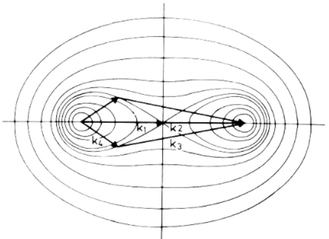
Fig. 1. Visual representation of the configurations permitted by Eqs. (5) and (6). Contour lines correspond to the possible end points of interacting vectors. Example is shown for the original DIA con-figuration given by Eq. (10) (Hasselmann et al., 1985).
form of J is not needed for understanding the after going text. We only note that the Jacobian detects a 3D singular surface, which defines the most contributive configurations of interacting waves.
From Eq. (17) one can see that in a discrete representa-tion of the integrarepresenta-tion grid{σig, θjg}, the integral (17) can be written as a simple sum of the form
∂N4 ∂t =c
X
i
Ri(N3)iDi = X
i
Bi N1±N2±(N4+N3)−N4N3(N1±+N2±)i, (18)
whereiis the number of allowed interacting configuration. In Eq. (18)Ri is the spectrum independent part of the inte-grand in Eq. (17),(N3)iis the cubic spectral form, andDiis the integration differential in the frequency-angle space (the sub-indeximeans that the values are taken for a proper teracting configuration). After grouping of all spectrum in-dependent parts of the summands,cRiDi ≡Bi, the final sum takes a simple form. Note thatBi is the fixed constant for a certain configuration of four vectorsk1,k2,k3,k4. In the (σ, θ )-spaceBi is proportional to the scaling factorσ19(see Eq. 12) and is depending on the angles between vectors of configuration only.3
Analysis of Eq. (18) allows us to find common and differ-ing features of various approximations mentioned in Sect. 2 and to generate ideas about optimal approximation for the integral Eq. (17).
As we mentioned above, configurations of four wave vec-torsk1,k2,k3,k4contributing to the integral should meet the resonant conditions Eq. (5) and Eq. (6). Herewith, the
3There is an additional (rather strong) dependence ofB i on its
location at the singular surface (see Polnikov, 1989), but it is less important from the configuration point of view.
most contributive configurations include the points at the singular surface. As was shown in Masuda (1980), Pol-nikov(1989), some of such configurations are corresponding to the condition
k1=k2=(k3+k4)/2=ka/2 (19) wherekais the reference vector of the configuration. Com-paring Eq. (19) with Eq. (10) one can see that this condition is the basis of DIA.
It is well known that a lot of other configurations are lo-cated at the singular surface. They can be represented by the “figure-of-eight” in the Longett-Higgins diagram (Fig. 1). The most contributive of them (for which the value ofRi is going to infinity with the greatest rate) corresponds to the configuration
k1=k2=k3=k4. (20) According to Eq. (13), this is just the configuration used in DA (and RIA).
Thus, from this consideration one can see that DIA, DA and RIA has the same root. All of them are based on the account for contribution of certain configurations at the sin-gular surface. In fact, original DIA and different variants of DA are based on a one configuration only. The multiple DIA (with its variations) or RIA has a number of configurations and does not essentially differ from DIA. Thus, the approxi-mations under consideration have a common origin.
The only technical difference between DA and DIA (RIA) is provided by the fact that the cubic spectral formN3 be-comes equal to zero for configuration (20). For this reason, one should take a Tailor’s expansion of the cubic form in the vicinity of the point (20), which leads to the diffusion op-erator representation of the DA, as was shown in Polnikov (2002).
From the analysis above, we can conclude:
1. The most adequate (theoretically grounded) approxima-tions employ the wave-number configuraapproxima-tions allocated at the singular surface of the integrand in Eq. (17). 2. The only difference between the approximations DIA,
DA, and RIA is the choice of set of the contributing configurations.
3. The optimal approximation for integral (17) can be de-fined as one leading to the highest efficiency of approx-imation. Such a kind approximation can be constructed by means of choosing a special set of the contributing configurations, if the definition of efficiency is given. 3.2 Efficiency of approximation
The term “efficiency of approximation” is often used in the literature mentioned above, but it was never formulated in exact mathematical form. Here we address this point.
the time of one-step calculation,τ.4 These two parameters should be used in the definition of efficiency of approxima-tion. Usually these two parameters are in a competitive con-text: one is working against the other. In general, it is not so simple to say which of them is more preferable. To do this, one needs some postulates depending on the specific goal. For this reason, it seems that the term “efficiency” is the more intuitive (or qualitative) parameter of the ap-proximation. Nevertheless, in this sub-section we introduce some postulates and formulate the meaning of the term “effi-ciency” in a mathematical form.5
Firstly, we state here that the accuracy (or relative error) of the numerical approximation of the integral (17) is more important than other aspects. Let us consider this point in more detail.
To calculate the relative error,εrel, of the approximation, one should have a reference value of the exact kinetic inte-gral. As far as the integral (17) in a closed form is not known, the so-called “exact calculation” is to be done numerically as well. This procedure has its own relative error with respect to the “exact theoretical value” of the kinetic integral (which corresponds to the theoretical definition of integration)6. The relative error of the “exact calculation” can be estimated by traditional means, i.e. by making the integration grid reso-lution to be finer and finer. Eventually, we can state that the “exact calculation” is executed by using a proper mathemati-cal algorithm and by using a certain frequency-angle grid for integration in Eq. (17).
Appropriate algorithms for this task are well known (se references above). How to choose the standard frequency-angle grid, and how should be the relative error of “the exact calculation”? To answer these questions, one should “a pri-ori” introduce the lower limit value of the relative error for the approximated calculation ofN L-term, εaplim. Taking in mind numerous ambiguities of the source term in Eq. (1), one may postulate that the lower limit of relative error of the approximation should be not smaller than 10–15%, i.e.
εlimap ∼=0.10−0.15. This means that for practical aims there is sufficient to have an approximation forN L-term the rela-tive error of which meets the following condition
εrel ≥εaplim∼=0.10−0.15. (21) On the other hand, it is reasonable to assume that the re-quested relative error of the “exact calculation”,εlimex , must be at least one order smaller:
εlimex ∼=0.1εaplim∼=0.01−0.015. (22) 4The mathematical definition of ε
rel will be given later in
Sect. 4. Relative accuracy,αrel, is related to the relative error,εrel,
by the evident simple ratio:αrel=1−εrel. In the after going text
both terms are used.
5Here we consider the efficiency for the one-step calculation of the kinetic integral. The point of the long-term efficiency is rather similar but more complicated due to the absence of the commonly recognized opinion about features of the long-term solution of the kinetic Eq. (4) (see discussion in Lavrenov and Polnikov, 2001).
6Note that in the aspect of accuracy, the time of “exact calcula-tion” does not play any role.
From this, one may conclude that for estimation of the relative error of the N L-term approximation, the value of
εexlim should be of the order of 1–2%. Thus, the standard frequency-angle grid may be of any kind which provides the necessaryεlimex . This is the first theoretical conclusion deal-ing with the accuracy consideration. As seen, it leads to the constraint (22) on the features of the standard integration grid needed for the estimation ofεrel.
Existence of different standard frequency-angle grids is known from numerous calculations (Hasselmann et al., 1981; Masuda, 1980; Polnikov, 1989; and so on). A certain ex-ample for one of them will be given later in the following section.
Consider now the issue of computation time. For practical purposes, one may separate the following two types of com-putation time for the N L-term calculation: (1) a “relative integrating time”, and (2) a “one-step time”. The fist type of time is defined by the relative part of the CPU- time, RP, taken by theN L-term sub-routine in numerical model calcu-lations as a whole. The second type of time is defined by the real CPU-time,τ, needed for the calculation ofN L-term at one step in time.
A definition of efficiency is different for different values ofRP. This fact results in to possibility of introduction the following two meanings: the first type efficiency,Eff1, and the second type efficiency,Eff2.
In the first case, whenRP ≪ 1, there is a natural upper limit for “the relative integrating time” of theN L-term cal-culation, based on the following practical consideration. If the time ofN L-term calculations takes less than 15–20% of the total time of prognostic calculations in a numerical model (RP ≤0.15−0.2), there is no need to reduceRPmore, as far as the other part of the model takes the major time of CPU. Therefore, in such a case, the first type efficiency may be defined by the relative error of N L-term approximation only. A heuristic formula for efficiency could be proposed in the following form
Eff1∝(εrel)−p. (23)
Here the powerpis introduced to emphasize the role of ac-curacy (or relative error) in the definition of approximation efficiency. As far as in the “error theory” just the second power of error plays a main role (for example, for summa-tion of errors), we may specify the power valuepto be equal to 2. Then, if we accept the highest limit of efficiency to be about 100 units, the best formula forEff1corresponding to the lower limit ofεrel(21) takes the form
Eff1=(εrel)−2 (24)
In the second case, when the relative part ofN L-term cal-culations is sufficiently large (for example, RP > 0.2), it is reasonable to suppose that the efficiency of approximation depends inversely on the one-step time ofN L-term calcula-tion, τ, to the power of RP. In accordance with Eq. (24)
Eff2can be given as
where Tref is the reference time introduced for normaliza-tion of the value of the timeτ. Here,Tref should be always smaller thanτ (see the definition ofTref below). The power
RP is introduced to emphasize the role of calculation time as an auxiliary parameter. It means that for rather small val-ues ofRP (whenRP becomes much less than 1 andτ is of the order ofTref), the second type efficiency,Eff2, should degenerate into the efficiency of the first type,Eff1.
To close the point, we need to specify the reference time
Tref. To do this, we accept the definition thatTref is the time taken by the calculation of N L-term in a “fast one-configuration approximation” given by Eqs. (11) and (12) without any intermediate interpolation procedures7. In such a case, the more configurations and more intermediate (inter-polation) procedures are involved into a certain approxima-tion, the greater a real one-step timeτ is for this approxima-tion. Consequently, the ratioTref/τ becomes smaller. As a result, the total efficiency is balanced by the relative error of the approximation according to Eq. (25).
Final conclusions of this sub-section are the following. 1. The term “efficiency” is rather an intuitive and
qualita-tive parameter of the approximation.
2. The efficiency of a numerical approximation of theN L -term depends on several parameters in the calculation process. They are: the relative error of approximation,
εrel; time of one-step integration,τ; relative part of time taken by N Lterm subroutine from the whole time of prognostic calculations,RP; and some heuristic mag-nitudes, such as the powerpin Eq. (23) and reference time of “the simple one-configuration approximation”,
Tref.
3. The role of accuracy is more important than the role of the computation time in the approximated calculation of theN L-term. It means that for approximations with equivalent efficiency, the one with more accuracy (or less errorεrel) is preferable.
4. The efficiency of approximation has its natural upper value (of the order of 100 conventional units) which is absolutely sufficient for practical goals.
3.3 Optimization of approximation
In accordance with the said above, the efficiency of any ap-proximation is balanced by two competitive characteristics: the accuracy and the computation time. By definition, the op-timal approximation corresponds to the best balance between relative error,εrel, and the one-step time of calculation,τ, which provides the highest efficiency. Thus, an optimal ap-proximation for integral (17) is provided by the choice of optimal set of the contributing configurations.
Here we should note that for any fixed set of configura-tions, the value of the relative error of approximation,εrel, depends on the shape of spectrum under the integral. For this
7A point of the spectrum interpolation is discussed in Sect. 6.
reason an estimation of the efficiency is not so simple as it seems from a first sight. We believe that the finding of the ef-ficiency of approximation is not a purely technical task but, rather, is some kind of an expertise process. To carry out this process, one needs to select an appropriate set of reference spectra. Such a kind of set will be proposed in Sect. 5 after getting a preliminary experience of efficiency estimating. In the course of these preliminary calculations a certain speci-fication will be done for the choice of the reference time of calculation,Tref.
4 Measure of relative error
We consider the following two-dimensional functions: (a) The exact nonlinear energy transfer in the frequency-angle space,Tex(σ, θ ), obtained by a certain numerical algorithm at the standard integrating grid for a certain spectral shape of the energy spectrumS(σ, θ )8; (b) The approximated nonlin-ear energy transferTap(σ, θ ), at the same space, obtained for the same energy spectrum and at the same frequency-angle grid by any numerical algorithm.
The problem to be addressed is how to estimate the non-dimensional relative error of the approximation,εrel rigor-ously and systematically. Regarding the 2-D nonlinear trans-fer, this problem was never discussed in the literature. There-fore, some of the following statements will be rather heuris-tic.
Some initial specifications are now opportune9.
1. The 2-D functions Tex(f, θ ) and Tap(f, θ ) are to be given at a properly chosen frequency-angle grid
(fig, θjg)(at the so-called “standard integrating grid” providing a necessary accuracy of Tex(f, θ ), see Sect. 3).
2. For simplifying the comparison of the results for dif-ferent spectral shapes, all values of Tex(f, θ ) and
Tap(f, θ )are to be normalized by a certain dimensional coefficient depending on the peak frequency, fp, and the peak value of the 2-D spectrum,Sp. In our calcu-lations the nonlinear transfer functions are calculated in conventional units of the normalizing coefficient, Cn, introduced in Polnikov (1989)
Cn=(π/16)g−4fp11S 3
p. (26)
3. Due to an ambiguity in the fitting coefficient for the ap-proximated transfer,Tap(f, θ )(see Sect. 2), one should adjust the latter toTex(f, θ )by an additional adjusting coefficient, Cad. In our work this coefficient is esti-mated by means of the least-square-root method in ac-8The meaning of the terms “exact” and “the standard integrating grid” were clarified earlier in Sect. 3.
cordance with the condition Z
Tex(f, θ )−Cad(ia)Tap(ia)(f, θ ) 2
df dθ=min.,(27)
where(ia)means the individual index of approxima-tion, andis the fixed part of the frequency-angle space used for estimation ofCad. In our calculations the do-main covers the whole frequency-angle grid under consideration. With some algebra, one can find the fol-lowing expression forCad:
Cad(ia)()=
R
Tex(f, θ )Tap(ia)(f, θ )df dθ
R
Tap(ia)(f, θ ) 2
df dθ
. (28)
4. Finally, the properly adjusted nonlinear transfer for the
(ia)-th approximation, used for the error estimation, has the following value
Tap(ia)(f, θ )=Tap, init(ia) (f, θ )∗Cad(ia), (29) where the domain factoris omitted for simplicity. Now one can introduce a formula for the relative error,
εrel. For this aim, a traditional measure can be used. For example,
εrel(ia)(ε)= R ε
Tex(f, θ )−Tap(ia)(f, θ ) 2
df dθ
R
Tap(ia)(f, θ ) 2 df dθ
1/2
(30)
whereεis the fixed part of the frequency-angle space used for estimation of εrel. However, the measure (30) is too smooth, as far as it is not sensitive to the location of the points where the nonlinear transfer changes the sign. Nevertheless, it seems reasonable that the proper measure must include in its definition this very important feature of theN L-transfer responsible for the spectrum shape evolution. For this reason we prefer the formula which is more sensitive to this feature of the nonlinear transfer function. After some analysis we made the option for the following measure ofεrel:
εrel(ia)(ε)= R ε
Tex(f, θ )−Tap(ia)(f, θ )
Tex(f, θ )
m df dθ R ε df dθ 1/m (31)
with the choice ofm=1. The more typical choice,m=2, was not acceptable because it gives the relative error mea-sure too sensitive to the zero-crossing feature of the nonlinear transfer.
We should note that the definition (31) could be easily transformed to the case of the 1-D N L-transfer, T (f ) =
H
T (f, θ )dθ. In fact, for the 1-D relative error, εrel,1−D, the transformation of Eq. (31) is
ε(ia)rel,1−D(ε)= R ε
Tex(f )−Tap(ia)(f )
Tex(f )
df R ε df (32)
In principle, the 1-D relative error is less interesting in our analysis. Nevertheless, in the present paper, it will be con-sidered in some cases, for generality.
Finally, we need to say some words about a choice of the domainε. In the general case, it is possible to analyze rel-ative errors for several types of domains. But later we shall mainly deal with results only for the 10%-threshold domain defined by the following ratio
ε=10%∈ |Tex(f, θ )| ≥0.1R, (33) where
R=T+−T−. (34)
HereT+is the positive extremum of the exact 2-D nonlin-ear transfer andT− is the negative one. Owing to the inte-gral feature of the relative error (31), hereafter it is called the mean relative error (MRE). For generality, the first estima-tions of errors will be presented for 20%-threshold domain as well. In the following section the proposed approach will be applied to estimation of the MRE and efficiency for two alternative approximations: DIA and ZPA, the most prospec-tive ones at present time.
5 Estimations of errors and efficiency for DIA and ZPA
5.1 Numerical specifications
For the calculation of the exact nonlinear energy transfer,
Tex(σ, θ ), we have used the algorithm proposed in Polnikov (1989) and the code by the same co-author. The code for DIA was extracted from the widely used version of WAM (Cycle 4) with minor programming adjustments to our task. The code for ZPA was written in accordance with Eqs. (14) and (15) (for details, see Polnikov, 2002).
The standard frequency-angle grid,(fi, θj), used for our calculations, is defined by the following ratios
f (i)=f0·ei−1, (35)
θ (j )= −π+j·(π/18), (36)
with the following values of the grid parameters: f0 = 0.7462,e=1.05, and 1≤i≤41,0≤j ≤35. The relative error of “the exact estimations” forTex(σ, θ )is about 1–3%. For more generality we have used the following two-mode spectrum representation
S(f, θ )=S1(f, θ, fp1, θp1, γ1, s1)
-80 -60 -40 -20 0 20 40 60 80
0,75 0,82 0,91 1,00 1,10 1,22 1,34 1,48 1,63 1,80 1,98 2,18 2,41 2,65 2,93 3,23 3,56 3,92 4,32 4,77 5,25
exact-nl-1
dia-nl-1
zakh-nl-1
Ts(f)
f
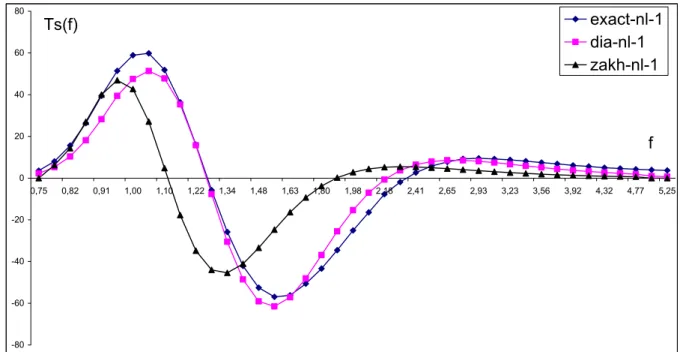
Fig. 2.Visual representation of 1-D-nonlinear transfer∂S(f )/∂t =Ts(f )for the exact calculation and adjusted DIA and ZPA estimations
for the run 1.
where each of modes has a typicalJ ON SW AP spectrum of the form
S(f, θ, fp, θp, γ , s)=αf−5exp(−1.25(fp/f )4)
γexp h
−(f−fp)2/0.01fp2 i
J 9(s, θ, θp). (38)
In Eq. (38) the coefficientαis taken equal to 1, and the an-gular spreading function is of the form
9(s, θ, θp)=Iscoss(θ−θp) (39) with normalization coefficientIs taken equal to 1, for sim-plicity (as far as we use for comparison the normalized val-ues of the nonlinear transfer, see Sect. 4). CoefficientR2 is responsible for the relative intensities of the modes. The ex-tended set of parameters defining the set of the spectrum used in our investigations is presented in Table 1.10 On the basis of this set, after getting some experience, the standard set of spectrum is postulated for the further studies.
5.2 MRE estimations and their analysis
Results of the mean relative error,εrel, for DIA and ZPA are presented in Tables 2 and 3. For generality of consideration, at the this stage of MRE estimations we represent both the 10%-threshold error, MRE (10%), and 20%-threshold error, MRE (20%) (see definition in Sect. 4). Herewith, the most attention is paid to the MRE (10%), as this is the more ap-propriate error parameter from the practical point of view.
To represent the kind of errors we did visualize the 1-D-N l
transfer for both approximations and for two runs of spectral 10A justification of the choice for the spectral shapes under con-sideration one can find in Polnikov (1989).
shapes (Figs. 2 and 3). But we should mention that this is rather a qualitative representation of MRE, whilst the tables give the quantitative one. For this reason we will not dwell on these pictures below.
Before considering efficiency, let us analyze the results for the MRE. Such kind of estimations is presented in literature for the first time, and, for this reason, they have their own interest.
5.2.1 Discrete interaction approximation From Table 2 one can see the following:
– The 10%-threshold mean relative error, MRE (10%), is, as a rule, greater than 20%-threshold mean relative er-ror, MRE (20%) (as it may be expected from theoretical consideration). But there are five cases when the oppo-site situations take place: runs 3, 10, 13–15.
– Variation of values for MRE (10%) due to dependence on the spectrum shape is important:
22%≤MRE (10%)≤69% for 2-DN L-transfer, 22%≤MRE (10%)≤108% for 1-DN L-transfer.
– Variation of values for the adjusting coefficientCaddue to dependence on the spectrum shape is remarkable: 1.13≤Cad ≤2.81.
The detailed analysis of MRE (10%) for all the runs allows us to draw the following conclusions.
Table 1.A set of parameters for spectra used in calculations
No.
of run 1 p f ,
conv.un 1 p
θ ,
degrees 1
γ s1 R2 fp2,
conv.un. 2 p
θ ,
degrees 2
γ s2
1 1 0 1 2 0
2 1 0 1 8 0
3 1 0 3.3 2 0
4 1 0 3.3 12 0
5 1 0 1 8 0.4 2 0 3.3 4
6 1 0 1 8 1.2 2 0 3.3 4
7 1 0 1 8 1.2 2 -60 3.3 4
8 1 0 1 8 0.4 2 -60 3.3 4
9 1 0 1 8 1.2 2 -60 3.3 8
10 1 0 1 8 1.2 2 -180 3.3 4
11 1 0 1 8 1 1 -80 1 8
12 1 0 1 8 1 1 -180 1 8
13 1(swell) 0 1 8 1.2 2 0 3.3 4
14 1(swell) 0 1 8 0.4 2 0 3.3 4
15 1(swell) 0 3 8 1.2 2 0 3.3 4
16 1(swell) 0 3 8 0.4 2 0 3.3 4
Note: “(swell)” in the first column means that the power of spectrum tail fall is 10 1( )
− ∝σ σ
S .
-10 -5 0 5 10 15
0,75 0,82 0,91 1,00 1,10 1,22 1,34 1,48 1,63 1,80 1,98 2,18 2,41 2,65 2,93 3,23 3,56 3,92 4,32 4,77 5,25
exact-nl-3
dia-nl-3
zakh-nl-3
Ts(f)
f
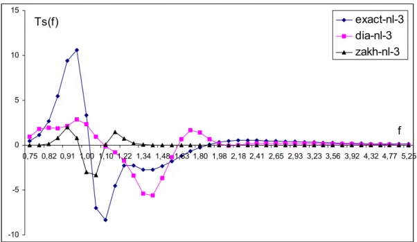
Fig. 3.The same as in Fig. 2 but for the run 3.
2. The greatest errors take place for very narrow (in fre-quency and in angular spreading) spectra (runs 3, 4) which are typical in developing waves. This effect is proved by a special consideration of 4 cases with swell second mode (runs 13–16) (mixed sea cases). In the
lat-ter cases, MRE (10%) for DIA can reach 100% (for 1-D
N L-transfer).
Table 2.MRE for 2-D-N land 1-D-N ltransfers in DIA No. of run Type of NL-transfer Adjusting coefficient Cad
MRE(10%), percents
MRE(20%), percents
1 2D-Nl
1D-Nl
1.37 22.0
19.7
0.166
2 2D-Nl
1D-Nl
1.25 35.9
21.7
20.9
3 2D-Nl
1D-Nl
1.33 68.9
70.2
78.6
4 2D-Nl
1D-Nl
2.44 73.3
69.8
56.1
5 2D-Nl
1D-Nl
1.21 36.2
82.7
24.3
6 2D-Nl
1D-Nl
1.13 41.6
71.8
36.1
7 2D-Nl
1D-Nl
1.31 46.7
57.4
30.2
8 2D-Nl
1D-Nl
1.52 35.2
25.3
24.2
9 2D-Nl
1D-Nl
1.17 49.0
45.5
30.0
10 2D-Nl
1D-Nl
1.49 43.4
76.2
44.6
11 2D-Nl
1D-Nl
1.44 40.3
29.3
31.6
12 2D-Nl
1D-Nl
1.69 24.4
51.1
15.9
13 2D-Nl
1D-Nl
1.32 64.5
92.7
69.9
14 2D-Nl
1D-Nl
1.35 51.5
90.7
60.2
15 2D-Nl
1D-Nl
1.33 64.7
93.7
69.9
16 2D-Nl
1D-Nl
2.81 68.1
108
46.4
can be introduced for the practical aims as a mean value of MRE for the representative set of spectrum shapes. On the basis of these conclusions we can propose the follow-ing recommendations.
1. The most representative set of spectrum shapes, which can be proposed for the next elaboration of DIA, should include runs 1, 2 and runs 3–7, 15, 16. The former two are considered as cases typical for the spectrum of de-veloped wind waves, while the latter are cases where the spectrum shape is of developing and mixed sea type. 2. With respect to DIA efficiency, the most appropriate
value of the relative error provided by DIA for 2-D-N l
can be accepted as a simple averaging of MRE (10%) through the 9 representative cases mentioned above. The “expert” estimation is
εrel(DI A)∼=0.5. (40) 3. Regarding DIA implementation, the “expert” value of
Cadis of the order of 1.6, which is in a good agreement with recommendations of the WAM group (Komen et al., 1994).
5.2.2 Zakharov-Puchkarev’s diffusion approximation From Table 3 one can see the following:
Table 3.MRE for 2-D-N land 1-D-N ltransfers in ZPA
No. of run
Type of
NL-transfer
Adjusting coefficient Cad
MRE(10%), percents
MRE(20%), percents
1 2D-Nl
1D-Nl
0.262 75.9
80.9
61.6
2 2D-Nl
1D-Nl
0.115 66.2
70.3
58.7
3 2D-Nl
1D-Nl
0.0083 103
106
88.1
4 2D-Nl
1D-Nl
0.0085 91.8 90.3
84.7
5 2D-Nl
1D-Nl
0.0580 74.8 78.1
77.3
6 2D-Nl
1D-Nl
0.022 86.5
75.3
86.1
7 2D-Nl
1D-Nl
0.0344 83.6 90.1
83.2
8 2D-Nl
1D-Nl
0.108 66.9
75.7
62.2
9 2D-Nl
1D-Nl
0.031 84.8
92.0
84.9
10 2D-Nl
1D-Nl
0.023 94.0
104
85.7
11 2D-Nl
1D-Nl
0.131 75.9
88.4
71.5
12 2D-Nl
1D-Nl
0.153 64.8
76.8
60.4
13 2D-Nl
1D-Nl
0.0089 99.5 103
80.2
14 2D-Nl
1D-Nl
0.0164 89.7 99.9
71.2
15 2D-Nl
1D-Nl
0.0092 100
105
79.8
16 2D-Nl
1D-Nl
0.0111 77.1 73.1
77.6
1 2 3 4 5 6 7 8 9 10 11 12 13 14 15 16
DIA 0 20 40 60 80 100 120 DIA ZPA MRE, %
Fig. 4.Comparative diagram of relative errors for the original DIA and ZPA. In horizontal axes the number of run from Table 1 is pre-sented.
– The relative errors for ZPA are greater than errors for DIA (in 1.5–2 times approximately), except of runs 5 and 10 for 1-DN L-transfer. A comparative diagram of errors for these two cases is presented in Fig. 4.
situations take place: cases 5 and 9.
– Variation of values for MRE (10%) due to dependence on the spectrum is rather remarkable:
– 64%≤MRE (10%)≤103% for 2-DN L-transfer,
– 70%≤MRE (10%)≤106% for 1-DN L-transfer.
– Variation of values for the adjusting coefficientCaddue to dependence on the spectrum is very essential: 0.26
≤Cad ≤0.0083.
On the basis of the presented results for ZPA, the following conclusions may be drawn.
1. The relative errors for ZPA are greater than errors for DIA in 1.5–2 times approximately, and their values de-pend strongly on the spectral shape (Fig. 4).
2. The adjusting coefficient depends very strongly on the shape of the spectrum under consideration. It seems that there is not any reasonable coefficientCad, which can be used as the appropriate one for all the spectral shapes in this approximation.
3. From the point of view of accuracy and stability of val-ues forCad, ZPA is less preferable than DIA.
Despite of the last conclusion, some practical recommenda-tions can be given.
1. With respect to the ZPA efficiency, the “expert” value of the relative error for 2-DN L-transfer (averaged through the 9 representative runs) can be accepted of the order of 85%, i.e.
εrel(ZP A)∼=0.85 (41)
2. In the case where ZPA is needed for practical use in numerical modeling, the most acceptable value forCad could be of the order of 0.05, according to recommen-dation given in Polnikov (2002).
5.3 Estimations of efficiency for DIA and ZPA
Due to the relatively long time of theN L-term calculations in DIA, the second type of efficiency given by Eq. (25) is more relevant to our analysis. To estimate efficiency, in addition to the estimation of relative error, we need proper estimations of the non-dimensional parameterstrel≡(Tref/τ )andRP. We have used a COMPAQ workstation forN L-term calcula-tions and supercomputer NEC SX-4 for WAM (Cycle 4) ap-plication. The former was used for estimation oftrel by the procedure SECNDS, while the latter was used for estimation ofRP by the software PROFILE.
The procedure of efficiency estimation and results are as follows.
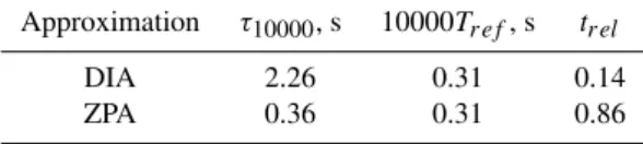
Table 4.Time parameters for DIA and ZPA
Approximation τ10000, s 10000Tref, s trel
DIA 2.26 0.31 0.14
ZPA 0.36 0.31 0.86
In fact, the following three codes are used in the effi-ciency estimation procedure. (1) A specially prepared one-configuration DIA adjusted to the integrating grid (“fast DIA”) is used for estimation ofTref; (2) An original DIA (or ZPA) approximation is used for estimation of the proper value ofτ; (3) The WAM (Cycle 4) is used for estimation of
RP.
To estimateTref, we have excluded the interpolation pro-cedures and the functional derivative part from the original DIA (fast DIA)11. After this we have estimated the CPU-time for 10000 cycles of the fast DIA. This CPU-time is just an estimation of the value 10000Tref.
Real one-step time,τ, for DIA and ZPA is estimated by the same “10000-step procedure” but for the original DIA-code (without the functional derivative part) and for our own ZPA-code. By this way we estimate an auxiliary value,τ10000 = 10000τ. Finally we have found the estimations presented in Table 4.
The relative part RP is estimated by the use of the PROFILE-procedure applied to the WAM (Cycle 4). For the total original DIA, the real value ofRP(DI A) is of the order of 0.45. For the present calculations of theN L-term only (without functional derivative), one may estimate the value ofRP(DI A) to be equal to 1/3 which is properly less that one known for the total DIA. Thus, the rest part of WAM takes about 65% of the whole time of wave forecast-ing. Note that this part of calculation time is not changed while changingN L-term approximation. Taking in mind the ratioτ10000(DI A)/τ10000(ZP A) ∼=6 following from Table 4, it is easy to calculate that the proper value ofRP(ZP A)is of the order of 1/13. So, we have all needed parameters for estimations of efficiency for the approximations under consideration.
According to Eqs. (25), (40), and (41), the efficiency for the DIA and ZPA approximations is
Eff2(DI A) =(1/0.5)2(0.14)1/3∼=2; (42)
Eff2(ZP A)=(1/0.85)2(0.86)1/13 ∼=1.4. (43) Thus, despite the relatively high speed of ZPA calculation of theN L-term, the real efficiency of DIA is greater due to its better accuracy.
mation of theN L-term is lying in the direction of the choice of optimal configurations for interacting waves, i.e. in the di-rection of improving DIA. Several variants of improvements of DIA will be considered in the following section.
6 Examples of improved DIA
As can be seen from the estimations in Sect. 5, there are es-sentially two ways for improving DIA: (1) to enhance the speed (and accuracy) of calculation for one-configuration DIA, or (2) to enhance an accuracy of approximation by adding new configurations (multiple DIA). Here we shall give two examples of improved DIA using these ways. 6.1 Fast DIA adjusted to the integration grid
As was mentioned in Sect. 2.1, the technical shortage of the original (one-configuration) DIA used in WAM is the pres-ence of intermediate and cumbersome interpolation proce-dures provided by a mismatch of the integration grid and the vectors k+,k−, which leads increase of computation time. Thus, to enhance a speed of calculation in a one-configuration DIA, one could adjust the one-configuration of in-teracting waves to the integration grid, and thus, avoiding interpolation. It can be done in the following way.
Instead of configuration (10) we propose to use the follow-ing:
1. k4=k, where the arbitrary wave vectorkis located at a grid node and represented in the polar co-ordinates by
σandθ;
2. k3=k+wherek+is represented by
σ3=σ (1+α34)andθ3=θ+1θ34; (44) 3. k1≈k2 ≈(k4+k3)/2 ≡kawherekais represented
by
θa=θ+1θa4.
The choice of the latter two vectors depends on the values of the parametersσ34and1θ34 defining vectorsk3andka. To solve the problem posed, one needs to meet the following requirements: (a) to preserve approximately the original DIA configuration, (b) to allocate all the vectors at the grid nodes, and (c) to chose values ofα34and1θ34in such a manner that the interacting vectors are allocated at the “figure-of eight” in thek-space (see Fig. 1).
The first requirement (original DIA configuration) can be expressed numerically as follows
α34 ≈1.5, σ1≈σ2, and 1θ34=45◦. (45) The second requirement (allocation of vectors at the grid nodes) is expressed by the following Fortran statements
Mod(θ34, 1θg)≪1θg, (46)
Mod(θa4, 1θg)≪1θg,
1 2 3 4 5 6 7 8 9 10 11 12 13 14 15 16
fa
st D
IA
0 10 20 30 40 50 60 70 80
fast DIA orig. DIA MRE, %
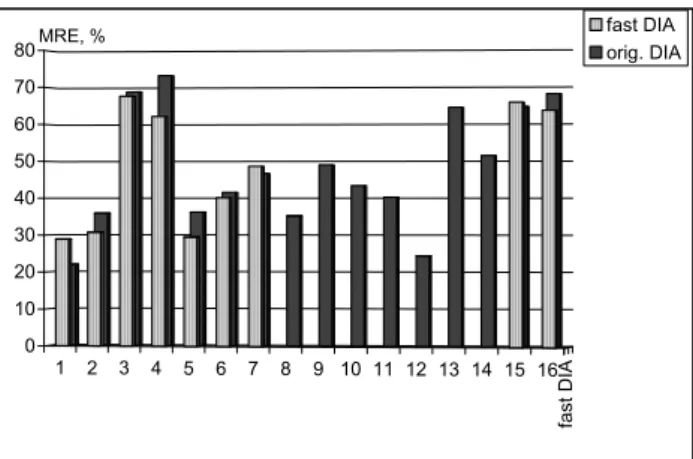
Fig. 5.Comparative diagram of relative errors for the fast and orig-inal DIA. For legend see Fig. 1.
and by the mathematical expressions
σ3/σ ≈em3, σ1/σ ≈em1, σ2/σ ≈em2. (47) In Eqs. (46)and (47),eis the frequency grid exponent,1θg is the angle grid resolution (see Eqs. 35 and 36), and powers
m1,m2,m3 are integer values to be found.
The third requirements (allocation at the “figure-of eight”) is expressed by the ratio (Polnikov, 1989):
ka=σa2/2, (48)
where
ka= h
σ4+σ34+2σ2σ32cos(1θ34) i1/2
(49) and
σa=σ+σ3. (50)
The expression for1θ34is deduced from the resonant condi-tion (5),
1θa4= arctg "
σ32sin(1θ34) σ32cos(1θ34)+σ2
#
. (51)
To meet all three requirements simultaneously, it is suffi-cient to fit properly a value ofm3 in Eq. (47) for the fixed grid parameterseand1θg. In the case of a reasonable grid resolution, the proper values ofm1,m2,m3,1θa4, and1θ34 can be found without any difficulties. In particular, for the grid given by Eqs. (35) and (36), we have
m3=10, ml=5, m2=6;
Table 5.MRE forN L-transfer in fast DIA with WAM-configuration
No of run 1 2 3 4 5 6 7 15 16
Coeff.Cad 1.99 1.56 2.11 2.83 1.57 1.48 1.89 1.90 3.2
MRE(10%) 28.9 30.8 67.6 62.1 29.5 40.1 48.6 65.7 63.5
MRE(20%) 20.9 20.3 66.5 51.2 24.8 30.8 29.0 63.5 39.7
MRE(10%)
For 1D-NL
26.3 17.5 66.3 56.4 75.6 74.8 56.7 80.9 100
Final results of the mean relative errors for the represen-tative set of spectral parameters are presented in Table 5 and Fig. 5.
From Fig. 5 it is seen that the fast one-configuration DIA has better features with respect to original DIA. In essence, we mention only that the expert MRE in this case is
εrel(f ast DI A)∼=0.48 (53) whilst the relative speed has the maximum possible value
trel(f ast DI A)=Tref/τ =1. (54) From Eqs. (54) and (24), (25) it follows that one should use the first type of efficiency. Finally, the efficiency of the ap-proximation under consideration is of the order
Eff1=(1/0.48)2∼=4.3. (55) Thus, the proposed fast DIA with WAM-configuration has twice the efficiency of original DIA12.
6.2 Modified (multiple) DIA adjusted to integration grid As follows from above, the advantage of the fast WAM-configuration DIA is provided by the enhancement of speed of calculation only. To enhance the accuracy of approxima-tion, one should construct DIA with several configuration of interacting waves (the so-called multiple DIA, Van Vled-der et al, 2000). Here we represent one of such a multiple DIA with three configurations adjusted to the integration grid given by Eqs. (35) and (36) (3c-DIA).
The main idea of a multiple configuration DIA is to in-volve into the approximation of N L-term such configura-tions, which cover an interaction grid wider in frequency and angle space than it is done in the WAM-configuration. The simplest way is to vary the parametersα34 and1θ34 in Eq. (44). Herewith, one should take in mind the weights of the configurations,Bc, as it follows from Eq. (18). But this point can be easily done by a previous estimation ofBcfrom the exact integrand expressions presented in integral (17).13
By analogy with the procedure described in Eq. (44), in Sect. 6.1, we have found the following version of the 3c-DIA: 12An implementation of fast DIA into the WAM (Cycle 4) gives the value of RP about 25%. In details the point of modified DIA implementation will be discussed in another paper.
13From this point of view, the multiple DIA resembles RIA. But the difference is in the choice of configurations.
1 2 3 4 5 6 7 8 9 10 11 12 13 14 15 16
3c-DI
A
0 10 20 30 40 50 60
70 3c-DIA
fast DIA
MRE, %
Fig. 6. Comparative diagram of relative errors for the 3c-DIA and fast DIA. Only the expert set of runs from Table 1 is shown.
1. Configuration 1 is presented by ratios
m3=8, m1=4, m2=5;
I nt (1θ34/1θg)=3, I nt (1θa4/1θg)=2; (56)
2. Configuration 2 is given by Eq. (52)
m3=12, m1=5, m2=6;
I nt (1θ34/1θg)=4, I nt (1θa4/1θg)=3; (57)
3. Configuration 3 is presented by ratios
m3=12, m1=7, m2=7;
I nt (1θ34/1θg)=5, I nt (1θa4/1θg)=4; (58)
For these configurations the relative values of weights,Bc, are approximately equal to each other. The rest part of cal-culations in 3c-DIA is nearly the same as in the fast DIA (exception is the number of configurations). Results of test-ing the three-configuration DIA, given by Eqs. (56)–(58), are presented in Table 6 and Fig. 6 for the representative set of spectral parameters.
Table 6.MRE forN L-transfer in three-configuration DIA
No of run 1 2 3 4 5 6 7 15 16
CoefficientCad 0.78 0.63 1.06 1.07 0.62 0.57 0.73 0.85 1.07
MRE(10%) 25.2 28.8 53.8 37.6 28.9 37.4 41.6 49.9 52.6
MRE(20%) 17.1 19.5 49.8 40.3 24.9 28.3 26.2 45.2 37.3
MRE(10%)
for 1D-NL
18.6 20.9 62.8 52.6 62.4 65.9 55.4 69.9 85.1
respect to the original DIA (compare Figs. 5 and 6). In this case, the expert MRE is
εrel(3c−DI A)∼=0.39 (59) and the relative speed has the value
trel(3c−DI A)=Tref/τ =0.33. (60) From Eq. (60) it follows that one should use the second type of efficiency. By analogy with the said above in Eq. (37), above in Sect. 6.1, we may take a relative part RP of the order of 1/3. Finally, we find
Eff1∼=(1/0.39)2(0.33)1/3∼=4.4. (61) Comparing Eq. (55) and Eq. (61) gives that the proposed three-configuration DIA has nearly the same efficiency as the fast DIA with the WAM-configuration. Herewith, taking in mind the better accuracy, we may state that the former ap-proximation is preferable.
7 Conclusions
The problem of optimizing approximations of the kinetic in-tegral describing the rate of four- wave nonlinear interactions is not completely solved yet. However, at present it seems that this problem is very close to its solution. The ground for this statement is the finding of this work that all the most prospective approximations: Discrete Interaction Approxi-mation (DIA), Reduced Integration ApproxiApproxi-mation (RIA), and Diffusion Approximation (DA), have the same root. All of them are different modifications of the Discrete Interac-tion ApproximaInterac-tion. The only difference among them is the choice of configurations for the interacting waves. Thus, the solution of the problem is the proper choice of the interacting configurations in a modified DIA.
To make this choice, one needs a tool for estimation of ac-curacy and efficiency of an approximation. This tool includes formal procedures on how to estimate these two parameters. On the basis of several heuristic postulates, appropriate for-mulas were constructed in this paper. They are Eqs. (24) and (25) for the efficiency parameter,Eff, and Eq. (31) for the mean relative error of approximation,εrel.
The formulas mentioned above were used for comparative estimation of accuracy and efficiency of two approximations:
original DIA (WAM-configuration) and DA in Zakharov-Pushkarev’s version (ZPA). It was shown that despite the smaller computational time in ZPA, the accuracy and effi-ciency of DIA is higher.
Taking in mind that the technical shortage in the original DIA (Hasselmann et al., 1985) consists in the presence of an interpolation procedure aimed to solve a mismatch of the in-tegration grid nodes and interacting wave vectors, two mod-ification of DIA were proposed. The first is the so-called “the fast one-configuration DIA” (fast DIA), the second is the three-configuration DIA (3c-DIA). Both of them are ad-justed to the certain integration grid, to exclude the cumber-some interpolation procedure mentioned above. Owing to this feature, both new approximations have efficiency more than twice greater than the original DIA. Herewith, the fast DIA is quicker in calculation, but the 3c-DIA has more ac-curacy. Both of approximations proposed are feasible to be implemented into practice, and this point will be described in another paper.
Here we did not test RIA given by expression (16). Never-theless, one may state in advance, that due to similarity RIA to a multiple configuration version of DA, efficiency of RIA is expected to be smaller than one for the original DIA. This point may be verified later, if necessary.
Due to the fact that the found values of accuracy and ef-ficiency for the proposed modifications of DIA are far from their upper limits provided by the aim of practice, more effec-tive approximations could be constructed, in principle. This is the final task of the problem under consideration.
Acknowledgements. The authors are grateful to the administration
of CPTEC and CNPq for the funding this work. In part, this work was supported by the Russian Fund for Basic Research, project # 01-05-64580. We appreciate Gerbrant van Vledder for his remarks made during the reading of the proofs.
References
Barnett, T. P.: On the generation, dissipation and prediction of ocean wind waves, J. Geophys. Res., 73, 513–529, 1968. Efimov, V. and Polnikov, V.: Numerical modeling of wind waves,
Kiev, Naukova dumka Publishing House, 240, 1991.
Hashimoto, N.: Extension of the DIA for computing the nonlin-ear energy transfer of ocean gravity waves, Proc. Jap. Conf. On Coastal Egnineering, (in Japanese), 1999.
Hashimoto, N. and Kawagushi, K.: Extension and modification of the Discrete Interaction Approximation (DIA) for computing nonlinear energy transfer of gravity wave spectra, Proc. 4th Int. Symp. on Ocean Waves, Measurement and Analysis, WAVES-2001, 2001.
Hasselmann, K.: On the non-linear energy transfer in a gravity wave spectrum, Pt. 1. General theory, J. Fluid Mech., 12, 481–500, 1962.
Hasselmann, S. and Hasselmann, K.: A symmetrical method of computing the nonlinear transfer in a gravity wave spectrum, Hamburger Geophys. Einzelschrift, 52, 138, 1981.
Hasselmann, S., Hasselmann, K., Allender, K. J. and Barnett, T. P.: Computations and parameterizations of the nonlinear energy transfer in a gravity-wave spectrum. Part II, J. Phys. Oceanogr., 15, 1378–1391, 1985.
Jenkins, A. and Phillips, O. M.: A Simple Formula for nonlinear Wave-Wave Interaction, Intern. J. of Offshore and Polar Engi-neering, 11, 81–86, 2001.
Komen, G. J., Cavaleri, L., Donelan, M., et al.: Dynamics and Mod-eling of Ocean Waves, N.Y., Cambridge University Press, 532, 1994.
Lavrenov, I. V. and Polnikov, V. G.: A study of properties for non-stationary solutions of the Hasselmann’s kinetic equation, Izvestiya, Atmos. Oceanic. Phys., (English transl.), 37, 5, 2001. Lin, R. Q. and Perry, W.: Wave-wave interactions in finite depth
water, J. Geophys. Res., 104, 11 193–11 213, 1999.
Masuda, A.: Nonlinear energy transfer between wind waves, J. Phys. Oceanogr., 15, 1369–1377, 1980.
Polnikov, V. G.: Calculation of the nonlinear energy transfer through the surface gravity waves spectrum. Izv. Acad. Sci. SSSR, Atmos. Oceanic. Phys., (English transl.), 25, 896–904, 1989.
Polnikov, V. G.: Numerical solution of the kinetic equation for sur-face gravity waves, Ibid., (English transl.), 26, 118–123, 1990. Polnikov, V. G.: A third generation spectral model for wind waves,
Ibid., (English transl.), 27, 615–623, 1991.
Polnikov, V. G.: Numerical modeling of flux spectra formation for surface gravity waves, J. Fluid Mech., 278, 289–296, 1994. Polnikov, V. G.: Numerical modeling of the constant flux spectra
for surface gravity waves in a case of angular anisotropy, Wave Motion, 33, 271–282, 2001.
Polnikov, V. G.: A Basing of the Diffusion Approximation Deriva-tion for the Four-Wave Kinetic Integral and Properties of the Ap-proximation, Nonl. Proc. Geophys., 9, 3/4, 355–366, 2002. Resio, D. T.: The estimation of wind wave generation in a discrete
spectral model, J. Phys. Oceanogr., 11, 510–525, 1981. Resio, D. and Perry, W.: A numerical study of nonlinear energy
fluxes due to wave-wave interactions., J. Fluid Mech., 223, 603– 629, 1991.
The SWAMP group: Ocean wave modeling, N. Y. and L., Plenum press, 256, 1985.
WAMDI group: The WAM model – A third generation Ocean Wave Prediction Model, J. Phys. Oceanogr., 18, 1775–1810, 1988. Webb, D. J.: Non-linear transfer between sea waves, Deep Sea Res.,
25, 279–298, 1978.
Zakharov, V. E. and Filonenko, N. N.: The energy spectrum for stochastic oscillation of fluid’s surface, Dokl. Akad. Nauk., 170, 1292–1295, 1966.
Zakharov, V. E. and Smilga, A. V.: On quasi-one-dimensional spec-tra of weak turbulence, Sov. Phys. JETP, (English spec-transl.), 54, 701–710, 1981.
Zakharov, V. E. and Pushkarev, A.: Diffusion model of interacting gravity waves on the surface of deep fluid, Nonl. Proc. Geophys., 6, 1–10, 1999.
Van Vledder, G. Ph., Herbers, T. H. C., Jense, R. E., et al.: Mod-eling of nonlinear quadruplet wave-wave interactions in opera-tional model, Proc. 27th Int. Conf. Coastal Engineering, 2000. Van Vledder, G. Ph.: Extension of the Discrete Interaction
Approx-imation for computing nonlinear quadruplet wave-wave interac-tions in operational wave prediction model, Proc. 4th Int. Conf. on Ocean Waves. WAVES-2001. San Fransisco, Sept., 2001. Young, I. R. and Van Vledder, G. Ph.: The Central Role of