www.biogeosciences.net/12/4067/2015/ doi:10.5194/bg-12-4067-2015
© Author(s) 2015. CC Attribution 3.0 License.
Investigating the usefulness of satellite-derived fluorescence data in
inferring gross primary productivity within the carbon cycle data
assimilation system
E. N. Koffi1,a, P. J. Rayner2, A. J. Norton2, C. Frankenberg3, and M. Scholze4
1Laboratoire des Sciences du Climat et de l’Environnement (LSCE), UMR8212, Ormes des merisiers,
91191 Gif-sur-Yvette, France
2School of Earth Sciences, University of Melbourne, Melbourne, Australia 3Jet Propulsion Laboratory, California Institute of Technology, Pasadena, USA
4Department of Physical Geography and Ecosystem Science, Lund University, Lund, Sweden
anow at: the European Commission Joint Research Centre, Institute for Environment and Sustainability,
21027 Ispra (Va), Italy
Correspondence to:E. N. Koffi (ernest.koffi@jrc.ec.europa.eu)
Received: 01 December 2014 – Published in Biogeosciences Discuss.: 13 January 2015 Revised: 18 June 2015 – Accepted: 18 June 2015 – Published: 07 July 2015
Abstract. Simulations of carbon fluxes with terrestrial bio-sphere models still exhibit significant uncertainties, in part due to the uncertainty in model parameter values. With the advent of satellite measurements of solar induced chloro-phyll fluorescence (SIF), there exists a novel pathway for constraining simulated carbon fluxes and parameter values. We investigate the utility of SIF in constraining gross primary productivity (GPP). As a first test we assess whether SIF sim-ulations are sensitive to important parameters in a biosphere model. SIF measurements at the wavelength of 755 nm are simulated by the Carbon-Cycle Data Assimilation System (CCDAS) which has been augmented by the fluorescence component of the Soil Canopy Observation, Photochemistry and Energy fluxes (SCOPE) model.
Idealized sensitivity tests of the SCOPE model stand-alone indicate strong sensitivity of GPP to the carboxylation capac-ity (Vcmax) and of SIF to the chlorophyll AB content (Cab)
and incoming short wave radiation. Low sensitivity is found for SIF toVcmax, however the relationship is subtle, with
in-creased sensitivity under high radiation conditions and lower Vcmaxranges.
CCDAS simulates well the patterns of satellite-measured SIF suggesting the combined model is capable of ingesting the data. CCDAS supports the idealized sensitivity tests of SCOPE, with SIF exhibiting sensitivity to Cab and
incom-ing radiation, both of which are treated as perfectly known in previous CCDAS versions. These results demonstrate the need for careful consideration ofCaband incoming radiation
when interpreting SIF and the limitations of utilizing SIF to constrainVcmaxin the present set-up in the CCDAS system.
1 Introduction
The terrestrial carbon flux has been identified as the most uncertain term in the global carbon budget (Le Quéré et al., 2013). The gross primary productivity (GPP), which is the flux of CO2assimilated by plants during photosynthesis, is
the input to the system used to characterize carbon flux so its variation can significantly contribute to the uncertainties in terrestrial CO2fluxes.
Complex systems have been built to reduce the uncertain-ties in GPP. These algorithms are either based on up-scaling or atmospheric inverse modelling methods. Up-scaling meth-ods estimate GPP at global scale by establishing relation-ships between local GPP measurements and environmental variables then using these variables to calculate GPP glob-ally (e.g., Jung et al., 2011; Beer et al., 2010 and references therein). The inverse modelling approach uses CO2
pro-cess parameters of carbon models that compute the terrestrial fluxes. This inverse method is an example of Carbon Cycle Data Assimilation Systems (CCDAS). The CCDAS consid-ered in the present study has two main components:
– A deterministic dynamical model that computes the evolution of both the biosphere and soil carbon stores given an initial condition, forcing and a set of the model process parameters.
– An assimilation algorithm that allows the adjustment of a subset of the state variables, initial conditions and/or process parameters to reduce the mismatch between the model simulations and observations. Usually any prior information on the variables which are adjusted are also taken into account (see e.g., Kaminski et al., 2002, 2003; Rayner et al., 2005, and references therein for the underlying methodology).
Rayner et al. (2005) built such a CCDAS around the bio-sphere model BETHY (Biobio-sphere Energy-Transfer Hydrol-ogy; Knorr, 2000) coupled to an atmospheric transport model together with CO2 fluxes representing ocean flux, land
use change, and fossil fuel emission, see also Scholze at al. (2007) and Kaminski et al. (2013) for an overview on further developments and applications. Koffi et al. (2012) used this CCDAS to investigate the sensitivity of estimates of GPP to transport models and observational networks of CO2concentrations. Large differences in GPP in the tropics
were found between the GPP estimates of Koffi et al. (2012) and those from either satellite-based products or up-scaling methods (e.g., Jung et al., 2011; Beer et al., 2010). Koffi et al. (2012) found significantly larger GPP in the tropics com-pared to the other GPP products. In fact, due to few CO2
concentration observations available in the tropics, the pa-rameters of BETHY are mainly constrained by observations from other regions. Consequently, the optimized parameters can be uncertain.
Recent work has inferred sun-induced plant fluorescence (hereafter SIF) from the Greenhouse gas Observing Satel-lite (GOSAT; e.g., Frankenberg et al., 2011, 2012; Joiner et al., 2011; Guanter et al., 2012), ENVISAT/SCIAMACHY (Joiner et al., 2012), and MetOp-A/GOME-2 (Joiner et al., 2013). They showed that SIF data at a global scale is promis-ing for inferrpromis-ing GPP. They found a strong linear correlation between satellite-based SIF and GPP estimated from either up-scaling methods (Jung et al., 2011) or satellite products (MODIS data). The satellite-based SIF data cover large areas of the globe including tropical zones where estimates from a CCDAS are found to be uncertain. It is worth asking whether such fluorescence data is useful to constrain GPP in the CC-DAS framework.
The relationship between fluorescence and photochem-istry at leaf level is reasonably well understood. Light energy absorbed by chlorophyll molecules has one of three fates: photosynthesis, dissipation as heat (non-photochemical
quenching) or chlorophyll fluorescence. The total amount of chlorophyll fluorescence is only 1 to 2 % of total light ab-sorbed. The spectrum of fluorescence is different to that of absorbed light. The peak of the fluorescence spectrum lies between 650 and 850 nm. Under low-light conditions, a neg-ative correlation has been found between fluorescence and photosynthesis light use efficiencies (e.g., Genty et al., 1989; Rosema et al., 1998; Seaton and Walker, 1990; Maxwell and Johnson, 2000; van der Tol et al., 2009a). At high-light con-ditions (i.e., high irradiance and moisture stress), a positive correlation has been observed between fluorescence and pho-tosynthesis light use efficiencies (Gilmore and Yamamoto, 1992; Gilmore et al., 1994; Maxwell and Johnson, 2000; van der Tol et al., 2009a). Regarding the water stress, more re-cently, Lee et al. (2013) showed a negative correlation be-tween vapour pressure deficit and SIF.
The cited works above show that the link between fluores-cence and photosynthesis is complex. Thus, before using flu-orescence observations to constrain gross primary productiv-ity in the framework of CCDAS, first we need to ensure that there is a common parameter or set of parameters relevant to both the fluorescence and photosynthesis process models of the CCDAS. So, if there are common parameters, we can as-sess the sensitivities of GPP and SIF to them. This requires implementing in CCDAS a model that allows for the comput-ing of both fluorescence and photosynthesis. We build such a CCDAS by using the SCOPE (Soil Canopy Observation, Photochemistry and Energy fluxes) model (van der Tol et al., 2009a, 2014). SCOPE is based on the existing theory of chlorophyll fluorescence and photosynthesis. The photosyn-thesis scheme of C3 plants uses the formulations of Collatz et al. (1991), while for the C4 photosynthesis pathway, the formulations of Collatz et al. (1992) are considered. In these formulations of the photosynthesis, the maximum carboxyla-tion rateVcmaxis a key process parameter. The fluorescence
model is based on the work of Genty et al. (1989), Rosema et al. (1998), and van der Tol et al. (2014). The model is for-mulated such that the sum of the probabilities of an absorbed photon to result in fluorescence, photochemistry, and heat is unity. Hence, the fluorescence model also utilizesVcmaxas a
process parameter.
CCDAS operates in two modes (Scholze et al., 2007). The calibration mode that derives an optimal parameter set including posterior uncertainties of the dynamical carbon model (here the biosphere model) by constraining the pro-cess parameters of the model with observations. The diag-nostic/prognostic (referred hereafter as forward) mode al-lows deriving the various quantities of interest (e.g., terres-trial carbon fluxes or atmospheric CO2concentrations) and
the uncertainty in the parameters of BETHY by using both CO2concentration and flux observational networks
(Kamin-ski et al., 2012; Koffi et al., 2013). To assess the usefulness of satellite-based fluorescence data (SIF) to constrain GPP within CCDAS, in this study, we investigate the sensitivities of both GPP and SIF to the biochemical parameters as well as environmental conditions by using the SCOPE model alone and the forward mode of the CCDAS built around it. The work is organized as follows: in Sect. 2, we describe both the model SCOPE and its coupling with CCDAS and the fluo-rescence data retrieved from the satellite GOSAT. In Sect. 3, we perform various idealized sensitivity tests to investigate the strength of the relationships between SIF and GPP by us-ing the SCOPE model alone. These tests are performed by studying the sensitivity of GPP and SIF to the biochemical parameters (i.e.,Vcmaxand the chlorophyll AB contentCab)
and the environmental conditions (e.g., incoming short wave radiation Rin). In the idealized tests, the vegetation is
char-acterized by different values of the leaf area index (LAI). In Sect. 4, by using the forward mode of the CCDAS coupled to SCOPE, we compute both SIF and GPP at global scale and results are compared to the GOSAT SIF from June 2009 until December 2010. The simulations are based on the different settings of LAI,Rin,Vcmax, andCabvalues. In Sect. 5, results
are discussed. Finally, conclusions are presented in Sect. 6.
2 Models and data 2.1 Models
2.1.1 SCOPE model
The model SCOPE is a 1-D model based on radiative trans-fer, micrometeorology, and plant physiology (van der Tol et al., 2009b). Version 1.53 of SCOPE is used in this study with the default version of the biochemical code (referred as flu-orescence model choice 0; van der Tol et al., 2014). SCOPE treats canopy radiative transfer in the visible and infrared and chlorophyll fluorescence, as well as the energy balance. The modules of SCOPE are executed in the following order:
1. A semi-empirical radiative transfer model for incident sun and sky radiation, based on the SAIL model (Ver-hoef and Bach, 2007). This module calculates the out-going radiation spectrum (0.4 to 50 µm) at the top of the canopy (hereafter TOC), as well as the net radiation and absorbed photosynthetically active radiation (aPAR) per surface element.
2. A numerical radiative transfer model for thermal radia-tion generated internally by soil and vegetaradia-tion, based on Verhoef et al. (2007). This module computes the TOC outgoing thermal radiation and net radiation per surface element, but for heterogeneous leaf and soil temperatures.
3. A biochemistry model for C3 and C4 plants, which al-lows the computation of quantities relevant for photo-synthesis and chlorophyll fluorescence at leaf level. At leaf level, the model calculates a fluorescence scaling factor relative to that of a leaf in low-light, unstressed conditions from absorbed radiative fluxes, canopy and ambient environmental conditions (radiation, tempera-ture, air vapour pressure, CO2, and O2concentrations).
4. A radiative transfer model for chlorophyll fluorescence based on the FluorSAIL model (Miller et al., 2005) that calculates the TOC radiance spectrum of fluorescence over 640–850 nm from the geometry of the canopy and a calculated fluorescence spectrum that is linearly scaled by the leaf level chlorophyll fluorescence scaling factor. In this study, SCOPE uses a canopy structure characterized by a spherical leaf angle distribution (parameters LIDFaand
LIDFbin Table 1) as a function of LAI with 60 distributed
elementary layers. The geometry of the vegetation is treated stochastically. SCOPE calculates the illumination of leaves with respect to their position and orientation in the canopy. The spectra of reflected and emitted radiation as observed above the canopy in the satellite observation direction are computed. It is worth noting that SCOPE permits variation only in the vertical dimension. Thus, it is valid for vegeta-tion in which variavegeta-tions in the horizontal are smaller than in the vertical dimension. This is maybe a limitation for some natural canopies, especially when coupling to the CCDAS as performed in Sect. 2.1.2. However, the sensitivity of this limitation to the CCDAS results is beyond the scope of this study.
We briefly describe the fluorescence model at leaf level (more detail is given in van der Tol et al., 2009a, 2014) with focus on the variables and parameters relevant for the photo-synthesis. The model of Faquahar et al. (1980) divides pho-tosynthesis into two main processes: (1) regeneration of the ribulose bisphosphate (RuP2), which depends on the light and (2) the maximum carboxylation rate at RuP2 saturated conditions in the presence of sufficient light. The regenera-tion of RuP2 for two photosystems (PSII and PSI) gives the link between photosynthesis and fluorescence.
As already mentioned above, the fluorescence model in SCOPE is formulated such that the sum of the probabilities of an absorbed photon to result in fluorescence, photochemistry, and heat is unity. Following this, the fluorescence8Ft from
a single leaf is calculated over the spectrum window of 640– 850 nm as follows:
8Ft=8Fm 1−8p, (1)
where8Fm is the fluorescence yield and computed as
fol-lows:
8Fm= Kf
WithKnbeing the rate coefficient relative to nonphotochem-ical quenching (NPQ), a parameter obtained from Pulse am-plitude modulated (PAM) fluorometry. PAM measures the photosynthetic efficiency of photosystem II (PSII). Kn is parametrized by using Flexas et al. (2002)’s data set as fol-lows:
Kn=(6.2473×x−0.5944)×x, (3)
wherexstands for the degree of light saturation and defined as:
x=1− 8p
8p0
. (4)
8p and8p0 (given by the following expressions) stand for
the fractions of actual and dark photochemistry yields, re-spectively:
8p0= Kp
Kf+Kd+Kp
. (5)
Kfis the rate constant for fluorescence and sets to 0.05,Kpis
the rate constant for photochemistry with a value of 4.0,Kd,
with a value of 0.95, is the rate constant for thermal deacti-vation at8Fm
8p=8p0Ja Je
. (6)
JaandJestand for the actual and potential electron transport
rates, respectively. Jais the electron transport rate used for
gross primary productivity (GPP). van der Tol et al. (2014) used Pulse-Amplitude fluorescence measurements to derive an empirical relation between the efficiencies of photochem-istry and fluorescence. This relationship was derived af-ter analysing the response of non-photochemical quenching (NPQ) in plants to light saturation. The formulations of GPP in SCOPE follow that of Collatz et al. (1991) and Collatz et al. (1992) for C3 and C4 plants, respectively. The potential electron transport rate Je is related to the rate of absorbed
photons (or absorbed photosynthetically active radiation, i.e. aPAR), hence to the visible radiation. The fluorescence is lin-early related to the short wave (visible) radiation, while it is related toVcmaxmainly when the gross primary productivity
GPP is limited by the carboxylation enzyme Rubisco and the capacity for the export or the utilization of the products of photosynthesis.
The total top-of-canopy fluorescent radiance is obtained from the fluorescence flux (i.e.,8Ft in Eq. 1) and the
spec-tral radiance of single leaves over all layers and orienta-tions, taking into account the probabilities of viewing sun-lit and shaded components. The model then calculates radi-ation transport in a multilayer canopy as a function of the solar zenith angle and leaf orientation to simulate fluores-cence in the direction of satellite observation (van der Tol et al., 2009b).
Leaf biochemistry affects reflectance, transmittance, tran-spiration, photosynthesis, stomatal resistance, and chloro-phyll fluorescence. Reflectance and transmittance coeffi-cients, which are a function ofCabare calculated by
follow-ing the PROSPECT model (Jacquemoud and Baret, 1990). Two excitation fluorescence matrices (EF-matrices) repre-senting fluorescence from both sides of the leaf are com-puted. The matrices convert a spectrum of aPAR into a spec-trum of fluorescence. Details on the radiative transfer model of the fluorescence at the TOC level are given in van der Tol et al. (2009b).
2.1.2 Coupling SCOPE to CCDAS
Within CCDAS we replace the canopy radiative transfer and photosynthesis schemes of BETHY with their correspond-ing schemes from SCOPE and add the fluorescence model of SCOPE. The spatial resolution, vegetation characteristics as well as the meteorological and phenological data of BETHY are used to force SCOPE. The spatial resolution is 2◦
×2◦
with 3462 land grid points for the globe. CCDAS uses 13 plant functional types (PFT; see Table 2), which have been derived by a condensation (grouping different crop types into one crop PFT) of the original 23 PFTs in BETHY (Knorr, 1997, based on Wilson and Henderson-Sellers, 1985). A grid cell can contain up to three different PFTs, with the amount specified by their fractional coverage.
2.2 Data
2.2.1 GOSAT fluorescence data
Frankenberg et al. (2011, 2012), Joiner et al. (2011), and Guanter et al., (2012) have published maps of SIF from GOSAT (Kuze et al, 2009). The retrieval measures terrestrial emission at the frequencies of solar Fraunhofer lines (gaps in the solar spectrum). Chlorophyll fluorescence is the main contributor to emissions at these frequencies. GOSAT car-ries a Fourier Transform Spectrometer (FTS) measuring with high spectral resolution in the 755–775 nm range, which al-lows resolving individual Fraunhofer lines overlapping the fluorescence emission. The method described in Frankenberg et al. (2011) makes use of two spectral windows centred at 755 and 770 nm to derive SIF. Results from the line centred around 755 nm for the period June 2009 to December 2010 are used in this study. The fluorescence data we are using are monthly means mapped onto 2◦× 2◦ spatial resolution at global scale. The fluorescence product includes uncertain-ties.
2.2.2 Data relevant for models
Table 1.SCOPE parameters.
Parameters Symbol Units Range or values
Incoming short wave radiation Rin W m−2 0–1200
Maximum carboxylation rate Vcmax µmol m−2s−1 1–250
Chlorophylla+bcontent Cab µg cm−2 1–80
Dry matter content Cdm g cm 0.012
Leaf equivalent water thickness Cw cm 0.009
Senescent material Cs / 0.0
Leaf structure N / 1.4
Leaf angle distribution parametera LIDFa / −0.35
Leaf angle distribution parametera LIDFb / −0.15
Leaf width w m 0.1
Ball-Berry stomatal conductance parameter m / 8
Dark respiration rate at 25◦C as fraction of
Vcmax Rd / 0.015
Cowan’s water use efficiency parameter kc / 700
Leaf thermal reflectance ρ(thermal) / 0.01
Leaf thermal transmittance τ(thermal) / 0.01
Soil thermal reflectance ρs(thermal) / 0.06
Leaf area index LAI / 0.1–6
fluorescence quantum yield efficiency at photosystem level fqe / 0.02
Canopy height hc m 1
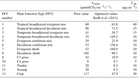
Table 2.Main controlling parameters for the photosynthesis and fluorescence models are given.Vcmaxstands for carboxylation maximum capacity andCabfor the chlorophyll AB content for 13 plant functional types (PFT) as used in the CCDAS.
Vcmax Cab
(µmol(CO2) m−2s−1) (µg cm−2)
PFT Plant Function Type (PFT) Prior value Optmized values
number Koffi et al. (2012)
1 Tropical broadleaved evergreen tree 60 63.8 40
2 Tropical broadleaved deciduous tree 90 73.5 15
3 Temperate broadleaved evergreen tree 41 39.7 15
4 Temperate broadleaved deciduous tree 35 149.2 10
5 Evergreen coniferous tree 29 21.9 10
6 Deciduous coniferous tree 53 136.4 10
7 Evergreen shrub 52 168.9 10
8 Deciduous shrub 160 96.1 10
9 C3 grass 42 18.9 10
10 C4 grass 8 0.7 5
11 Tundra 20 8.5 10
12 Swamp 20 9.3 10
13 Crop 117 47.9 20
relevant for both the canopy radiative transfer and istry models, and (iii) the process parameters of the biochem-istry models.
The model SCOPE requires incident radiation at the top-of-canopy as input. To take into account the atmospheric ab-sorption bands properly, these data are needed at high res-olution. The spectra of sun and sky fluxes at the top of the canopy are obtained from the atmospheric radiative transfer model MODTRAN (Berk et al., 2000). MODTRAN was run for 16 atmospheric situations representative of different
ide-Figure 1.The simulated fluorescence (SIF) at the top of the canopy as a function of the radiation wavelength and for C3 (black solid line) and C4 (red dashed line) plants from the model SCOPE are shown, respectively. The blue solid line corresponds to wavelength value (i.e., 755 nm) at which the simulated SIF is calculated in this study, i.e., the equivalent of the satellite GOSAT based SIF.
alized tests (Sect. 4.1) and the seasonal atmosphere for the simulations at global scale by using the CCDAS (Sect. 4.2).
The system needs forcing data to drive SCOPE within the CCDAS framework. Monthly observed climate, incident radiation, and fractional soil moisture for the period 2009– 2010 are used (Weedon et al., 2011). The LAIs are obtained from BETHY simulation.
The main parameters that affect both the photosynthe-sis and fluorescence schemes are given in Table 2. The pa-rameters are of two kinds: papa-rameters that are PFT-specific (e.g., Vcmax andCab) and global parameters. Prior and
op-timized values of Vcmax obtained by Koffi et al. (2012) are
shown. The chlorophyll content Cab is related to the
nitro-gen content of the leaf which itself is linked to the maximum rate of carboxylation through the proteins of the Calvin Cy-cle and the thylakoids. Some investigators have related the photosynthetic capacity of leaves of some specific plants to their nitrogen content (e.g., Evans, 1989; Kattge et al., 2009; Houborg et al., 2013). Other investigators have derived some empirical relationships between the nitrogen content and the chlorophyll content (e.g., Shaahan et al., 1999; van den Berg and Perkins, 2004; Ghasemi et al., 2011). Since the current version of the model SCOPE does not include the nitrogen scheme of a leaf, we first use the same value of chlorophyll contentCabfor all 13 PFTs. As a second step,Cabvalues for
each of the 13 PFTs are optimized so that the simulated SIF reproduces the main spatial characteristics of observed SIF.
3 Experimental set ups 3.1 Idealized tests
We carry out some idealized sensitivity tests by using the SCOPE model alone. We investigate the sensitivity of SIF and GPP to biochemical parametersVcmaxandCab,
environ-mental variables (atmospheric temperature and vapour pres-sure, etc), visible radiation, and LAI. We assume throughout the following sections the concentrations of both CO2 and
O2 at the interface of the canopy to be constant. We will
focus our discussions on the assessment of the sensitivity of the simulated SIF and GPP toVcmax,Cab, LAI, and the
short wave radiation. All the simulations in these tests are performed at noon.
We present a spectrum of simulated fluorescence for C3 and C4 plants in Fig. 1. Two peaks in the simulated fluo-rescence spectrum are shown at 680 and 725 nm. In agree-ment with van der Tol et al. (2009a), C4 plants exhibit larger SIF than C3 plants over the wavelength range 625 to 755 nm. These differences are amplified around the two peaks. We are using as observations the GOSAT satellite-derived SIF, which retrieved SIF around 755 nm. Therefore, the simulated fluorescence in this study corresponds to the SIF value at this wavelength. In Fig. 1, this is around 1.2 Wm−2µm−1sr−1.
For all of the idealized tests presented hereafter, we use eight values of LAI: 0.1, 0.5, 1, 2, 3, 4, 5, and 6. Also, the pressure, the temperature, and the vapour pressure of the air surrounding the leaf used to compute the internal CO2
con-centration of the leaf are set to 1000 hPa, 25◦C, and 10 hPa, respectively. The carbon dioxide (CO2) and the oxygen (O2)
concentrations are set to 355 ppm and 210×103ppm,
re-spectively. The other settings of SCOPE relevant for this study are given in Table 1.
– To investigate the sensitivity of SIF and GPP to the max-imum carboxylation capacityVcmax, we choose Vcmax
values ranging from 10 to 250 µmol(CO2) m−2s−1
ev-ery 10 µmol m−2s−1. In addition, two smallV
cmax
val-ues of 0.5 and 5 µmol m−2s−1are considered.
– To study the sensitivity of SIF and GPP to the chloro-phyll AB content (Cab), we selectCabvalues that span
10 to 80 µg cm−2range every 5 µg cm−2. Additionally, a smallCabvalue of 1 µg cm−2is considered.
– To assess the sensitivity of the SIF and GPP to the broadband incoming shortwave radiation (0.4–2.5 µm; hereafter Rin) at the top of the canopy, we select Rin values that range from 100 to 1200 W m−2 every
100 W m−2. We add small values of 1, 5, 10, 25, 50, and 75 W m−2.
latitude and 24.29◦longitude), which is one of the sites of the FLUXNET network (e.g., Baldocchi, 2003; Pa-pale et al., 2006; see the dedicated website: http://www. fluxnet.ornl.gov). SCOPE GPPs are compared to the ob-servationally derived GPP data. Unfortunately, we do not have observed SIF for this period.
3.2 CCDAS simulations
Since the idealized tests may give a partial picture of the re-lationship between SIF and GPP, we use the CCDAS built around SCOPE to perform additional sensitivity tests by us-ing actual meteorological, radiation, and phenological data over 2009–2010. Overall, the values of the short wave ra-diationRin used in the CCDAS are mostly under moderate
light conditions (around 400–600 W m−2), but at some pix-elsRinvalues can be larger than 800 W m−2(see Sect. S3 in
the Supplement). The relationship between SIF and GPP is then investigated along withVcmax andCab. We make
sim-ulations of SIF and GPP by using prior values ofVcmaxand
their optimized values from Koffi et al. (2012). We also carry out simulations by using a constant value ofCabfor all the 13
PFTs and a set ofCabvalues for each of them. We perform
four experiments (i.e., S1 to S4), which are summarized in Table 3. The experiments S1 and S3 use a constant value of Cabfor all of the 13 PFTs, while simulations S2 and S4
considerCab to be PFT dependent (Cabvalues are reported
in Table 2). The experiments S1 and S2 consider the prior values ofVcmax, while S3 and S4 their optimized values. The
differences between S1 and S3 or between S2 and S4 give the sensitivity of SIF and GPP toVcmax. The differences between
S1 and S2 or between S3 and S4 mainly give the sensitivity of SIF toCab.
The CCDAS simulates hourly SIF and GPP for one repre-sentative day in a month. Since the computation of fluores-cence is time consuming, we compute both SIF and GPP only at 12 h local time, i.e., around the time of their peaks during a sunny day. For the simulated SIF, the computations are as-signed to the 15th day of the month by using the monthly climate data and phenological variables of BETHY, as de-scribed in Sect. 2.2.2. We also neglect the energy balance scheme in SCOPE which weakly affects SIF.
4 Results
4.1 Idealized sensitivity tests using SCOPE
The results of these idealized sensitivity tests for the various LAI values are summarized in Figs. 2 and 3. For clarity, re-sults from C3 plant are discussed. Then, some conclusions are given for C4 plant.
Figure 2.The sensitivities of SCOPE fluorescence (SIF) at the top of the canopy ofC3plant to the carboxylation maximum capacity (Vcmax), chlorophyll AB content (Cab), and to the broadband in-coming shortwave radiation (0.4-2.5 µm) (Rin) for several leaf area indices (LAI) are shown. Graphs (aandb) stand for SIF and GPP as function ofVcmax, respectively. Graphs (candd) give the
sensi-tivities of SIF and GPP toCab, respectively. Graphs (eandf) show SIF and GPP as a function ofRin, respectively.
4.1.1 Sensitivity of SIF and GPP to biochemistry parameters
Figure 2 shows the sensitivity of both SIF and GPP to LAI,Vcmax, andCabunder moderate light conditions (Rin=
500 W m−2). As expected, both the fluorescence SIF and GPP increase with the increase of LAI (Fig. 2). However, a weak sensitivity is found for LAI values greater than 4. As an illustration for the increase, forVcmax=50 µmol m−2s−1,
SIF values of 0.5 and 1.25 W m−2µm−1sr−1are found for LAI of 0.5 and 2, respectively (Fig. 2a). The fluorescence slightly increases with an increase ofVcmax. The
sensitiv-ity is relatively large forVcmax, less than 70 µmol m−2s−1.
Then, SIF remains almost constant for Vcmax higher than
125 µmolm−2s−1 (Fig. 2a). As an illustration, for LAI
=2,
the largest increase is of only 50 % of SIF forVcmaxbetween
10 and 70 µmol m−2s−1. Under the studied configurations SIF increases withVcmaxwhen the GPP is controlled by the
Table 3.Set-ups for the CCDAS simulations based on the carboxylation maximum capacity (Vcmax) and chlorophyll AB content (Cab) are given. The values of prior and optimizedVcmaxas well asCabPFT-specific are given in Table 2. The constant value ofCabfor all 13 PFTs is set to 40 µg cm−2.
Model configuration Vcmax Cab
S1 Prior values Constant value for all the 13 PFTs
S2 Prior values CabPFT-specific
S3 Optimized values Constant value for all the 13 PFTs S4 Optimized values CabPFT-specific
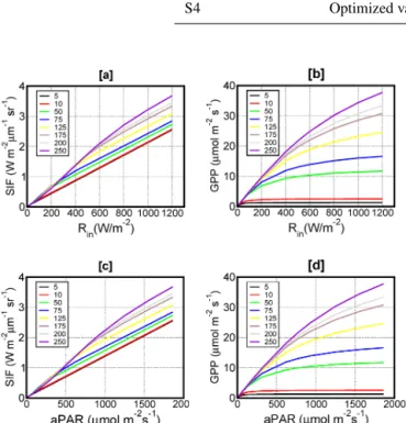
Figure 3.The sensitivities of the SCOPE fluorescence SIF (aand
c) and gross primary productivity (GPP) (bandd) to the incoming short wave radiation (Rin) and absorbed photosynthetically active radiation (aPAR) and for severalVcmaxare presented. LAI andCab are set to 2 and 40 µg cm−2, respectively. Results for aC
3plant are shown.
GPP monotonically increases as Vcmax increases with
large sensitivity for smallVcmax(less than 75 µmol m−2s−1),
then it becomes weakly sensitive for large values ofVcmax
(Fig. 2b). A moderate positive correlation is found between SIF and GPP forVcmaxless than 125 µmol m−2s−1, as shown
by the increase of both SIF and GPP with Vcmax (Fig. 2a
and b). Then, for larger Vcmax (i.e., 125 µmol m−2s−1), a
very weak negative correlation between SIF and GPP is ob-tained. The reason for this weak negative correlation is that SIF slightly decreases for largeVcmax, while GPP even
lim-ited by the carboxylation enzyme Rubisco still slightly in-creases (Fig. 2a and b). In fact, the value of irradiance at which the fluorescence yield at leaf level 8Ft (Eq. 1) or
SIF peaks increases with the increase of Vcmax. Thus, for
the case presented in Fig. 2a with the short wave radia-tion Rin of 500 W m−2, the peak of SIF occurs at about Vcmax=200 µmol m−2s−1.
In the current version of the fluorescence model in SCOPE, the concentration of chlorophyllCabis set as a
pa-rameter and it is linked to SIF through the transmittance and reflectance of the leaves. Figure 2c portrays the variations of SIF as a function ofCaband for various LAIs. For a given
LAI, SIF increases withCabwith large sensitivity forCabless
than 20 µg cm−2. For largerC
abvalues (i.e.,>50 µg cm−2),
SIF remains almost constant with a tendency to slightly de-crease asCabincreases. For a givenCab, the variance in SIF
due to the LAI can be significant.
Fig. 2d displays GPP as a function ofCab(Fig. 2d). Except
for small values ofCab(less than 5 µg cm−2), GPP is not
sen-sitive toCab. The very weak sensitivity of GPP toCabcomes
from the impact of the chlorophyll content on the transmit-tance and reflectransmit-tance at the top of the canopy when comput-ing the aPAR. This lack of sensitivity of GPP toCab
con-tradicts the established positive relationship between the two variables as reported in Fleischer (1935) and more recently in Gitelson et al. (2006).
4.1.2 Sensitivity of SIF and GPP to short wave radiation
For a given LAI, both SIF and GPP increase with the top of canopy short wave radiation (Rin) (Fig. 2e and f). Thus,
a strong positive linear correlation is obtained between SIF andRin(Fig. 2e), while a non-linear (i.e., curvilinear)
rela-tionship is obtained between GPP andRin(Fig. 2f). For large Rin, GPP increases with a slower rate indicating that the
pho-tosynthesis is limited by the carboxylation enzyme Rubisco. For the selected values of LAI, large variance is found be-tween SIF andRin(Fig. 2e). We also investigate the
relation-ship between the simulated aPAR and both computed SIF and GPP (see Sect. S1 in the Supplement). As expected, a very strong linear relationship between SIF and aPAR is obtained. This relationship is less sensitive to the LAI as it is for the re-lation between SIF andRin(as shown in Fig. 2e). GPP shows
similar variations with aPAR as it does with the short wave radiation in Fig. 2f.
Finally, the sensitivities of SIF and GPP to bothRin and
aPAR for various Vcmax are also investigated (Fig. 3). A
strong linear relationship between SIF and both Rin and
that the sensitivity of SIF to Vcmax increases with the
in-crease of aPAR (or Rin), with almost no sensitivity for low
values of aPAR (<250 µmol m−2s−1). However, even with large values of aPAR (orRin), the sensitivity of SIF toVcmax
remains small. In fact, the sensitivity of SIF toVcmaxslightly
increases with increasing of incoming radiation only when Vcmax rapidly increases from low to high values (e.g. 5 to
250 µmol m−2s−1; Fig. 3a and c). Such a rapid increase of Vcmaxdoes occur only during the growing season of the plant.
As expected, a curvilinear relationship is found between GPP and bothRinand aPAR with large variance in this relation for
the selectedVcmax(Fig. 3b and d).
It is worth noting that SIF values present in Fig. 3 in this study differ (here lower) from the fluorescence flux at leaf level shown in van der Tol et al. (2014). In fact, the authors argued that in the canopy, leaf illumination is variable among leaves, and the relationship after aggregating over all leaves (i.e., SIF) may differ from the fluorescence flux at leaf level. The conclusions found from C3 plant relevant for the sen-sitivity of both SIF and GPP to the input variables (Vcmax, Cab, andRin) are valid for C4 plant (see Sect. S1). However,
the amplitude of these sensitivities is slightly larger for C4 plant.
4.1.3 Simulations of in situ measurements
The time series of both simulated SIF and GPP for 15– 20 July 2004 are presented in Fig. 4. As expected, there is a strong correlation between aPAR and the short wave radia-tionRin(Fig. 4b), hence we discuss the results as a function
of the observedRin. The temporal variations of SIF and GPP
mainly follow that ofRin. Particularly, the variations of SIF
mirror that of Rin, showing that the variance in SIF due to
the temperature is low in this case study (Fig. 4a). At high ir-radiance GPP shows limitation by the carboxylation enzyme Rubisco, peaking early in the day whereas SIF follows Rin
throughout the day. The small variations in GPP at certain episodes can be explained by the temporal variations of the temperature (Fig. 4a). Note thatVcmax,Cab, and LAI are set
constant during this period. Consequently, for this case study, the short wave radiation (hence aPAR) is the main driver of the relationship between simulated SIF and GPP. A curvilin-ear relation is obtained between GPP and SIF. However, a rel-atively strong linear correlation coefficient of 0.95 is derived. This suggests that SIF is a good constraint of GPP even if it does not directly constrainVcmax. The SCOPE model
repro-duces the observed diurnal GPP quite well with meaningful choices of both LAI andVcmaxvalues (Fig. 4d). Again, the
simulated SIF is sensitive toCab, while GPP is insensitive to Cab(Figs. 4c and d).
Furthermore, we have computed the seasonal variations of these quantities for some years at Hyytiala and Roccarespam-pani1 (acronym IT-Ro1, longitude/latitude of 11.93/42.408) (see Sect. S2 in the Supplement). Overall, the model re-produces quite well the observed GPP. However, the
simu-Figure 4.SCOPE simulations of fluorescence SIF, gross primary
productivity (GPP), and absorbed photosynthetically active radi-ation (aPAR) from in situ measurements at Hyytiala (acronym FI-Hyy and having longitude/latitude of 24.295◦E/61.847◦N) in Finland during 2004 over the 15 July to 20 July period. Graph
(a) presents the temporal variations of the observed tempera-ture (Ta). Graph (b) shows the temporal variations of both ob-served incoming short wave radiation Rin (black) and SCOPE simulated aPAR (red). Graphs (c) (SIF) and (d) (GPP) present SCOPE simulations by using two values of bothVcmax andCab
(blue: SCOPESIM1: Vcmax/Cab=29 µmol m−2s−1/10 µg cm−2; red: SCOPESIM2: 21.91/10.; green SCOPESIM3: 21.91/40). The observed GPP is in black. The other SCOPE parameters are given in Table 1. The C3 plant is considered in SCOPE simulations.
lated SCOPE GPP peak over a year occurs earlier (within 1–2 months) than observed ones. This result is maybe caused by both LAI andVcmaxused for the simulation, which seem
apparently large during the growing season of the vegetation at these sites. The results of these preliminary analyses can be then reinforced by using e.g., the satellite MODIS weekly LAI data relevant for these stations.
In summary, these idealized tests clearly show that the flu-orescence SIF is more sensitive toCab, while GPP is more
sensitive toVcmaxand both quantities are strongly sensitive
the relationship between SIF and GPP mainly driven by the short wave radiation (or aPAR) is curvilinear. The part of the variance in this relationship due to the GPP can be explained byVcmaxand environment conditions, while the variance in
SIF is mainly due toCaband possibly to the geometrical
pa-rameters (i.e., solar zenith angle and observation zenith an-gle) used in the retrieval of SIF.
Recent investigations by Zhang et al. (2014) show a strong sensitivity of SIF toVcmaxat in situ level at light saturation
for cropland (corn and soybean) using SCOPE version 1.52. Zhang et al. (2014) found about 4 times our sensitivity of SIF (here computed at 755 nm; Fig. 3a) toVcmaxin the range of
10–200 µmol m−2s−1. We have modified our experiments to bring them closer to those of Zhang et al. (2014). First, Zhang et al. (2014) calculate SIF at 740 nm vs. 755 nm in this study. Secondly, Zhang et al. (2014) average their calculations from 9:00–12:00 local time (LT), while we sample at 12:00 LT. Results show that:
– The sensitivity of SIF toVcmaxis slightly larger at 740
than 755 nm and the difference increases with aPAR. However, as an example, for a relatively large aPAR (1400 µmol m−2s−1), SIF at 740 nm is only 25 % higher than SIF at 755 nm.
– The averaging period makes little difference to the sen-sitivity.
– Optimal choices of temperature and LAI produce a sen-sitivity about 2/3 that shown in Zhang et al. (2014). De-tails on these comparisons are given in the Supplement (Sect. S4).
4.2 CCDAS simulations
To assess the relationship between SIF and GPP at global scale, we perform CCDAS simulations for the four experi-ments described in Table 3. The observed (SIF) and modelled (SIF, GPP, and aPAR) quantities are generated at monthly time resolution as described in Sects. 2.2.1 and 3.1, respec-tively. The results of these simulations are discussed along with the satellite-based SIF. We first analyze the correlations between the simulated quantities and also the correlations between these simulations and the satellite-based SIF. Sec-ondly, their mean spatial patterns are discussed and finally, the time series of their global and regional means as well as their zonal averages are discussed.
4.2.1 Correlations between SIF and GPP
For the discussion of the time series of modelled SIF and GPP at each CCDAS land pixel and the corresponding ob-served SIF we analyze only pixels for which we have at least 1 year satellite-based SIF data. Moreover, we consider only the time series of these quantities for which the satellite-based SIF data show consecutive values equal or greater than zero. Indeed, the SCOPE model does not allow simulating
Figure 5.Temporal variations (June 2009 to December 2010) of CCDAS simulations of the fluorescence SIF and GPP for differ-ent values of the carboxylation maximum capacity (Vcmax) and the chlorophyll AB content (Cab) and for(a)plant functional type (PFT 2: Tropical broadleaved evergreen tree) are shown. In both graphs (aandb), the satellite GOSAT based SIF is shown in black solid line with big dots.
In graph(a), SIF and GPP are simulated by usingVcmaxvalue of 73.5 µmol(CO2) m−2s−1and twoCabvalues of 40 µg cm−2(SIF in blue dashed line with triangles and GPP in red solid line with crosses) and 15 µg cm−2(SIF in green dashed line with diamond and GPP in orange solid line with rectangles), respectively. ForCab
value of 15 µg cm−2, the correlation coefficient
R0between simu-lated SIF and satellite based SIF is given on the top of the graph. In graph(b), SIF and GPP are simulated by usingCab value of 15 µg cm−2and twoV
cmaxvalues of 90 µmol(CO2) m−2s−1(SIF in blue dashed line with triangles and GPP in orange solid line with rectangles) and 73.5 µmol(CO2) m−2s−1(SIF in green dashed line with diamonds and GPP in red solid line with crosses), respectively. ForVcmaxvalue of 73.5 µmol(CO2) m−2s−1, the correlation coef-ficientR1between simulated GPP and satellite based SIF is given on the top of the graph.
negative SIF values. Overall, the seasonality of the satellite-derived SIF is reasonably well reproduced by both the simu-lated SIF and GPP as illustrated in Fig. 5. In accordance with the idealized tests, the amplitudes of the satellite-derived SIF can be better fitted by appropriate values ofCab (Fig. 5a),
while the simulated GPP is only weakly sensitive to small Cab values as discussed in Sect. 4.1. As expected, the
am-plitudes of the simulated GPP are strongly sensitive toVcmax
(Fig. 5b).
Figure 6.Correlations between CCDAS simulated quantities (i.e., SIF, GPP, aPAR) and between these simulated quantities and satel-lite GOSAT based fluorescence SIF are shown. Graph(a)presents the correlation between CCDAS simulated SIF (SIFSIM) and the simulated absorbed photosynthetically active radiation (aPAR). Graph(b)shows the simulated gross primary productivity (GPP) as
function of aPAR. Graph(c)displays the scatter plot between sim-ulated GPP and simsim-ulated SIF. Graph(d)presents the correlation between SIFSIMand SIFOBS. Graph(e)displays simulated GPP as function of SIFOBS. Graph(f)shows SIFOBSas a function of aPAR. The dominant plant functional types (PFT) in the grid cell, charac-terized by the PFTs having at least 50 % of the spatial coverage, are shown by different colours on the right hand side of graph(b). The
pixels of the CCDAS are at the spatial resolution of 2◦×2◦ (longi-tude×latitude). Results at global scale are shown. The number of pair of data is 2857. The Pearson coefficient of the linear correla-tionRis indicated. Data for June 2009 to December 2010 period are considered.
level of significance for Pearson coefficient R greater than 0.43. For about half of the 3462 land pixels of CCDAS, the linear correlation coefficient R between the satellite-based SIF and either simulated SIF or GPP is less than 0.43. For these latter pixels, we have analyzed the time series of the satellite-based SIF (with their uncertainty) jointly with the simulated SIF and GPP together with the aPAR as repre-sentative of the short wave radiation. For brevity sake, we only enumerate the different cases with low correlation (i.e., R <0.43) without quantification since this does not add any-thing valuable to our demonstration in the current study. We have cases for which:
– The peaks in simulated quantities (i.e., SIF and GPP) lag the satellite-based SIF peak by at least 1 month. Other cases show opposite behaviour.
– The simulated SIF remain almost constant, while the satellite-based SIF show a weak seasonality. Such cases predominantly occur in the tropics.
– The satellite-based SIF are larger (>2 Wm−2 µm−1 sr−1) than modelled SIF (around 1.2 Wm−2 µm−1 sr−1). Such cases are mainly obtained in the tropics and for the PFT 1 (i.e., tropical broadleaved evergreen tree). – The simulated SIF are larger than satellite based SIF. Such cases are mainly obtained from the PFT 9 (i.e., C3 grass).
– The satellite-based SIF show some unexpected peaks during period where they are not expected and hence not modelled.
Secondly, we investigate the correlations between the simu-lated quantities (SIF, GPP, and aPAR) at regional scales by using our best set up (i.e., experiment S4 in Table 3). We then assess the correlations between the simulated quantities (SIF, GPP, and aPAR) and between simulated quantities and the satellite-based SIF. We select data at each pixel such that the satellite-based SIF is greater or equal to zero and CC-DAS land pixel (i.e., the maximum fraction of coverage of the dominant PFT of the pixel) is greater than zero. Data from June 2009 to end of 2010 are analyzed. We also give infor-mation about the dominant PFT of the pixels over the studied time period. To sample only over grid cells which are domi-nated by only one PFT, we consider only pixels for which the dominant PFT has a fraction of coverage greater than 50 %. Correlations are computed at global and regional (southern hemisphere, tropics, and southern hemisphere) scales and over the studied period. The results at global scale are shown in Fig. 6. A strong linear correlation is found between the computed SIF and aPAR. This relation is weakly sensitive to the PFTs (Fig. 6a). In contrast, the relationship between GPP and aPAR is PFT dependent (Fig. 6b). A good linear relation-ship between computed GPP and simulated SIF is obtained and again the slopes of this relationship are PFT dependent (Fig. 6c). The correlation coefficient R derived from GPP as a function of SIF value is around 0.8.
The model SCOPE simulates quite well the ob-served SIF (Fig. 6d). However, large obob-served SIF (>2 Wm−2µm−1sr−1) are not simulated. Such large ob-served SIF mainly occur in the tropics. This result points out that short wave radiation used in the CCDAS simulations may be smaller than actual values. Also, the parameterKn (Eq. 3) in the SCOPE model may explain part of these low SIF. In fact, the computation of the fluorescence yield8Fm
Figure 7.Mean spatial patterns over the year 2010 of(a)satellite GOSAT based fluorescence SIF,(b)CCDAS simulated SIF by using constant value of the chlorophyll AB content (Cab) for all the 13 PFTs (setting S3 in Table 3),(c)CabPFT specific (setting S4 in Table 3) are shown. Graph d) displays the mean spatial patterns of the gross primary productivity (GPP) by using bothCabPFT specific and optimized carboxylation maximum capacity (Vcmax) (setting S4 in Table 3).
version of the model SCOPE, there are two parametrizations ofKn. In this paper, we use the parameterization ofKnfrom Flexas et al. (2002)’s data set that includes drought stress (see Eq. 3). Nevertheless, we have tested the other parameteriza-tion and large differences are found from their SIF output. The contribution of chlorophyll contentCabis low since the
assigned value in tropics is already large (40 µg cm−2) and as shown by the idealized tests, the simulated fluorescence SIF remains almost constant for Cab value larger or equal
to 40 µg cm−2(Fig. 2c). The correlation coefficient between modelled GPP and satellite-based SIF is 0.70. This rises to 0.8 when we aggregate both quantities to 4×4 degrees in
agreement with Frankenberg et al. (2011). Finally, as ex-pected, a relatively good correlation is found between aPAR and satellite-based SIF (Fig. 6f).
Correlations are found to be larger between simulated quantities and satellite-derived SIF in the northern hemi-sphere and moderate in the tropics and lower in the southern hemisphere (not shown).
4.2.2 Mean spatial patterns of SIF and GPP
We compute the mean annual patterns of the satellite-based SIF and simulated SIF and GPP for 2010. We discuss the simulated quantities by using the experiments S3 (i.e., opti-mizedVcmaxand constantCab for all the 13 PFTs) and S4
(optimizedVcmaxandCabPTF-specific) (See Table 3).
Figure 7 displays the annual mean observed and simulated SIF as well as simulated GPP. Figure 7a shows the satellite-based SIF. Figure 7b displays the modelled SIF by using con-stantCab for the 13 PFTs (experiment S3; Table 3), while
Fig. 7c presents model results of SIF for Cab PTF-specific
(experiment S4). Figure 7d exhibits the simulated GPP by using bothCab PFT-specific and optimized Vcmax (experi-ment S4). The model can reasonably reproduce the mean spatial patterns of the satellite-based SIF with an appropri-ate choice ofCabvalues for each of the 13 PFTs (Fig. 7a and
c). The model with constantCabcannot reproduce the
Figure 8.Global(a)and regional (btod) means of fluorescence SIF and gross primary productivity GPP over June 2009 to De-cember 2010 period are shown. The satellite GOSAT based SIF (SIFOBS: black solid line with big dot), simulated SIF (SIFSIM: green dashed line with triangles), and the simulated gross primary productivity (GPP: red solid line with crosses) are displayed. The CCDAS set up S4 (Table 3) is considered.
(Table 3) underestimates the satellite-based data (Fig. 7a and c). Some of this mismatch corresponds to unlikely simulated SIF, for example, in central Australia.
A good agreement between the spatial patterns of GPP and satellite-based SIF is found (Fig. 7a and d). Overall, we have a co-occurrence of hot spots of observed SIF and simulated SIF and GPP. Moreover, maximum simulated SIF coincides with maximum aPAR (not shown).
The small sensitivity of simulated SIF to Vcmaxsuggests
that it may be difficult to use observations of SIF to constrain it. We can test this in a more realistic context by compar-ing the differences between simulated SIF for prior and op-timized values ofVcmax. If differences are large compared to
uncertainties in the observation then SIF observations would allow constraining Vcmax. We compute the differences
be-tween simulated SIF by using prior Vcmax (experiment S2
in Table 3) and optimizedVcmax(experiment S4). Then, we
normalize these differences by the uncertainties in satellite-based SIF. The derived root mean square over the year 2010 at pixel level can reach up to 67 % of the observed uncertain-ties, but the global average is only 6 %. This suggests that
Figure 9.Latitudinal distributions of the satellite GOSAT based SIF (SIFOBS: black solid line with big dot), simulated SIF (SIFSIM: green solid line with diamonds), and gross primary productivity (GPP: red solid line with triangles) within 5◦latitudinal band are shown. The CCDAS set up S4 (Table 3) is considered. The period of June 2009 and December 2010 period is considered.
SIF measurements can only weakly constrainVcmax within
the current CCDAS.
4.2.3 Global and regional means of SIF and GPP We compute the global and regional (i.e., Northern hemi-sphere [30◦N–90◦N] Tropics [30◦S–30◦N] and Southern hemisphere [90◦S–30◦S]) means at each month of the year and over June 2009 to December 2010 over land pixels. Re-sults of both simulated SIF and GPP from our best experi-mental set up (i.e., optimizedVcmaxwithCab PTF-specific;
experiment S4 in Table 3) are discussed. The results show a reasonably good agreement between satellite-based SIF and both simulated SIF and GPP in terms of seasonality (Fig. 8). However, on average, the simulated quantities peak 1 month earlier than the peak of the satellite-based SIF (Fig. 8a). In the Northern hemisphere, satellite-based SIF peaks in July, while simulated SIF reaches its maximum in June (Fig. 8b). The seasonality at global scale is dominated by the Northern hemisphere (Fig. 8a and b). In the Tropics, there is no sig-nificant seasonality in the satellite-based SIF, which is also reproduced by the model (Fig. 8c). In the Southern hemi-sphere, the satellite-based SIF peaks in January, while mod-elled peaks in December (Fig. 8d). This weak seasonality shift in the CCDAS simulations is driven by the visible ra-diation at the top of the canopy (or aPAR) and LAI.
the Southern hemisphere is about 1.47 times the value of satellite-based SIF. The main differences occur in Australia where the relatively large values of modelled SIF are not shown in the satellite-based SIF data (see Fig. 7a and c).
The zonal averages over the CCDAS land pixels of the satellite-based SIF and the simulated quantities (SIF and GPP) are shown in Fig. 9. A good agreement is found be-tween the latitudinal variations of the satellite-based SIF and the simulated SIF by using the Cab PFT-specific (Fig. 9).
Also, a good agreement is obtained between the satellite-based SIF and the GPP (Fig. 9) and between SIF and aPAR (see Sect. S3 in the Supplement). All of these quantities show maxima in the tropics and around 45◦N. Simulated SIF val-ues are smaller than the satellite-based SIF in the tropics. Be-tween−15◦and−45◦, the differences are mainly due to C4
grass for which both the model’s VcmaxandCab are
appar-ently small. Around−35◦latitude, the differences are mainly
due to the fact that the model simulates a large SIF signal over Australia, while the satellite-based SIF shows only a small SIF signal. This discrepancy might be explained by the uncertainty in the LAIs set to the evergreen shrub in the CC-DAS in this area. Apparently, the LAIs in the CCCC-DAS seem larger than expected values that give satellite based SIF mea-surements.
In summary, the agreement between simulated and ob-served SIF is better as we move to larger and larger scales.
5 Discussion and concluding remarks
The first global maps of SIF retrieved from GOSAT measure-ments show promise in estimating the terrestrial gross pho-tosynthetic uptake flux of CO2 (GPP) (Frankenberg et al.,
2011; Joiner et al., 2011). We have investigated the useful-ness of these data in constraining GPP in the framework of CCDAS. We have augmented CCDAS with SCOPE, which allows the calculation of GPP and SIF at leaf and canopy level. In CCDAS, the relationship between SIF and GPP is mediated by process parameters, principally the maximum carboxylation capacity (Vcmax). Parameters not currently
in-cluded in CCDAS such as the chlorophyll content (Cab) of
the leaves also affects the observed fluorescence and so con-stitutes a nuisance variable in an assimilation of SIF into CC-DAS. We first calculate the sensitivity of SIF and GPP in the stand alone SCOPE model to a series of parameters, inputs or nuisance variables. SIF and GPP both respond strongly to incoming radiation suggesting that, insofar as this input is un-certain, SIF can provide a useful constraint. This uncertainty is currently not considered in the CCDAS under study.
The relationship betweenVcmax and SIF is more
compli-cated and weaker suggesting that the CCDAS approach of using model parameters to mediate information from SIF to GPP is unlikely to work.Cabalso controls SIF while it has
little impact on the desired GPP making it a classical nui-sance variable. Hence, in the relationship between simulated
SIF and GPP, part of the variance is due toCab. This study
also shows that the use of SIF measurements in the model should account for chlorophyll concentration.
The simulations of CCDAS confirm the results from the idealized tests. Thus, the relationship between the simulated GPP and computed SIF is again found to be mainly con-trolled by the short wave radiation or aPAR. The analyses also show that a robust linear relationship between SIF and GPP can be inferred for each PFT. This result is in agree-ment with the findings of Guanter et al. (2012) and Parazoo et al. (2014).
We compared observed SIF with simulated SIF and GPP at global scale within the CCDAS. The analyses showed a need to select meaningful values for the chlorophyll contentCab
for each of the 13 PFTs to better reproduce the satellite-based SIF. The use of PFT-specificCab allows a better
reproduc-tion of the satellite-based SIF, with good co-locareproduc-tion of the hot spots. Timing of large-scale means is also good but this breaks down at pixel level. The global and regional as well as the zonal averages of the simulated quantities (SIF and GPP) are in good agreement with the satellite-based SIF. On aver-age, the peaks in simulated SIF and GPP lag by 1 month the peaks in satellite-derived SIF in both Southern and Northern hemispheres. The simulated quantities are found to be better correlated to the satellite-based SIF when integrating the data at global and regional scales. More particularly, we found a significant linear correlation between simulated GPP and ob-served SIF, but a large scatter within the data is obtained. Such a variance can be attributed partly to the type of vegeta-tion (Guanter et al., 2012; Parazoo et al., 2014). Also, part of this variance is caused by bothVcmaxandCab. Indeed,
simu-lated GPP is more sensitive toVcmax, while simulated SIF is
sensitive toCab.
The study suggests some prospects for the use of satellite-based SIF to constrain GPP. While we found a good corre-lation between the global and regional and zonal averages of simulated quantities and satellite-based SIF, we do not find a common process parameter that propagates the information from the fluorescence to the GPP. Indeed, the relationship between GPP and satellite-based SIF is mainly driven by the short wave radiation or aPAR. Consequently, the mechanistic formulations of both SIF and GPP under study do not allow us to constrain GPP throughVcmax.
SIF measurements in constraining GPP even if they cannot constrain process parameters.
Monteith (1972) proposed an empirical linear relation be-tween GPP and aPAR which has been widely used by the satellite community to derive the GPP. The slope of this rela-tionship is the efficiency (εp) with which the absorbed
radi-ation is converted to fixed carbon.εpvaries with
physiolog-ical stress. We have seen a good linear relationship between the fluorescence SIF and aPAR. Thus, the GPP is directly linked to SIF by the ratio εp/ εf. Such an approach is
de-scribed in a recent report of Berry et al. (2013). Moreover, Yang et al. (2015), when investigating a temperate deciduous forest, found that SIF incorporated information about both aPAR and light use efficiency (LUE), the two main compo-nents of GPP. The empirical approach would be easier to implement. It could be combined with other pertinent data for GPP (e.g., CO2or Carbonyl sulfide (COS) concentration)
within a simplified CCDAS. This approach will be applied in a future study.
This study also shows a very weak sensitivity of GPP to the chlorophyll content (Cab) which is obtained for only
smallCab. This model result contradicts the established
pos-itive relationship between the two variables as reported in Fleischer (1935) and more recently in Gitelson et al. (2006). In the current version of the SCOPE model,CabandVcmax
are independent parameters, but in reality they are correlated. In fact,Cabis related to the nitrogen content of the leaf which
itself is linked toVcmax(e.g., Kattge et al., 2009; Houborg et
al., 2013). In addition, the nitrogen content of the leaf affects both the leaf transmittance and reflectance which influences the aPAR and then the GPP. Thus, through the inclusion of a nitrogen scheme a more apparent link betweenCaband GPP
and greater sensitivity could be achieved.
As the SCOPE model development, as stated in van der Tol et al. (2014), the computation of the fluorescence yield 8Fm(Eq. 2 in this paper) depend on the parameterKn, which is unknown and there is no theoretical basis to constrain it. Thus, an empirical relationship ofKnis used to change8Fm.
In the current version of the model SCOPE, there are two parametrizations ofKn. In this paper, we use the parameter-ization of Kn from a Flexas’ data set that includes drought stress, as noted within the model. Nevertheless, we have tested the other parameterization and large differences are found from their SIF output. Consequently, more research is needed to consolidate SIF modelling in SCOPE biochemistry model as there can be a notable effect of different models for Kn on the photosystem yields and subsequent sensitivity of SIF.
Finally, in this study we have investigated the sensitivity of simulated SIF toVcmaxat the frequency of 755 nm. Other
frequencies in the fluorescence spectrum need to be checked.
6 Conclusions
We have investigated the usefulness of satellite-derived fluo-rescence data to constrain GPP within CCDAS. We have cou-pled the SCOPE model to CCDAS to allow for the computing of both fluorescence SIF and GPP. We have assessed the sen-sitivity of both SIF and GPP to the environmental conditions at the interface of the canopy (short wave radiation and mete-orological variables) and the biophysical parameters (Vcmax
andCab) by using idealized and CCDAS simulations. Our
results show:
– As expected, GPP is strongly sensitive toVcmax, while
SIF is more sensitive toCaband only weakly sensitive to Vcmaxunder high radiation conditions and lowerVcmax
ranges.
– The relationship between simulated SIF and GPP is mainly driven by aPAR. The variance in this relation-ship is mostly explained by theVcmax and the
chloro-phyll content. This highlights the need for better treat-ment of chlorophyll content in biosphere models.
– The global and regional means as well as the zonal aver-ages of both simulated SIF and GPP are in good agree-ment with the satellite-based SIF. The seasonality of the satellite-based SIF is quite well reproduced by the simu-lated SIF and GPP. However, the peaks of the simusimu-lated quantities lag by 1 month that of the satellite-based SIF in the Northern and Southern Hemispheres.
– A good agreement is found between the simulated SIF and computed GPP. The relationship is PFT dependent.
– A good agreement is found between the satellite-based SIF and the simulated quantities (SIF and GPP). The study shows that the models of GPP and SIF in the CC-DAS built around SCOPE do not allow us to propagate ob-servations of SIF through constraint ofVcmaxto improve
es-timates of GPP. For this version of CCDAS, this study would rather recommend the use of an empirical relationship be-tween GPP and the satellite-based SIF especially taking ac-count uncertainties in the radiation. Moreover, this empirical approach would be easier to implement and combined with other relevant data for the GPP would help to better estimate this quantity. However, a version of CCDAS which includes the full energy balance (including hydrological scheme) and prognostic photosynthesis (e.g., Knorr et al., 2010; Kamin-ski et al., 2013) and especially nitrogen scheme may give a slightly different conclusion about the sensitivity of the fluo-rescence toVcmax.
Acknowledgements. Rayner is in receipt of an Australian Professo-rial Fellowship (DP1096309). We are grateful to Christiaan van der Tol for providing the model SCOPE and his initial support. We are also grateful to both Timo Vesala and Dario Papale for providing FLUXNET data at the stations Hyytiala and Roccarespampani 1, respectively.
Edited by: G. Wohlfahrt
References
Baldocchi, D. D.: Assessing the eddy covariance technique for evaluating carbon dioxide exchange rates of ecosystems: past, present and future, Glob. Change Biol., 9, 479–492, 2003. Beer, C., Reichstein, M. , Tomelleri, E., Ciais, P., Jung, M.,
Carval-hais, N., Rödenbeck, C., Arain, M. A., Baldocchi, D., Bonan, G. B., Bondeau, A., Cescatti, A., Lasslop, G., Lindroth, A., Lomas, M., Luyssaert, S., Margolis, H., Oleson, K. W., Roupsard, O., Veenendaal, E., Viovy, N., Williams, C., Woodward, F. I., and Pa-pale, D.: Terrestrial Gross Carbon Dioxide Uptake: Global Dis-tribution and Covariation with Climate, Science, 329, 834–838, 2010.
Berk, A., Anderson, G. P., Acharya, P. K., Chetwynd, J. H., Bern-stein, L. S., Shettle, E. P., Matthew, M. W., and Adler-Golden, S. M.: MODTRAN4 USER’S MANUAL, Air Force Research Laboratory, Space Vehicles Directorate, Air Force Materiel Com-mand, Hanscom AFB, MA 01731-3010, 97 pp., 2000.
Berry, J. A., Frankenberg, C., and Wennberg, P.: New Methods for Measurements of Photosynthesis from Space, KISS report, April, 2013.
Collatz, G. J., Ball, J. T., Grivet, C., and Berry, J. A.: Physiologi-cal and environmental regulation of stomatal conductance, pho-tosynthesis and transpiration: a model that includes a laminar boundary layer, Agric. For. Meteorol., 54, 107–136, 1991. Collatz, G., Ribas-Carbo, M., and Berry, J. A.: Coupled
photosynthesis-stomatal conductance model for leaves of C4 plants, Aus. J. Plant Physiol., 19, 519–538, 1992.
Evans, J. R.: Photosynthesis and nitrogen relationships in leaves of C3 plants, Oecologia, 78, 9–19, 1989
Farquhar, G., Von Caemmerer, S., and Berry, J.: A biochemi-cal model of photosynthetic CO2 assimilation in leaves of C3 species, Planta, 149, 78–90, 1980
Flexas, J., Escalona, J. M., Evain, S., Gulías, J., Moya, I., Osmond, C. B., and Medrano, H.: Steady-state chlorophyll fluorescence (Fs) measurements as a tool to follow variations of net CO2 as-similation and stomatal conductance during water-stress in C3 plants, Physiol. Plant., 114, 231–240, 2002.
Frankenberg, C., Fisher, J. B., Worden, J., Badgley, G., Saatchi, S. S., Lee, J.-E., Toon, G. C., Butz, A., Jung, M., Kuze, A., and Yokota, T.: New global observations of the terrestrial car-bon cycle from GOSAT: Patterns of plant fluorescence with gross primary productivity, Geophys. Res. Lett., 38, L17706, doi:10.1029/2011GL048738, 2011.
Frankenberg, C., O’Dell, C., Guanter, L., and McDuffie, J.: Remote sensing of near-infrared chlorophyll fluorescence from space in scattering atmospheres: implications for its retrieval and interfer-ences with atmospheric CO2retrievals, Atmos. Meas. Tech., 5, 2081–2094, doi:10.5194/amt-5-2081-2012, 2012.
Jacquemoud, S. and Baret, F.: PROSPECT: A model of leaf optical properties spectra, Remote Sens. Environ., 34, 75–91, 1990. Genty, B., Birantais, J., and Baker, N.: The relationship between
the quantum efficiencies of photosystems I and II in pea leaves, Biochem. Biophys. Acta, 990, 87–92, 1989.
Ghasemi, K., Ghasemi, Y., Ehteshamnia, A., Nabavi, S. M., Nabavi, S. F., Ebrahimzadeh, M. A., and Pourmorad, F.: Influence of environmental factors on antioxidant activity, phenol and flavonoids contents of walnut (Juglans regia L.) green husks, J. Med. Plants Res., 5, 1128–1133, 2011.
Gilmore, A. M. and Yamamoto, H. Y.: Dark induction of zeaxanthin-dependent non-photochemical fluorescence quench-ing mediated by ATP, Proc. Natl. Acad. Sci. USA, 89, 1899–903, 1992.
Gilmore, A. M., Mohanty, N., and Yamamoto, H. Y.: Epoxida-tion of zeaxanthin and antheraxanthin reverses nonphotochem-ical quenching of photo-system-II chlorophyll-a fluorescence in the presence of trans-thylakoid delta-pH, FEBS Lett., 350, 271– 274, 1994.
Gitelson, A. A., Vinña, A., Verma, S. B., Rundquist, D. C., Arke-bauer, T. J., Keydan, G., Leavitt, B., Ciganda, V., Burba, G. G., and Suyker, A. E.: Relationship between gross primary produc-tion and chlorophyll content in crops: Implicaproduc-tions for the synop-tic monitoring of vegetation productivity, J. Geophys. Res., 111, D08S11, doi:10.1029/2005JD006017, 2006.
Guanter, L., Frankenberg, C., Dudhia, A., Lewis, P. E., Gómez-Dans, J., Kuze, A., Suto, H., and Grainger, R. G.: Retrieval and global assessment of terrestrial chlorophyll fluorescence from GOSAT space measurements, Remote Sens. Environ., 121, 236– 251, 2012.
Houborg R., Cescatti A., Migliavacca, M., and Kustas, W. P.: Satel-lite retrievals of leaf chlorophyll and photosynthetic capacity for improved modeling of GPP, Agr. Forest Meteorol., 177, 10–23, 2013.
Joiner, J., Yoshida, Y., Vasilkov, A. P., Yoshida, Y., Corp, L. A., and Middleton, E. M.: First observations of global and seasonal terrestrial chlorophyll fluorescence from space, Biogeosciences, 8, 637–651, doi:10.5194/bg-8-637-2011, 2011.
Joiner, J., Yoshida, Y., Vasilkov, A. P., Middleton, E. M., Campbell, P. K. E., Yoshida, Y., Kuze, A., and Corp, L. A.: Filling-in of near-infrared solar lines by terrestrial fluorescence and other geo-physical effects: simulations and space-based observations from SCIAMACHY and GOSAT, Atmos. Meas. Tech., 5, 809–829, doi:10.5194/amt-5-809-2012, 2012.
Joiner, J., Guanter, L., Lindstrot, R., Voigt, M., Vasilkov, A. P., Mid-dleton, E. M., Huemmrich, K. F., Yoshida, Y., and Frankenberg, C.: Global monitoring of terrestrial chlorophyll fluorescence from moderate-spectral-resolution near-infrared satellite mea-surements: methodology, simulations, and application to GOME-2, Atmos. Meas. Tech., 6, 2803–2823, doi:10.5194/amt-6-2803-2013, 2013.