doi:10.5194/bg-11-6341-2014
© Author(s) 2014. CC Attribution 3.0 License.
Diagnosing CO
2
fluxes in the upwelling system off the
Oregon–California coast
Z. Cao1,*, M. Dai1, W. Evans2,3, J. Gan4, and R. Feely2
1State Key Laboratory of Marine Environmental Science, Xiamen University, Xiamen, China
2Pacific Marine Environmental Laboratory, National Oceanic and Atmospheric Administration, Seattle, Washington, USA 3Ocean Acidification Research Center, School of Fisheries and Ocean Sciences, University of Alaska Fairbanks,
Fairbanks, Alaska, USA
4Division of Environment and Department of Mathematics, Hong Kong University of Science and Technology,
Kowloon, Hong Kong SAR, China
*now at: GEOMAR Helmholtz Center for Ocean Research Kiel, Kiel, Germany Correspondence to:M. Dai ([email protected])
Received: 8 March 2014 – Published in Biogeosciences Discuss.: 21 May 2014
Revised: 30 September 2014 – Accepted: 8 October 2014 – Published: 24 November 2014
Abstract. It is generally known that the interplay between the carbon and nutrients supplied from subsurface waters via biological metabolism determines the CO2fluxes in
up-welling systems. However, quantificational assessment of such interplay is difficult because of the dynamic nature of both upwelling circulation and the associated biogeochem-istry. We recently proposed a new framework, the Ocean-dominated Margin (OceMar), for semi-quantitatively diag-nosing the CO2source/sink nature of an ocean margin over a
given period of time, highlighting that the relative consump-tion between carbon and nutrients determines if carbon is in excess (i.e., CO2source) or in deficit (i.e., CO2sink) in
the upper waters of ocean margins relative to their off-site inputs from the adjacent open ocean. In the present study, such a diagnostic approach based upon both couplings of physics–biogeochemistry and carbon–nutrients was applied to resolve the CO2fluxes in the well-known upwelling
sys-tem off Oregon and northern California of the US west coast, using data collected along three cross-shelf transects from the inner shelf to the open basin in spring/early summer 2007. Through examining the biological consumption on top of the water mass mixing revealed by the total alkalinity–salinity relationship, we successfully predicted and semi-analytically resolved the CO2fluxes showing strong uptake from the
at-mosphere beyond the nearshore regions. This CO2sink
na-ture primarily resulted from the higher utilization of nutri-ents relative to dissolved inorganic carbon (DIC) based on
their concurrent inputs from the depth. On the other hand, the biological responses to intensified upwelling were minor in nearshore waters off the Oregon–California coast, where significant CO2 outgassing was observed during the
sam-pling period and resolving CO2 fluxes could be simplified
without considering DIC/nutrient consumption, i.e., decou-pling between upwelling and biological consumption. We reasoned that coupling physics and biogeochemistry in the OceMar model would assume a steady state with balanced DIC and nutrients via both physical transport and biological alterations in comparable timescales.
1 Introduction
The contemporary coastal ocean, characterized by high pri-mary productivity due primarily to the abundant nutrient in-puts from both river plumes and coastal upwelling, is gener-ally seen as a significant CO2sink at the global scale (Borges
et al., 2005; Cai et al., 2006; Chen and Borges, 2009; Laruelle et al., 2010; Borges, 2011; Cai, 2011; Dai et al., 2013). How-ever, mechanistic understanding of the coastal ocean carbon cycle remains limited, leading to the unanswered question of why some coastal systems are sources while others are sinks of atmospheric CO2in a given timescale. We recently
study (Dai et al., 2013). This framework highlights the im-portance of the boundary process between the open ocean and the ocean margin, and proposes a semi-analytical diag-nostic approach to resolve sea–air CO2 fluxes over a given
period of time. The approach invokes an establishment of the water mass mixing scheme in order to define the phys-ical transport of, or the conservative portion of carbon and nutrients, from the adjacent open ocean, and the constraint of the biogeochemical alteration of these non-local inputs in the upper waters of ocean margins. The water mass mix-ing scheme is typically revealed usmix-ing conservative chemical tracers such as total alkalinity (TAlk) and/or dissolved cal-cium ions (Ca2+)to bypass the identification of end members associated with individual water masses that often possess high complexity in any given oceanic regime. The constraint of the biogeochemical alteration can then be estimated as the difference between the predicted values based on conserva-tive mixing between end members and the field-measured values. The relative consumption between dissolved inor-ganic carbon (DIC) and nutrients determines if DIC is in ex-cess or in deficit relative to the off-site input. Such exex-cess DIC will eventually be released to the atmosphere through sea–air CO2 exchange. Using two large marginal seas, the
South China Sea (SCS) and the Caribbean Sea (CS), as ex-amples, we have successfully predicted, via evaluating DIC and nutrient mass balance, the CO2 outgassing that is
con-sistent with field observations (Dai et al., 2013). However, the OceMar concept and the diagnostic approach have not been verified on upwelling systems that can be either sources (e.g., Friederich et al., 2002; Torres et al., 2003; Fransson et al., 2006) or sinks (e.g., Borges and Frankignoulle, 2002; Santana-Casiano et al., 2009; Evans et al., 2012) of atmo-spheric CO2. While it is generally known that the interplay
between the nutrients and DIC supplied from subsurface wa-ters via biological metabolism would determine the CO2
fluxes in upwelling systems, quantificational assessment of such interplay is difficult because of the dynamic nature of both upwelling circulation and the associated biogeochem-istry.
Our study therefore chose the upwelling system offshore Oregon and northern California, for examining the CO2flux
dynamics during the upwelling season through our proposed mass balance approach associated with carbon/nutrient cou-pling. The system under study is part of the eastern boundary current in the North Pacific (Fig. 1). While strong equator-ward winds in spring/summer drive offshore Ekman trans-port at the surface over the coastal waters, the carbon- and nutrient-rich deep water is transported shoreward and up-ward over the shelf to compensate for the offshore transport in the surface layer (Huyer, 1983; Kosro et al., 1991; Allen et al., 1995; Federiuk and Allen, 1995; Gan and Allen, 2002). Outcrops of waters from depths of 150–200 m are frequently observed nearshore the Oregon–California shelf, where the surface partial pressure of CO2(pCO2)can reach levels near
1000 µatm. This water is then transported seaward and
south-Figure 1.Map of offshore Oregon and northern California (US west coast) showing the topography and the locations of sampling sta-tions along transects 4, 5 and 6 in spring/early summer 2007.
ward while thepCO2is drawn down by biological
produc-tivity, and can reach values down to∼200 µatm, far below
the atmosphericpCO2value (Hales et al., 2005, 2012; Feely
et al., 2008; Evans et al., 2011). Such a dramatic decrease in seawaterpCO2may be due to the fact that the complete
utilization of the preformed nutrients in upwelled waters ex-ceeds their corresponding net DIC consumption, leading to the area off Oregon and northern California acting as a net sink of atmospheric CO2during the upwelling season (Hales
et al., 2005, 2012). On the other hand, Evans et al. (2011) suggest that the spring/early summer undersaturatedpCO2
conditions in some offshore areas result from non-local pro-ductivity associated with the Columbia River (CR) plume, which transports ∼77 % of the total runoff from western
North America to the Pacific Ocean (Hickey, 1989).
Salinity
29 30 31 32 33 34 35
T
A
lk
(
mo
l k
g
-1)
2000 2100 2200 2300 2400 2500
Salinity
29 30 31 32 33 34 35
T
A
lk
(
mo
l k
g
-1)
2000 2100 2200 2300 2400 2500
(a) (b)
Salinity
29 30 31 32 33 34 35
T
A
lk
(
mo
l k
g
-1)
2000 2100 2200 2300 2400 2500
(c)
Transect 4 Transect 5
~5 m
~15-25 m ~75-175 m
~3000 m
~5 m ~5-175 m
~3000 m
Transect 6
~5 m ~5-175 m
~4000 m
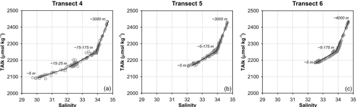
Figure 2.Total alkalinity versus salinity throughout the entire water column of sampling stations along transects 4(a), 5(b)and 6(c)off Oregon and northern California in spring/early summer 2007. The solid lines indicate various linear relationships observed on each transect. The numbers in italics denote the sampling depth/depth range of the endpoints of each line.
2 Study area and data source
2.1 California Current system and upwelling circulation
The upwelling circulation off Oregon and northern Califor-nia is linked with the eastern boundary current, the CaliforCalifor-nia Current (CC), occupying the open basin of the eNP (Barth et al., 2000). The CC is a broad and weak surface current (0–200 m) which carries low-salinity/low-temperature water equatorward from the sub-Arctic Pacific (Lynn and Simp-son, 1987). The deeper-lying California Undercurrent (CUC, 150–300 m), which has relatively high salinity and temper-ature, originates in the eastern equatorial Pacific and flows poleward inshore along the west coast of North America (Thomson and Krassovski, 2010). The CC system is charac-terized by coastal upwelling in spring/summer, during which waters primarily composed of the CC are transported upward from the depths of 150–200 m towards the nearshore surface off the Oregon–California coast (Castro et al., 2001).
Both field observations and modeling studies (Oke et al., 2002; Gan and Allen, 2005) show that the upwelling circu-lation pattern in the study area differs significantly between north and south of Newport (Fig. 1). North of Newport be-tween 45.0 and 45.5◦N with a relatively straight coastline and narrow shelf, the alongshore uniform bottom topogra-phy generally results in typical upwelling circulation with a southward coastal jet close to shore at Cascade Head (Fig. 1). Over the central Oregon shelf between 43.5 and 45.0◦N, the highly variable bottom topography over Heceta Bank (Fig. 1) largely influences the upwelling circulation, leading to a complex three-dimensional flow pattern with offshore shifting of the coastal jet and development of northward flow inshore. At the coast along the southern part of Oregon and northern California between 39.0 and 43.0◦N, an
enhance-ment of coastal upwelling, jet separation and eddy formation are observed to be associated with interactions of the wind-forced coastal currents with Cape Blanco (Fig. 1) (Barth and Smith, 1998; Gan and Allen, 2005, and references therein).
2.2 Data source
Our data sets were based on the online-published car-bonate system and nutrient data collected along three transects off Oregon and northern California during the first North American Carbon Program (NACP) West Coast Cruise in spring/early summer (11 May–14 June) 2007 (http://cdiac.ornl.gov/oceans/Coastal/NACP_West.html; Feely et al., 2008; Feely and Sabine, 2011). Transect 4 (stations 25–33 from nearshore to offshore) is located off Newport, Oregon. Transect 5 (stations 41–35 from nearshore to offshore) is located off Crescent City near the Oregon–California border. Transects 6 (stations 42–49 from nearshore to offshore) is located off Cape Mendocino, California. The majority of the offshore stations on all transects were located in the open subtropical gyre of the eNP (Fig. 1).
3 Results and discussion
The region under study is highly dynamic, potentially in-volving coastal upwelling, the CR plume and pelagic waters mixed by various Pacific water masses (Hill and Wheeler, 2002). Instead of accounting for all of the water masses con-tributing to the CC system, the mixing scheme in the upper waters along the three transects was examined via the total alkalinity–salinity (TAlk–Sal) relationship obtained during the sampling period so as to quantify the conservative por-tion of DIC and nitrate (NO3). The end members were
there-fore identified under this relationship, which might have ex-perienced physical or biological alterations from their origi-nal water masses such as the CR and the CC. Subsequently, the biologically consumed DIC and NO3were quantified as
the difference between their conservative values predicted from the derived end-member mixing and the corresponding field measurements. Finally, the CO2 source/sink nature of
and NO3, and a simple sensitivity analysis was performed to
test the robustness of the approach.
3.1 TAlk–Sal relationship
3.1.1 Throughout the entire water column off Oregon and northern California
Three generally linear relationships between TAlk and salin-ity were observed throughout the entire water column along transect 4 (Fig. 2a). The first one was for waters with salinity lower than∼32.0 (corresponding to a depth of∼15–25 m),
which were significantly influenced by the CR plume. The second one was for waters composed primarily of the CC with salinity between ∼32.0 and ∼33.9, including those immediately below the surface buoyant layer at stations 26–32 and the surface waters at the outermost station 33 (Fig. 1). The higher-end salinity value of ∼33.9
corre-sponded to a depth range of ∼75–175 m, composed
pos-sibly of the upwelled high-salinity CUC waters. At station 27 (water depth ∼170 m) for instance, salinity at depths
of ∼130 and ∼160 m reached∼34.0 with TAlk values of ∼2260 µmol kg−1, which were even higher than those of
off-shore waters at∼175 m (∼2250 µmol kg−1). These two data
points were thus located on the third linear relationship for waters with salinity higher than ∼33.9, the slope of which
became much steeper, mainly reflecting the mixing between the approaching CUC and deep waters in the subtropical gyre of the eNP (Fig. 2a).
All salinity values, including surface samples on transects 5 and 6, were higher than 32.0 (Fig. 2b and c). With minor influence of the CR plume, the TAlk–Sal relationship dis-played two generally linear phases throughout the entire wa-ter column along both transects, while the TAlk and salinity endpoints of each were comparable to those of the latter two observed on transect 4 (i.e., the linear phases for waters with salinity between∼32.0 and∼33.9 and with salinity higher
than∼33.9; Fig. 2a). Note that the turning point with salinity
of∼33.9 corresponded to a wider depth range of∼5–175 m
(Fig. 2b and c), resulting from the most intensive upwelling on transects 5 and 6 bringing deep waters to the nearshore surface (Feely et al., 2008).
As suggested by the generally linear TAlk–Sal relation-ships, surface waters beyond the CR plume and waters imme-diately below the surface buoyant layer were directly linked to the underlying waters to the depth of ∼175 m. We thus took a closer look at the TAlk–Sal relationship in the upper 175 m waters off Oregon and northern California.
3.1.2 In the upper 175 m waters off Oregon and northern California
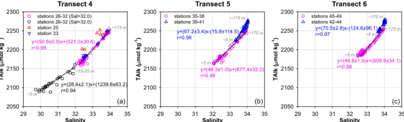
In the upper 175 m waters along transect 4, the linear re-gression for waters with salinity lower than ∼32.0 had an
intercept of∼1200 µmol kg−1. This value agreed well with
the observed TAlk of∼1000 µmol kg−1 in the mainstream
of the CR (Park et al., 1969b; Evans et al., 2013). The other linear regression for waters with salinity between∼32.0 and
∼33.9 had a smaller intercept of∼500 µmol kg−1, implying a smaller contribution from the CR plume (Fig. 3a). Excep-tions were observed at the shallowest station 25 (water depth
∼50 m) and the deepest station 33 (water depth∼2900 m).
The TAlk–Sal relationship completely followed the second phase for the upper 175 m waters at station 33 (Fig. 3a), sug-gesting a small fraction of the CR plume even in the surface waters of this outermost station on transect 4. On the other hand, data points of the two variables were not well corre-lated throughout the entire water column of station 25 and fell off both regression lines (Fig. 3a). The water mass mix-ing at this innermost station was not as straightforward, de-spite minor freshwater admixture as suggested by the high surface salinity of > 32.0.
The TAlk–Sal relationship in the upper 175 m waters on transects 5 and 6 displayed two similar phases. One was the linear regression for stations 35–38 (deeper than∼800 m)
and stations 45–49 (deeper than∼1400 m), with slope and
intercept values comparable to the second phase observed on transect 4. The other was the linear regression for the three shallow stations on both transects largely influenced by coastal upwelling (Feely et al., 2008) (Fig. 3b and c). This phase was not clearly seen from the full TAlk–Sal plot (Fig. 2b and c), as the salinity in the upper 175 m waters at stations 39 and 44 as well as in the entire water col-umn of stations 40–43 varied within a much smaller range of∼33.3–∼34.0. The negligible intercepts of this TAlk–Sal regression suggested insignificant freshwater input with zero solutes to the intensive upwelling zone off Oregon and north-ern California (Fig. 3b and c).
All phases shown in Fig. 3 displayed good linear TAlk–Sal relationships (r> 0.94), indicating an overall two-end-member mixing scheme for each phase. Although the non-conservativity of TAlk existed, it was not that signifi-cant as seen by the deviations of a few data points from each linear regression (Fig. 3). As a matter of fact, Fassbender et al. (2011) estimated that the contribution from CaCO3
dis-solution to the TAlk addition in the surface mixed layer on transect 5 was < 10 µmol kg−1(< 0.5 % of their absolute con-tents in seawater) and well near the analytical precision. Such small non-conservative portions would not compromise the application of TAlk as a conservative tracer. Note that the two-end-member mixing was not spatially homogeneous in the upper waters off Oregon and northern California during the sampling period. The surface waters at stations 26–32 on transect 4 were imprinted by the CR plume with a salin-ity around∼30.0. During the transport from the mouth of
Salinity
29 30 31 32 33 34 35
TAlk (
mol k
g
-1)
2050 2100 2150 2200 2250 2300
stations 26-32 (Sal>32.0) stations 26-32 (Sal<32.0) station 25
station 33
(a)
Salinity
29 30 31 32 33 34 35
TAlk (
mol k
g
-1)
2050 2100 2150 2200 2250 2300
stations 35-38 stations 39-41
(b)
Salinity
29 30 31 32 33 34 35
TAlk (
mol k
g
-1)
2050 2100 2150 2200 2250 2300
stations 45-49 stations 42-44
(c) y=(46.3±1.0)x+(677.4±32.2)
r=0.99 y=(67.2±3.4)x-(15.8±114.5) r=0.96
y=(28.4±2.1)x+(1239.8±63.2) r=0.94
y=(50.9±0.9)x+(521.0±30.6) r=0.99
Transect 4 Transect 5
~15-25 m ~175 m
~175 m ~175 m
~5 m
~5 m
~5 m
Transect 6
y=(46.8±1.0)x+(609.9±34.1) r=0.98
y=(70.5±2.8)x-(124.6±96.1) r=0.97
~175 m ~175 m
~5 m
~5 m
Figure 3.Total alkalinity versus salinity (TAlk–Sal relationship) in the upper 175 m waters of sampling stations along transects 4(a), 5(b) and 6(c)off Oregon and northern California in spring/early summer 2007. The solid lines as well as the equations (in accordance with the symbol colors) indicate the linear regression analyses of the TAlk–Sal relationship for various stations. The numbers in italics denote the sampling depth/depth range of the endpoints of each line. In(a), the TAlk–Sal relationship at station 26–32 displayed two phases for waters with salinities lower and higher than∼32.0. The surface waters at these stations were imprinted by the Columbia River plume. The data points of bottom waters at stations 26 (∼75 m) and 27 (∼130 and∼160 m) were not included, as they were located on the third linear relationship shown in Fig. 2a. In(b)and(c), stations 39–41 and stations 42–44 were largely influenced by coastal upwelling.
waters, brought up through coastal upwelling and/or verti-cal mixing. The influence of the CR plume still occurred but was diluted by other freshwater masses such as rainwater, suggesting a mixing scheme between the deep water in the subtropical gyre of the eNP and a combined freshwater end member (Park, 1966, 1968). Such mixing was also applica-ble to the surface waters at stations 35–38 on transect 5 and stations 45–49 on transect 6. On the other hand, the upper 175 m waters or the entire water column at stations 39–44 resulted from a simple two-end-member mixing between the upwelling source water and the rainwater with zero solutes, pointing to an apparent OceMar-type system.
3.2 1DIC and 1NO3 in the upper waters off Oregon and northern California
The defined mixing schemes enabled us to estimate the non-conservative portion of DIC (1DIC) and NO3(1NO3)in the
upper waters off Oregon and northern California following Dai et al. (2013):
1DIC=DICcons−DICmeas, (1)
1NO3 =NOcons3 −NO meas
3 , (2)
Xcons=Sal meas
Salref
·(Xref−Xeff)+Xeff. (3)
The superscripts “cons” and “meas” in Eqs. (1) and (2) de-note conservative-mixing-induced and field-measured val-ues. In Eq. (3), X represents DIC or NO3, while Salmeas
is the Conductivity–Temperature–Depth (CTD) recorder-measured salinity. Salref andXref are the reference salinity
and concentration of DIC or NO3 for the deep water end
member, which are the averages of all∼175 m samples from stations involved in each mixing scheme. Specifically, for waters immediately below the surface buoyant layer at tions 27–32 and waters in the surface mixed layer at sta-tions 25 and 33 on transect 4, the deep water end-member values of the reference salinity and concentrations of DIC or NO3were the averages of∼175 m samples from stations
28–33 (Fig. 1). On transects 5 and 6, the preformed salinity, DIC and NO3 values for waters in the surface mixed layer
at stations 35–38 and at stations 45–49 were the averages of
∼175 m samples of these stations. For the upper waters
in-fluenced by the intensified upwelling at stations 39–41 and stations 42–44, the deep water end member was selected as the∼175 m water at station 39 and at station 44 (Fig. 1).
The Xeff in Eq. (3) denotes the effective concentration of DIC or NO3 sourced from the freshwater input to
vari-ous zones off Oregon and northern California. Since rainwa-ter was assumed to have no solutes, both DICeff and NOeff3 would be zero for waters in the surface mixed layer of sta-tions 39–41 on transect 5 and stasta-tions 42–44 on transect 6. On the other hand, the estimation ofXeffassociated with the CR followed the method for the OceMar case study of the CS, which has a noticeable DICeff from the combination of the Amazon River and the Orinoco River (Dai et al., 2013).
Since bicarbonate dominates other CO2species and other
alkalinity components, DIC concentrations in the main-stream of the CR are numerically similar to TAlk, which are also around∼1000 µmol kg−1(Park et al., 1969a, 1970).
This value was taken as the DIC end member of the CR. The NO3 end-member value was selected as 15 µmol kg−1
http://www.stccmop.org/datamart/). Assuming that the bio-logical consumption of DIC and NO3in the CR plume
fol-lowed the Redfield ratio (Redfield et al., 1963), the DIC re-moval was estimated to be∼100 µmol kg−1(approximately 15×106/16), while NO3 was rapidly consumed along the
pathway of the CR plume and generally depleted in the area beyond the plume (Aguilar-Islas and Bruland, 2006; Lohan and Bruland, 2006). As a consequence, the complete DICeff and NOeff3 in the upper waters from the CR would be∼900
and∼0 µmol kg−1.
If the combined freshwater end member was a mixture of the CR and the rainwater with zero solutes, the inter-cept values of 521.0±30.6 (Fig. 3a), 677.4±32.2 (Fig. 3b) and 609.9±34.1 (Fig. 3c) derived from the TAlk–Sal re-gression would indicate that the CR fractions were ∼50,
∼65 and∼60 % (approximately 500/1000, 650/1000 and
600/1000 taking∼1000 µmol kg−1as the TAlk end-member
value of the CR, Park et al., 1969b; Evans et al., 2013). The DICeff from the freshwater input was thus estimated to be ∼450 µmol kg−1(approximately 900×50 %) for
wa-ters immediately below the surface buoyant layer at tions 27–32 and waters in the surface mixed layer at sta-tions 25 and 33 on transect 4, which was slightly lower than the ∼585 µmol kg−1 (approximately 900×65 %) and
the∼540 µmol kg−1(approximately 900×60 %) for waters
in the surface mixed layer at stations 35–38 on transect 5 and at stations 45–49 on transect 6, respectively. The NOeff3 in any combined freshwater end member was zero.
Note that numerous small mountain rivers are distributed along the Oregon–California coast, which might also dilute the CR plume, inducing the lower intercept of the TAlk–Sal regression observed on the three transects (Fig. 3). The av-erage wintertime discharge from the Oregon Coast Range rivers is estimated to be∼2570 m3s−1(Wetz et al., 2006),
which is more than an order of magnitude higher than that in the summer (Colbert and McManus, 2003; Sigleo and Frick, 2003). However, the CR discharge in May to June 2007 reached its maximum of∼15 000 m3s−1(Evans et al.,
2013), which should be approximately 2 orders of magni-tude higher than the discharge of small rivers. This significant contrast would suggest that inputs from small rivers should be negligible compared to the CR plume. In particular, inputs from small rivers are normally restricted to a narrow band near the coast, whereas the research domain of this study extended to the open subtropical gyre of the eNP. Even the surface salinity at the innermost stations (i.e., station 25 on transect 4, station 41 on transect 5 and station 42 on transect 6; Fig. 1) was as high as∼32.5,∼33.9 and∼34.0, which
would rule out the influence of small rivers.
3.3 Evaluating the CO2source/sink nature in the upper waters off Oregon and northern California
The coupling of DIC and NO3 dynamics could then
be examined based on the classic Redfield ratio of
C : N=106 : 16=6.6 (Redfield et al., 1963). Positive val-ues of the difference between 1DIC and 6.61NO3
(1DIC−6.61NO3)suggested a CO2source term since
“ex-cess 1DIC” was removed by CO2 degassing into the
at-mosphere. In contrast, negative1DIC−6.61NO3suggested
that “deficient1DIC” was supplied via the atmospheric CO2
input to the ocean, representing a CO2sink. Such net CO2
ex-change between the seawater and the atmosphere was further quantified as the sea–air difference ofpCO2(1pCO2)via
the Revelle factor (RF), which is referred to as the fractional change in seawater CO2over that of DIC at a given
temper-ature, salinity and alkalinity, and indicates the ocean’s sensi-tivity to an increase in atmospheric CO2(Revelle and Suess,
1957; Sundquist et al., 1979). BecausepCO2 and CO2 are
proportional to each other, the RF can be illustrated as: RF= ∂pCO2/ pCO2
∂DIC/DIC . (4)
Here,∂pCO2and∂DIC are the fractional changes ofpCO2
and DIC in the surface seawater. In a simplified way and as an approximation,∂DIC equals1DIC−6.61NO3, which is
solely achieved through sea–air CO2 exchange in the
Oce-Mar framework, implying that ∂pCO2 may represent the
sea–air1pCO2. Given an initial balance of CO2between the
seawater and the atmosphere, the sea–air1pCO2is obtained
by
Sea–air1pCO2=∂pCO2=RF·pCO2·
∂DIC
DIC (5)
=RF·pCOair 2 ·
1DIC−6.61NO3
DIC .
As shown in Fig. 4, the estimated1DIC−6.61NO3values
and their corresponding sea–air1pCO2values in the upper
waters off Oregon and northern California were overall be-low zero, suggesting a significant CO2sink nature in the
up-welling season.
3.3.1 Transect 4
On transect 4 off Newport, the average value of 1DIC−6.61NO3 was −23±2 µmol kg−1 in waters
immediately below the surface buoyant layer at stations 27–32, which equaled the average value for the surface mixed layer at station 33 (Fig. 4a). Note that we were not able to derive values of 1DIC−6.61NO3 at station 26
where NO3 data were not available. Although located at
different depths, the two water parcels experienced similar physical mixing and biogeochemical modifications inducing the same CO2signature. The former water mass should work
as a CO2sink when in contact with the atmosphere before
or after the passage of the episodic CR plume. The average sea–air1pCO2resulting from the combined deficient1DIC
was−54±4 µatm (Fig. 3a). Given the atmosphericpCO2of ∼390 µatm (Evans et al., 2011), the seawaterpCO2in these
Salinity
31.5 32.0 32.5 33.0 33.5 34.0 34.5
DI C-6 .6 NO 3 ( mo l kg -1) -70 -60 -50 -40 -30 -20 -10 0 10 Sea -ai
r
p CO 2 ( atm) -70 -60 -50 -40 -30 -20 -10 0 10 stations 27-32 station 33 Salinity
31.5 32.0 32.5 33.0 33.5 34.0 34.5
DIC-6.6 NO 3 ( mo l kg -1) -70 -60 -50 -40 -30 -20 -10 0 10 Sea-air p CO 2 ( at m) -70 -60 -50 -40 -30 -20 -10 0 10 stations 35-38 stations 39-41 (a) (b) Salinity
31.5 32.0 32.5 33.0 33.5 34.0 34.5
DIC-6.6 NO 3 ( mo l kg -1) -70 -60 -50 -40 -30 -20 -10 0 10 Sea-air p CO 2 ( at m) -70 -60 -50 -40 -30 -20 -10 0 10 stations 45-49 stations 42-44 (c)
Transect 4 Transect 5 Transect 6
Figure 4.1DIC−6.61NO3(squares) and sea–air1pCO2(triangles) versus salinity in the upper waters on transects 4(a), 5(b)and 6(c)off
Oregon and northern California in spring/early summer 2007. Note that data for stations 27–32 on transect 4 were obtained from waters immediately below the surface buoyant layer, while data for other stations were obtained from the surface mixed layer. The value of 6.6 is the Redfield C / N uptake ratio (approximately 106/16; Redfield et al., 1963). The solid line indicates thepCO2equilibrium between the
seawater and the atmosphere.
rather well with the field measurements of 334±13 µatm (the underway seawaterpCO2data were not available online
but alternatively calculated by applying TAlk and DIC data to the CO2SYS program; Lewis and Wallace, 1998).
The diagnostic approach was not applied to the surface buoyant layer since the aged CR plume might have ex-perienced complex mixing with various surrounding wa-ter masses during its transport, as indicated by the scat-ter TAlk–Sal relationship (Fig. 3a). However, the far-field CR plume is suggested to be a strong sink of atmospheric CO2 due to earlier biological consumption (Evans et al.,
2011), which was supported by the observed low pCO2of ∼220–300 µatm in the surface buoyant layer on transect 4.
As a consequence, the CO2 sink nature in the upper
wa-ters from the outer shelf (the bottom depth of station 27 was
∼170 m) to the open basin off Newport, Oregon would pri-marily result from the higher utilization of nutrients relative to DIC based on their concurrent inputs from deep waters. The non-local high productivity in the CR plume could in-ject even lowerpCO2, but this effect would be transitory.
At the innermost station 25 on transect 4, highly pos-itive values of 1DIC−6.61NO3 and sea–air 1pCO2
(∼82 µmol kg−1 and ∼157 µatm, respectively) were
ob-tained for the surface mixed layer of this station, indicating a significant CO2source. However, the lowestpCO2value of ∼170 µatm was observed in these nearshore waters off
Ore-gon. The poor correlation between TAlk and salinity at sta-tion 25 (Fig. 3a) might compromise the estimasta-tion, whereas the same method (Eqs. 1–5) was successfully applied to other stations on transect 4 with a distinct TAlk–Sal relationship (i.e., the second phase in Fig. 3a). Note that coastal upwelling clearly influenced the bottom water at station 25 as indicated by the comparable salinity and TAlk values to those in off-shore 200 m waters. Instead of being fed by the upwelled deep water, the DIC and nutrients in the surface mixed layer might have originated from horizontal admixture of the sur-rounding waters. These waters possibly experienced intense
diatom blooms due to the fact that the surface silicate con-centrations at station 25 were almost zero, which led to the most undersaturatedpCO2condition observed in the upper
waters off Oregon.
3.3.2 Transects 5 and 6
On transect 5 near the Oregon–California border, the average 1DIC−6.61NO3and sea–air1pCO2were estimated to be −20±3 µmol kg−1and−48±8 µatm in the surface mixed
layer of stations 35–38 (Fig. 4b). Both values were compara-ble to those obtained from the surface mixed layer of stations 45–49 on transect 6 (−23±3 µmol kg−1and−53±6 µatm,
respectively; Fig. 4c) and on transect 4, indicating a similar magnitude of the CO2sink term in offshore areas along the
Oregon and northern California coast during the sampling period. The estimated sea surfacepCO2of 342±8 µatm for
transect 5 and 337±6 µatm for transect 6 were consistent
with the field measurements of 332±12 and 346±12 µatm
in these regions.
The diagnosed CO2flux in the nearshore was also
com-parable between transects 5 and 6. The 1DIC−6.61NO3
and sea–air1pCO2 in the surface mixed layer of stations
39–44, although still below zero, were obviously higher than those of stations 35–38 on transect 5 and of stations 45–49 on transect 6 (Fig. 4b and c). Such an increase was ex-pected since stations 39–44 were located in the area with the most intensive upwelling, which brought CO2-rich deep
wa-ters to the nearshore surface (Feely et al., 2008). However, our estimation suggested a weaker CO2sink or close to
be-ing in equilibrium with the combined estimated sea surface pCO2of 368±14 µatm, whereas the field measurements of ∼600–1000 µatm indicated that the coastal upwelling zone
should be a very strong source of CO2to the atmosphere.
Therefore, we took a closer look at transect 5: a uni-form salinity of∼34.0 throughout the entire water column
on transect 5 (Feely et al., 2008). Although salinity in the surface mixed layer at station 39 was lower, around∼33.4, the dilution effect of rainwater should be negligible. After removing the rainwater from the mixing scheme and cal-culating1DIC and1NO3 by directly subtracting the
field-observed value from the end-member value for the upwelling source water (Eqs. 6 and 7; DICref and NOref3 were field measurements of∼200 m water samples at station 39), the
1DIC−6.61NO3 values were rapidly increased to above
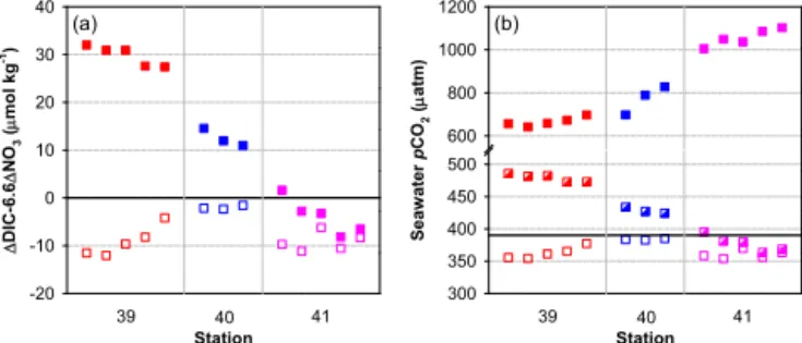
zero in the surface mixed layer at stations 39 and 40, while values at station 41 with a small increase were still over-all below zero (Fig. 5a). Correspondingly, the estimated sea surfacepCO2values were higher than the atmospheric CO2
value at stations 39 and 40 while they were slightly lower than that at station 41. However, these values still largely fell below the field measurements of seawaterpCO2, displaying
shoreward increasing differences from∼200 to∼700 µatm (Fig. 5b).
1DIC=DICref−DICmeas, (6)
1NO3 =NOref3 −NOmeas3 . (7)
With or without taking rainwater into account, our diagnos-tic approach did not work in the nearshore areas with strong upwelling off Oregon and northern California, even though the mixing scheme of this region was in accordance with the OceMar concept. We contend that OceMar assumes a steady state with balanced DIC and nutrients via both physical mixing and biological alterations in comparable timescales. However, the continuous inputs from the coastal upwelling might have led to the accumulation of DIC and nutrients in the nearshore surface, which could not be timely consumed by the phytoplankton community, suggesting a possible non-steady state. Fassbender et al. (2011) estimated that the age of the surface mixed layer at nearshore stations on transect 5 is only∼0.2 days, during which the DIC and NO3
con-sumption via organic carbon production was almost zero, and CaCO3dissolution contributed a small fraction to the slightly
elevated DIC in the upwelled waters. They further predicted that the nearshore surfacepCO2on transect 5 will decrease
to levels of∼200 µatm in∼30 days until NO3exhaustion
via continued biological productivity, implying the achieve-ment of a steady state (Fassbender et al., 2011). Minor bi-ological responses during the intensified upwelling period were also observed in summer 2008, allowing highly over-saturated pCO2 surface water to persist on the inner shelf
off Oregon for nearly 2 months (Evans et al., 2011). At this point, it is uncertain why there was such a prolonged delay from the phytoplankton community to the persistent source of upwelled DIC and nutrients. Note that under the condition of a more prevailing upwelling-favorable wind as a predicted consequence of climate change (e.g., Snyder et al., 2003; Dif-fenbaugh et al., 2004; Sydeman et al., 2014), the nearshore
Station
DIC
-6.6
NO
3
(
mol kg
-1)
-20 -10 0 10 20 30 40
39 40 41
(a)
Station
Seaw
ater
p
CO
2
(
atm)
300 350 400 450 500 600 800 1000 1200
39 40 41
(b)
Figure 5.Panel(a)shows1DIC−6.61NO3and(b)shows
seawa-terpCO2in the surface mixed layer at stations 39–41 on transect
5 near the Oregon–California border in spring/early summer 2007. In(a), open symbols indicate values estimated based on the two-end-member mixing between the upwelling source water and the rainwater, while filled symbols indicate values after removing the rainwater. The value of 6.6 is the Redfield C / N uptake ratio (ap-proximately 106/16; Redfield et al., 1963). The solid line indicates thepCO2 equilibrium between the seawater and the atmosphere.
In(b), the open and semi-filled symbols denote the estimated sea surfacepCO2from1DIC−6.61NO3on top of the mixing with
and without rainwater, respectively. The filled symbols denote the field-observed sea surfacepCO2, which were obtained by applying
TAlk and DIC data into the CO2SYS program (Lewis and Wallace, 1998). The solid line denotes the atmosphericpCO2of∼390 µatm
(Evans et al., 2011).
waters off the Oregon–California coast in the upwelling sea-son might always be in a non-steady state, and it is expected that fewer periodic relaxation events or reversals would fur-ther decrease the chance for the biological response to be factored in.
In addition, the negligible biological consumption might involve large errors when calculating 1. The portion of 1DIC and 1NO3 at station 41 relative to the preformed
values of the upwelling source water were only∼0.5 and ∼10 %, slightly higher than the measurement uncertainties.
The portion of DIC and NO3 consumption in the surface
mixed layer at offshore stations on transect 5 were, how-ever, 1 order of magnitude higher (∼7 and∼90 %,
respec-tively). This contrast might partially explain why the Oce-Mar framework did not work when insignificant biological alterations occurred. Given the predominant control of phys-ical mixing, we contend that the prediction of the CO2flux
in the nearshore off Oregon and northern California with intensified upwelling could be simplified without consider-ing DIC/nutrient consumption. In other words, surface CO2
levels in this region were simply imprints of the upwelling source water (pCO2∼1000 µatm at∼150–200 m) with
mi-nor dilution by rainwater.
3.4 Sensitivity analysis
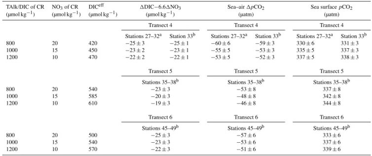
Table 1.Values of1DIC−6.61NO3, sea–air1pCO2and sea surfacepCO2estimated with different DICeff, which is the combined
fresh-water end member of DIC partly sourced from the Columbia River (CR).
TAlk/DIC of CR NO3of CR DICeff 1DIC−6.61NO3 Sea–air1pCO2 Sea surfacepCO2
(µmol kg−1) (µmol kg−1) (µmol kg−1) (µmol kg−1) (µatm) (µatm)
Transect 4 Transect 4 Transect 4
Stations 27–32a Station 33b Stations 27–32a Station 33b Stations 27–32a Station 33b
800 20 420 −25±3 −25±1 −60±6 −59±3 330±6 331±3
1000 15 450 −23±2 −23±1 −55±5 −53±3 335±5 337±3
1200 10 470 −22±2 −22±1 −53±5 −52±3 337±5 338±3
Transect 5 Transect 5 Transect 5
Stations 35–38b Stations 35–38b Stations 35–38b
800 20 540 −23±3 −53±8 337±8
1000 15 585 −20±3 −48±8 342±8
1200 10 610 −19±3 −46±8 344±8
Transect 6 Transect 6 Transect 6
Stations 45–49b Stations 45–49b Stations 45–49b
800 20 500 −25±3 −57±6 333±6
1000 15 540 −23±3 −53±6 337±6
1200 10 570 −22±3 −51±6 339±6
aData for these stations were obtained from waters immediately below the surface buoyant layer.bData for these stations were obtained from the surface mixed layer.
Table 2. Values of1DIC−6.61NO3, sea–air1pCO2and sea surfacepCO2estimated with the deep water end member from different depths.
Depth of the deep 1DIC−6.61NO3 Sea–air1pCO2 Sea surfacepCO2
water end member (m) (µmol kg−1) (µatm) (µatm)
Transect 4 Transect 4 Transect 4
Stations 27–32a Station 33b Stations 27–32a Station 33b Stations 27–32a Station 33b
∼130 −23±2 −19±1 −56±5 −45±3 334±5 345±3
∼150 −23±2 −22±1 −55±5 −52±3 335±5 338±3
∼175 −23±2 −23±1 −55±5 −53±3 335±5 337±3
∼200 −23±2 −24±1 −55±5 −56±3 335±5 334±3
Transect 5 Transect 5 Transect 5
Stations 35–38b Stations 35–38b Stations 35–38b
∼130 −21±3 −51±8 339±8
∼150 −20±3 −46±8 344±8
∼175 −20±3 −48±8 342±8
∼200 −17±3 −40±8 350±8
Transect 6 Transect 6 Transect 6
Stations 45–49b Stations 45–49b Stations 45–49b
∼130 −20±3 −46±6 344±6
∼150 −22±3 −51±6 339±6
∼175 −23±3 −53±6 337±6
∼200 −21±3 −50±6 340±6
important in resolving the CO2fluxes. We thus conducted a
sensitivity analysis for these two sets of variables for the CO2
sink zones off Oregon and northern California where our di-agnostic approach worked well (i.e., waters immediately be-low the surface buoyant layer at stations 27–32 as well as waters in the surface mixed layer at station 33 on transect 4, waters in the surface mixed layer at stations 35–38 on tran-sect 5 and waters in the surface mixed layer at stations 45–49 on transect 6).
3.4.1 The combined freshwater end member
While the values of ∼1000 and ∼15 µmol kg−1 were
se-lected for TAlk/DIC and NO3in the mainstream of the CR,
the field-observed TAlk and NO3 vary within a range of ∼800–1200 (Evans et al., 2013) and ∼10–20 µmol kg−1
(http://www.stccmop.org/datamart/) in spring/early summer. We thus took the values of∼800 and∼1200 µmol kg−1as
the lower and upper limit of the TAlk and DIC end mem-bers and those of∼10 and∼20 µmol kg−1as the lower and
upper limit of the NO3 end member in the CR to test the
diagnostic approach. Following the same calculation of the combined freshwater end member (Xeffin Eq. 3), the lower and upper limit of DICeff was estimated to be ∼420 and ∼470 µmol kg−1for waters immediately below the surface
buoyant layer at stations 27–32 and in the surface mixed layer at station 33 on transect 4. Those values were∼540
and∼610 µmol kg−1for waters in the surface mixed layer at
stations 35–38 on transect 5, and∼500 and∼570 µmol kg−1
in the surface mixed layer at stations 45–49 on transect 6. The NOeff3 in every scenario was still zero.
The newly diagnosed 1DIC−6.61NO3 and sea–air
1pCO2on transects 4, 5 and 6 displayed no difference with
those with the initial TAlk and DIC of∼1000 µmol kg−1and
NO3of ∼15 µmol kg−1in the CR (Table 1), while all
esti-mated sea surfacepCO2values were within error (1 standard
deviation) compared to the field measurements. Although the TAlk and DIC end members had large variations of up to
∼400 µmol kg−1while NO3 varied within∼10 µmol kg−1
in the mainstream of the CR, the corresponding range of DICeff contributing to waters beyond the CR plume signif-icantly decreased by approximately 1 order of magnitude, implying minor influence of its variations on our diagnosis of the CO2fluxes.
3.4.2 The deep water end member
We selected values at∼175 m as the deep water end mem-ber based on the TAlk–Sal relationship, whereas this end member depth might not be spatially stable in a highly dy-namic upwelling system. Previous studies also show that the upwelling source water on the Oregon–California shelf can vary between 150 and 200 m (e.g., Hales et al., 2005; Feely et al., 2008). We thus tested the diagnostic approach with values at three other depths of∼130,∼150 and∼200 m.
On transects 4 and 6, the newly estimated 1DIC−6.61NO3, sea–air 1pCO2 and sea surface pCO2
using end-member values at both∼150 and∼200 m agreed well with those using end-member values at∼175 m, while the three variables were slightly higher using end-member values at ∼130 m (Table 2). On transect 5, the newly
estimated 1DIC−6.61NO3, sea–air 1pCO2 and sea
sur-face pCO2 using end-member values at both ∼130 and ∼150 m agreed well with those using end-member values at ∼175 m, while the three variables were slightly higher using
end-member values at∼200 m (Table 2).
3.4.3 The C / N uptake ratio
In a given oceanic setting, the real C / N uptake ratio during organic carbon production can be different from the Redfield stoichiometry of∼6.6 (Redfield et al., 1963). For instance, higher ratios estimated from the DIC–NO3relationship are
observed in both coastal waters and open ocean sites, pos-sibly resulting from excess DIC uptake via the production of dissolved organic carbon (Sambrotto et al., 1993; Ianson et al., 2003). However, since the precise estimation of the C / N uptake ratio (via, for example, in situ incubation ex-periments) is still problematic, such data are currently scarce over the world’s oceans, and the empirical stoichiometry is routinely applied into field studies investigating the dynam-ics and coupling of carbon and nutrients (e.g., Chen et al., 2008; Fassbender et al., 2011). Fassbender et al. (2011) ap-plied another empirical C / N uptake ratio of 7.3 (approxi-mately 117/16; Anderson and Sarmiento, 1994) into the same data set as this study. We thus performed a simple sensitiv-ity analysis using this alternative value of 7.3, which implies excess DIC uptake relative to NO3.
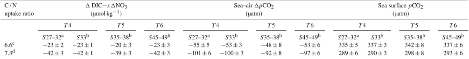
Since 1DIC−7.31NO3 values were obviously smaller
than1DIC−6.61NO3 ones, the new sea–air 1pCO2
val-ues were halved (Table 3). Correspondingly, the newly esti-mated sea surfacepCO2values on transects 4, 5 and 6 were ∼35–45 µatm lower than the estimation using the Redfield
ratio, which were however consistent with the field mea-surements. Given that the Redfield ratio also works in our OceMar case studies of the SCS and the CS (Dai et al., 2013), we contend that this classic ratio could be preferen-tially employed if the field-observed elemental stoichiometry is not available. Moreover, as Martz et al. (2014) pointed out, “treating the Redfield ratios as global or regional constants may be acceptable in the context of interpreting snapshots of the water column captured in shipboard bottle data”.
The above notion was also supported by examining the slope of the linear regression between DIC and NO3
Table 3.Values of sea–air1pCO2and sea surfacepCO2estimated with different1DIC−x1NO3. The variablexdenotes the C / N uptake
ratio during organic carbon production.T andSrepresent transect and station(s).
C / N 1DIC−x1NO3 Sea–air1pCO2 Sea surfacepCO2
uptake ratio (µmol kg−1) (µatm) (µatm)
T4 T5 T6 T4 T5 T6 T4 T5 T6
S27–32a S33b S35–38b S45–49b S27–32a S33b S35–38b S45–49b S27–32a S33b S35–38b S45–49b
6.6c −23±2 −23±1 −20±3 −23±3 −55±5 −53±3 −48±8 −53±6 335±5 337±3 342±8 337±6
7.3d −42±3 −42±1 −39±3 −42±3 −101±6 −100±3 −92±8 −97±6 289±6 290±3 298±8 293±6
aData for these stations were obtained from waters immediately below the surface buoyant layer.bData for these stations were obtained from the surface mixed layer.
c6.6 is the Redfield C / N uptake ratio (approximately 106/16; Redfield et al., 1963).d7.3 is the more recent evaluation of the C / N uptake ratio (approximately 117/16;
Anderson and Sarmiento, 1994).
normalization (Friis et al., 2003; Cao et al., 2011) as:
nX=X
meas−Xeff
Salmeas ·Sal
aver+Xeff. (8)
Here, nX and Xmeas are salinity-normalized and field-measured values for DIC and NO3. Salmeas is the
CTD-measured salinity. Salaver is the average salinity value of
∼33.0 in these CO2sink zones, which was selected as the
constant salinity.Xeff is the same as that in Eq. (3), denot-ing the effective concentration of DIC or NO3sourced from
the freshwater input to various zones off Oregon and north-ern California. While the NOeff3 in any combined freshwa-ter end member was zero, the DICeff was∼450 µmol kg−1
for waters immediately below the surface buoyant layer at stations 27–32 and waters in the surface mixed layer at sta-tions 25 and 33 on transect 4, ∼585 µmol kg−1 for waters
in the surface mixed layer at stations 35–38 on transect 5, and∼540 µmol kg−1for waters in the surface mixed layer at
stations 45–49 on transect 6.
As shown in Fig. 6, our analysis with all data from the CO2 sink zones along the three transects revealed a slope
of 6.70±0.37. This value was within error comparable to
that of 6.6, suggesting that using the Redfield ratio in our diagnostic approach should be in order. On the other hand, we contend that scrutinizing the in situ C / N uptake ratio via relatively direct observations is imperative for better under-standing the issue regarding the possible departure from the Redfield ratio.
4 Concluding remarks
The semi-analytical diagnostic approach of mass balance that couples physical transport and biogeochemical alterations was well applied to the CO2sink zones off Oregon and
north-ern California in spring/early summer 2007, extending from the outer shelf to the open basin. In these zones with the absence of any significant influence of the CR plume, the source of DIC was largely from deep waters in the subtropi-cal gyre of the eNP, and the ultimate CO2sink nature was
de-termined by the higher nutrient consumption than DIC in the upper waters. On the other hand, the estimated CO2flux was
Figure 6. Salinity-normalized DIC (nDIC) versus salinity-normalized NO3 (nNO3)in the CO2 sink zones off Oregon and
northern California in spring/early summer 2007, which included waters immediately below the surface buoyant layer at stations 27–32 as well as waters in the surface mixed layer at station 33 on transect 4, waters in the surface mixed layer at stations 35–38 on transect 5 and waters in the surface mixed layer at stations 45–49 on transect 6.
opposite the field observations in the nearshore upwelling zone along the Oregon–California coast, which behaved like a typical OceMar system in terms of its mixing process. This discrepancy was very likely due to minor biological re-sponses during the intensified upwelling period, making our mass balance approach based on the coupled physical bio-geochemistry invalid. This suggested that the applicability of the proposed semi-analytical diagnostic approach is limited to steady state systems with comparable timescales of wa-ter mass mixing and biogeochemical reactions. In a physical mixing prevailing regime, resolving the CO2fluxes could
Acknowledgements. This work was funded by the National Key Scientific Research Project (no. 2015CB954000) and the National Basic Research Program (973) (no. 2009CB421200) sponsored by the Ministry of Science and Technology of the PRC. This work was also supported by the National Natural Science Foundation of China through grants 91328202, 41121091, 90711005 and 41130857. We are very grateful to the Carbon Dioxide Information Analysis Center (CDIAC; http://cdiac.ornl.gov/oceans/) for the online-published data of the first North American Carbon Program (NACP) West Coast Cruise. Z. Cao is supported by the Humboldt Research Fellowship for postdoctoral researchers provided by the Alexander von Humboldt Foundation. We thank John Hodgkiss for his help with the manuscript’s English. Comments from Rik Wanninkhof, Debby Ianson and another anonymous reviewer have significantly improved the quality of the paper.
Edited by: K. Fennel
References
Aguilar-Islas, A. M. and Bruland, K. W.: Dissolved manganese and silicic acid in the Columbia River plume: A major source to the California current and coastal waters off Washington and Ore-gon, Mar. Chem., 101, 233–247, 2006.
Allen, J. S., Newberger, P. A., and Federiuk, J.: Upwelling circula-tion on the Oregon continental shelf, Part I: Response to idealized forcing, J. Phys. Oceanogr., 25, 1843–1866, 1995.
Anderson, L. A. and Sarmiento, J. L.: Redfield ratios of rem-ineralization determined by nutrient data analysis, Global Bio-geochem. Cy., 8, 65–80, 1994.
Barth, J. A. and Smith, R. L.: Separation of a coastal upwelling jet at Cape Blanco, Oregon, USA, in: Benguela Dynamics: Impacts of Variability on Shelf-Sea Environments and their Living Re-sources, edited by: Pillar, S. C., Moloney, C. L., Payne, A. I. L., and Shillington, F. A., S. Afr. J. Mar. Sci., 19, 5–14, 1998. Barth, J. A., Pierce, S. D., and Smith, R. L.: A separating coastal
upwelling jet at Cape Blanco, Oregon and its connection to the California Current System, Deep-Sea Res. Pt. II, 47, 783–810, 2000.
Borges, A. V.: Present day carbon dioxide fluxes in the coastal ocean and possible feedbacks under global change, in: Oceans and the Atmospheric Carbon Content, edited by: Duarte, P. and Santana-Casiano, J. M., Springer Science+Business Media B.V., chap. 3, 47–77, 2011.
Borges, A. V. and Frankignoulle, M.: Distribution of surface car-bon dioxide and air-sea exchange in the upwelling system off the Galician coast, Global Biogeochem. Cy., 16, 13-1–13-13, doi:10.1029/2000GB001385, 2002.
Borges, A. V., Delille, B., and Frankignoulle, M.: Budget-ing sinks and sources of CO2 in the coastal ocean:
Diver-sity of ecosystems counts, Geophys. Res. Lett., 32, L14601, doi:10.1029/2005GL023053, 2005.
Cai, W.-J.: Estuarine and coastal ocean carbon paradox: CO2sinks
or sites of terrestrial carbon incineration?, Annu. Rev. Mar. Sci., 3, 123–145, 2011.
Cai, W.-J., Dai, M., and Wang, Y.: Air-sea exchange of carbon diox-ide in ocean margins: A province-based synthesis, Geophys. Res. Lett., 33, L12603, doi:10.1029/2006GL026219, 2006.
Cao, Z., Dai, M., Zheng, N., Wang, D., Li, Q., Zhai, W., Meng, F., and Gan, J.: Dynamics of the carbonate system in a large continental shelf system under the influence of both a river plume and coastal upwelling, J. Geophys. Res., 116, G02010, doi:10.1029/2010JG001596, 2011.
Castro, C. G., Chavez, F. P., and Collins, C. A.: Role of the Cal-ifornia Undercurrent in the export of denitrified waters from the eastern tropical North Pacific, Global Biogeochem. Cy., 15, 819–830, doi:10.1029/2000GB001324, 2001.
Chen, C.-T. A. and Borges, A. V.: Reconciling opposing views on carbon cycling in the coastal ocean: Continental shelves as sinks and near-shore ecosystems as sources of atmospheric CO2,
Deep-Sea Res. Pt. II, 56, 578–590, 2009.
Chen, F., Cai, W.-J., Wang, Y., Rii, Y. M., Bidigare, R. R., and Benitez-Nelson, C. R.: The carbon dioxide system and net com-munity production within a cyclonic eddy in the lee of Hawaii, Deep-Sea Res. Pt. II, 55, 1412–1425, 2008.
Colbert, D. and McManus, J.: Nutrient biogeochemistry in an upwelling-influenced estuary of the Pacific Northwest (Tillam-ook Bay, Oregon, USA), Estuaries, 26, 1205–1219, 2003. Dai, M., Cao, Z., Guo, X., Zhai, W., Liu, Z., Yin, Z., Xu, Y., Gan,
J., Hu, J., and Du, C.: Why are some marginal seas sources of atmospheric CO2?, Geophys. Res. Lett., 40, 2154–2158,
doi:10.1002/grl.50390, 2013.
Diffenbaugh, N. S., Snyder, M. A., and Sloan, L. C.: Could CO2-induced land-cover feedbacks alter near-shore upwelling regimes?, Proc. Natl. Acad. Sci. USA, 101, 27–32, 2004. Evans, W., Hales, B., and Strutton, P. G.: Seasonal cycle of surface
oceanpCO2on the Oregon shelf, J. Geophys. Res., 116, C05012,
doi:10.1029/2010JC006625, 2011.
Evans, W., Hales, B., Strutton, P. G., and Ianson, D.: Sea-air CO2
fluxes in the western Canadian coastal ocean, Prog. Oceanogr., 101, 78–91, 2012.
Evans, W., Hales, B., and Strutton, P. G.:pCO2distributions and
air-water CO2 fluxes in the Columbia River estuary, Estuar. Coast. Shelf Sci., 117, 260–272, 2013.
Fassbender, A. J., Sabine, C. L., Feely, R. A., Langdon, C., and Mordy, C. W.: Inorganic carbon dynamics during northern Cali-fornia coastal upwelling, Cont. Shelf Res., 31, 1180–1192, 2011. Federiuk, J. and Allen, J. S.: Upwelling circulation on the Oregon continental shelf. Part II: Simulations and comparisons with ob-servations, J. Phys. Oceanogr., 25, 1867–1889, 1995.
Feely, R. and Sabine, C.: Carbon dioxide and hydrographic measurements during the 2007 NACP West Coast Cruise, http: //cdiac.ornl.gov/ftp/oceans/NACP_West_Coast_Cruise_2007/, Carbon Dioxide Information Analysis Center, Oak Ridge National Laboratory, US Department of Energy, Oak Ridge, Tennessee, 2011.
Feely, R. A., Sabine, C. L., Hernandez-Ayon, J. M., Ianson, D., and Hales, B.: Evidence for upwelling of corrosive “acidified” water onto the continental shelf, Science, 320, 1490–1492, 2008. Fransson, A., Chierici, M., and Nojiri, Y.: Increased net CO2
Friis, K., Körtzinger, A., and Wallace, D. W. R.: The salinity nor-malization of marine inorganic carbon chemistry data, Geophys. Res. Lett., 30, 1085, doi:10.1029/2002GL015898, 2003. Gan, J. and Allen, J. S.: A modeling study of shelf circulation off
northern California in the region of the Coastal Ocean Dynam-ics Experiment, response to relaxation of upwelling, J. Geophys. Res., 107, 3123, doi:10.1029/2000JC000768, 2002.
Gan, J., and Allen, J. S.: Modeling upwelling circulation off the Oregon coast, J. Geophys. Res., 110, C10S07, doi:10.1029/2004JC002692, 2005.
Hales, B., Takahashi, T., and Bandstra, L.: Atmospheric CO2
up-take by a coastal upwelling system, Global Biogeochem. Cy., 19, GB1009, doi:10.1029/2004GB002295, 2005.
Hales, B., Struttong, P. G., Saraceno, M., Letelier, R., Takahashi, T., Feely, R., Sabine, C., and Chavez, F.: Satellite-based prediction of pCO2 in coastal waters of the eastern North Pacific, Prog.
Oceanogr., 103, 1–15, 2012.
Hickey, B. M.: Patterns and processes of circulation over the Wash-ington continental shelf and slope, in: Coastal Oceanography of Washington and Oregon, Elsevier Sci., New York, 47, 41–115, doi:10.1016/S0422-9894(08)70346-5, 1989.
Hill, J. K. and Wheeler, P. A.: Organic carbon and nitrogen in the northern California current system: comparison of offshore, river plume, and coastally upwelled waters, Prog. Oceanogr., 53, 369–387, 2002.
Huyer, A.: Coastal upwelling in the California Current system, Prog. Oceanogr., 12, 259–284, 1983.
Ianson, D., Allen, S. E., Harris, S. L., Orians, K. J., Varela, D. E., and Wong, C. S.: The inorganic carbon system in the coastal up-welling region west of Vancouver Island, Canada, Deep-Sea Res. I, 50, 1023–1042, 2003.
Kosro, P. M., Huyer, A., Ramp, S. R., Smith, R. L., Chavez, F. P., Cowles, T. J., Abbott, M. R., Strub, P. T., Barber, R. T., Jessen, P., and Small, L. F.: The structure of the transition zone between coastal waters and the open ocean off northern California, winter and spring 1987, J. Geophys. Res., 96, 14707–14730, 1991. Laruelle, G. G., Dürr, H. H., Slomp, C. P., and Borges, A.
V.: Evaluation of sinks and sources of CO2 in the global
coastal ocean using a spatially-explicit typology of estuar-ies and continental shelves, Geophys. Res. Lett., 37, L15607, doi:10.1029/2010GL043691, 2010.
Lewis, E. and Wallace, D. W. R.: Program Developed for CO2 Sys-tem Calculations, ORNL/CDIAC-105, Carbon Dioxide Informa-tion Analysis Center, Oak Ridge NaInforma-tional Laboratory, U.S. De-partment of Energy, Oak Ridge, TN, 1998.
Lohan, M. C. and Bruland, K. W.: The importance of vertical mix-ing for the supply of nitrate and iron to the Columbia River plume: Implications for biology, Mar. Chem., 98, 260–273, 2006. Lynn, R. J. and Simpson, J. J.: The California Current system: The seasonal variability of its physical characteristics, J. Geophys. Res., 92, 12947–12966, 1987.
Martz, T., Send, U., Ohman, M. D., Takeshita, Y., Bresnahan, P., Kim, H.-J., and Nam, S. H.: Dynamic variability of biogeochem-ical ratios in the Southern California Current System, Geophys. Res. Lett., 41, 2496–2501, doi:10.1002/2014GL059332, 2014.
Oke, P. R., Allen, J. S., Miller, R. N., Egbert, G. D., Austin, J. A., Barth, J. A., Boyd, T. J., Kosro, P. M., and Levine, M. D.: A mod-eling study of the three-dimensional continental shelf circulation off Oregon. Part I: Model-data comparisons, J. Phys. Oceanogr., 32, 1360–1382, 2002.
Park, K.: Columbia River plume identification by specific alkalinity, Limnol. Oceanogr., 11, 118–120, 1966.
Park, K.: Alkalinity and pH off the coast of Oregon, Deep-Sea Res., 15, 171–183, 1968.
Park, P. K., Gordon, L. I., Hager, S. W., and Cissell, M. C.: Car-bon dioxide partial pressure in the Columbia river, Science, 166, 867–868, 1969a.
Park, P. K., Webster, G. R., and Yamamoto, R.: Alkalinity budget of the Columbia River, Limnol. Oceanogr., 14, 559–567, 1969b. Park, P. K., Catalfomo, M., Webster, G. R., and Reid, B. H.:
Nutrients and carbon dioxide in the Columbia river, Limnol. Oceanogr., 15, 70–79, 1970.
Redfield, A. C., Ketchum, B. H., and Richards, F. A.: The influence of organisms on the composition of seawater, in: The Sea, edited by: Hill, M. N., Wiley, New York, 26–77, 1963.
Revelle, R. and Suess, H. E.: Carbon dioxide exchange between atmosphere and ocean and the question of an increase of atmo-spheric CO2during the past decades, Tellus, 9, 18–27, 1957.
Sambrotto, R. M., Savidge, G., Robinson, C., Boyd, P., Takahashi, T., Karl, D. M., Langdon, C., Chipman, D., Marra, J., and Codis-poti, L.: Elevated consumption of carbon relative to nitrogen in the surface ocean, Nature, 363, 248–250, 1993.
Santana-Casiano, J. M., González-Dávila, M., and Ucha, I. R.: Car-bon dioxide fluxes in the Benguela upwelling system during win-ter and spring: A comparison between 2005 and 2006, Deep-Sea Res. Pt. II, 56, 533–541, 2009.
Sigleo, A. C. and Frick, W. E.: Seasonal variations in river flow and nutrient concentrations in a northwestern USA watershed, in: First interagency conference on research in the watersheds, edited by: Renard, K. G., McElroy, S. A., Gburek, W. J., Canfield, H. E., and Scott, R. L., U.S. Department of Agriculture, 370–376, 2003.
Snyder, M. A., Sloan, L. C., Diffenbaugh, N. S., and Bell, J. L.: Future climate change and upwelling in the California Current, Geophys. Res. Lett., 30, 1823, doi:10.1029/2003GL017647, 2003.
Sundquist, E. T., Plummer, L. N., and Wigley, T. M. L.: Carbon dioxide in the ocean surface: The homogenous buffer factor, Sci-ence, 204, 1203–1205, 1979.
Sydeman, W. J., García-Reyes, M., Schoeman, D. S., Rykaczewski, R. R., Thompson, S. A., Black, B. A., and Bograd, S. J.: Climate change and wind intensification in coastal upwelling ecosystems, Science, 345, 77–80, 2014.
Thomson, R. E. and Krassovski, M. V.: Poleward reach of the Cal-ifornia Undercurrent extension, J. Geophys. Res., 115, C09027, doi:10.1029/2010JC006280, 2010.
Torres, R., Turner, D. R., Rutllant, J., and Lefèvre, N.: Continued CO2outgassing in an upwelling area off northern Chile during
Wetz, M. S., Hales, B., Chase, Z., Wheeler, P. A., and Whitney, M. M.: Riverine input of macronutrients, iron, and organic matter to the coastal ocean off Oregon, U.S.A., during the winter, Limnol. Oceanogr., 51, 2221–2231, 2006.