The covariation of Northern Hemisphere summertime CO<sub>2</sub> with surface temperature at boreal latitudes

(1)

ACPD

13, 10263–10301, 2013

Covariation of XCO2

with boreal temperature

D. Wunch et al.

Title Page

Abstract Introduction

Conclusions References

Tables Figures

◭ ◮

Back Close

Full Screen / Esc

Printer-friendly Version

Interactive Discussion

Discussion

P

a

per

|

Dis

cussion

P

a

per

|

Discussion

P

a

per

|

Discussio

n

P

a

per

|

Atmos. Chem. Phys. Discuss., 13, 10263–10301, 2013 www.atmos-chem-phys-discuss.net/13/10263/2013/ doi:10.5194/acpd-13-10263-2013

Atmospheric Chemistry and Physics

Open Access

Discussions

Geoscientiic Geoscientiic

This discussion paper is/has been under review for the journal Atmospheric Chemistry and Physics (ACP). Please refer to the corresponding final paper in ACP if available.

The covariation of Northern Hemisphere

summertime CO

₂

with surface

temperature at boreal latitudes

D. Wunch1, P. O. Wennberg1, J. Messerschmidt1, N. Parazoo2, G. C. Toon1,2, N. M. Deutscher3, G. Keppel-Aleks4, C. M. Roehl1, J. T. Randerson4, T. Warneke3, and J. Notholt3

1

California Institute of Technology, Pasadena, CA, USA

2

Jet Propulsion Laboratory, California Institute of Technology, Pasadena, CA, USA

3

University of Bremen, Bremen, Germany

4

Department of Earth System Science, University of California, Irvine, California, USA

Received: 12 March 2013 – Accepted: 10 April 2013 – Published: 19 April 2013

Correspondence to: D. Wunch (dwunch@gps.caltech.edu)

(2)

ACPD

13, 10263–10301, 2013

D. Wunch et al.

Title Page

Tables Figures

◭ ◮

Back Close

Full Screen / Esc

Discussion

P

a

per

|

Dis

cussion

P

a

per

|

Discussion

P

a

per

|

Discussio

n

P

a

per

|

Abstract

We observe significant interannual variability in the strength of the seasonal cycle draw-down in northern midlatitudes from measurements of CO₂ made by the Total Carbon Column Observing Network (TCCON) and the Greenhouse Gases Observing Satellite (GOSAT). This variability correlates with surface temperature in the boreal latitudes.

5

The TCCON measurements give an average covariation between the X_CO₂ seasonal cycle minima and boreal surface temperature of 1.3±0.7 ppm K−1. Assimilations from CarbonTracker 2011 and CO₂simulations using the Simple Biosphere exchange Model (SiB) transported by GEOS-Chem underestimate this covariation. Both atmospheric transport and biospheric activity contribute to the observed covariation.

10

1 Introduction

The global terrestrial ecosystem, the oceans, and fossil fuel burning control the at-mospheric concentrations and variability of carbon dioxide (CO₂). On interannual time scales, variations in the terrestrial biosphere, driven by changes in surface tempera-ture, precipitation, and atmospheric transport, leads to atmospheric variability in CO₂

15

(Houghton, 2000; Randerson et al., 1997). On these time scales, warm years tend to be associated with more rapid increases in atmospheric CO₂, and cool years with reduced growth rates (Braswell et al., 1997). This positive relationship between tem-perature and atmospheric CO₂is attributed primarily to a strong positive sensitivity of ecosystem respiration (Re) to surface temperature, and concurrently a negative sen-20

sitivity of gross primary production (GPP, or photosynthesis) (Doughty and Goulden, 2008).

The shape of the seasonal cycle in atmospheric CO₂ in the northern midlatitudes is primarily determined by the seasonal imbalance betweenR_e and GPP (Randerson et al., 1997), which is referred to as net ecosystem exchange (NEE), where positive

25

(3)

ACPD

13, 10263–10301, 2013

D. Wunch et al.

Title Page

Tables Figures

◭ ◮

Back Close

Full Screen / Esc

Discussion

P

a

per

|

Dis

cussion

P

a

per

|

Discussion

P

a

per

|

Discussio

n

P

a

per

|

is a significant time lag between GPP andRe: GPP peaks around the summer solstice

when photosynthesis is at a seasonal maximum, whereasR_e peaks later in summer when air and ground temperatures are warmest. This creates a negative NEE during the growing season (June, July and August) (Lloyd and Taylor, 1994). The growing season NEE has the largest magnitude over the temperate and boreal forest region of

5

the Northern Hemisphere (Fung et al., 1987), producing the observed seasonal cycle in northern midlatitude CO₂ (Machta, 1972, and Fig. 1). The seasonal cycles at all northern midlatitudes are highly sensitive to changes in the NEE in the boreal forest region (D’Arrigo et al., 1987; Randerson et al., 1997; Keppel-Aleks et al., 2011), where there is also significant temperature-driven variability that changes sign over the course

10

of an annual cycle (Randerson et al., 1999; Piao et al., 2008).

Previous analyses of the role of temperature on atmospheric CO₂ have relied on highly precise and accurate atmospheric CO₂ concentrations or fluxes measured by surface or near-surface in situ instruments located throughout the world. In this pa-per, we use measurements of column-averaged dry-air mole fractions of CO₂,

de-15

noted X_CO₂, from the Total Carbon Column Observing Network (TCCON, Wunch et al., 2011a) and from the Greenhouse Gases Observing Satellite (GOSAT, Hamazaki, 2005; Yokota et al., 2009) to examine the interannual variability of the seasonal cycle mini-mum and its relationship with surface temperature. Compared with surface in situ mea-surements of CO₂mole fractions, X_CO

2 is influenced much less by planetary boundary

20

layer height changes, and possesses a much larger spatial sensitivity footprint (on the order of hundreds to thousands of kilometers, Keppel-Aleks et al., 2011). The north-south gradients in X_CO

2in the Northern Hemisphere summertime are large, and hence the latitudinal origin of the measured air parcel strongly influences its X_CO

2 (Keppel-Aleks et al., 2012).

25

There have been marked interannual di_fferences in the seasonal cycle minima of X_CO

(4)

ACPD

13, 10263–10301, 2013

D. Wunch et al.

Title Page

Tables Figures

◭ ◮

Back Close

Full Screen / Esc

Discussion

P

a

per

|

Dis

cussion

P

a

per

|

Discussion

P

a

per

|

Discussio

n

P

a

per

|

in Earth system models, which explicitly represent feedbacks between climate and terrestrial carbon fluxes (Keppel-Aleks et al., 2013).

We find that the measured X_CO

2 seasonal cycle minima are correlated with the mea-sured surface temperature anomalies at boreal latitudes. Using atmospheric total col-umn measurements, the CarbonTracker assimilation output (CarbonTracker, 2011) and

5

global CO₂ simulations using the Simple Biosphere model (Sellers et al., 1996a), we investigate the following processes for their contribution to the observed interannual variability in X_CO

2: the relative contributions of fire, fossil fuel, terrestrial biosphere, and ocean fluxes using CarbonTracker, and dynamical drivers of interannual variability us-ing the GEOS-Chem model.

10

In the following sections, we describe the data and model sources, and outline our analysis methods. We then discuss the results of the analyses.

2 TCCON

The TCCON is composed of ground-based Fourier transform spectrometers distributed throughout the world that provide measurements of X_CO

2 (Wunch et al., 2011a). We

15

use data from the four longest-running Northern Hemisphere TCCON sites: Park Falls, Wisconsin, USA (46◦_{N, 90}◦_{W, Washenfelder et al., 2006), Lamont, Oklahoma, USA}

(37◦_{N, 97}◦_{W), Bia}

łystok, Poland (53◦_{N, 23}◦_{E, Messerschmidt et al., 2012a), and}

Bre-men, Germany (53◦N, 9◦E). In Bremen, the construction of the solar tracker was com-pleted in 2006, so we include measurements from the beginning of the subsequent

20

calendar year. The X_CO

(5)

ACPD

13, 10263–10301, 2013

D. Wunch et al.

Title Page

Tables Figures

◭ ◮

Back Close

Full Screen / Esc

Discussion

P

a

per

|

Dis

cussion

P

a

per

|

Discussion

P

a

per

|

Discussio

n

P

a

per

|

3 GOSAT

The GOSAT satellite, carrying the Thermal and Near-Infrared Sensor for carbon Obser-vation Fourier transform spectrometer (TANSO-FTS), was launched in January 2009 and has a ground-repeat cycle of 3 days and a footprint size of approximately 100 km2 (Yokota et al., 2009; Crisp et al., 2012). We use the X_CO₂ derived from GOSAT spectra

5

by the Atmospheric CO₂Observations from Space (ACOS) build 2.9 retrieval algorithm (Crisp et al., 2012; O’Dell et al., 2012). Data from 5 April 2009 through 19 April 2011 are used in this study. (At the time this paper was written, interferograms recorded be-tween 19 April 2011 through the summer of 2011 were transformed into spectra using an algorithm that is known to produce unreliable results, and so we do not use those

10

data.) Following the methodology of Wunch et al. (2011b), biases in the ACOS-GOSAT X_CO₂ introduced by the retrieval algorithm are reduced by minimizing the variability in the measurements in the Southern Hemisphere. The parameters used to minimize variability are listed in Table 1.

We define GOSAT-TCCON coincidences in the same manner as Wunch et al.

15

(2011b). We use relatively wide latitude (±10◦), longitude (±30◦) and time criteria (±5 days), but restrict the GOSAT measurements to those having a free-tropospheric tem-perature within±2 K of that measured over the TCCON station. This allows averaging of measurements of air with similar dynamical origin. All GOSAT data that satisfy these criteria for a given day are averaged.

20

4 CarbonTracker

CarbonTracker release 2011 (Peters et al., 2007, http://carbontracker.noaa.gov/; henceforth CT2011) is an ensemble data assimilation scheme that uses surface, tower, and ship-borne in situ measurements of atmospheric CO₂ and the TM5 atmo-spheric transport model to produce 4-D fields of CO₂(CarbonTracker, 2011). The TM5

25

(6)

ACPD

13, 10263–10301, 2013

D. Wunch et al.

Title Page

Tables Figures

◭ ◮

Back Close

Full Screen / Esc

Discussion

P

a

per

|

Dis

cussion

P

a

per

|

Discussion

P

a

per

|

Discussio

n

P

a

per

|

Forecast (ECMWF) assimilated winds (Uppala et al., 2005; Molteni et al., 1996). There are four CO₂flux “modules” embedded within CT2011: one for each of fire, fossil fuel, terrestrial biosphere, and ocean. These fluxes add to a background field to produce variability in assimilated CO₂. There are two priors for each of the fossil fuel, biosphere, and ocean flux modules, resulting in eight separate inversions, and the ensemble mean

5

is reported as the result.

Only the terrestrial biosphere and ocean modules are optimized in the assimilation scheme: as with most assimilation schemes, the fire and fossil fuel fields are pre-scribed. The fire emissions are prescribed using the Global Fire Emissions Database (GFEDv3, CarbonTracker, 2011; Giglio et al., 2006; van der Werf et al., 2010; Mu et al.,

10

2011). CT2011 assumes that the fossil fuel emissions are known from reported annual national and global inventories compiled by the Carbon Dioxide Information Analysis Center (CDIAC, Boden et al., 2011; CarbonTracker, 2011).

The terrestrial biosphere module in CT2011 is optimized based on priors from the monthly mean Carnegie-Ames-Stanford Approach (CASA) balanced ecosystem

ex-15

change model (Potter et al., 1993; Randerson et al., 1997), which uses satellite mea-surements of the normalized di_fference vegetation index (NDVI) and fractional photo-synthetically active radiation (fPAR) as proxies for plant phenology, and year-specific weather. Diurnal and synoptic variability in R_e is imposed through a Q₁₀ relationship with surface air temperatures (Re∝Q

(T−T0)/10

10 ), assuming a Q10 of 1.5 for respiration 20

globally (CarbonTracker, 2011).

The ocean module optimizes prior fluxes provided by oceanic flux inversions (Ja-cobson et al., 2007), and measurements of partial pressure CO₂ in the ocean surface (Takahashi et al., 2009). The prior fluxes have a smooth trend, but no interannual vari-ability. Any interannual variability in the optimized fluxes from the oceanic module of

25

(7)

ACPD

13, 10263–10301, 2013

D. Wunch et al.

Title Page

Tables Figures

◭ ◮

Back Close

Full Screen / Esc

Discussion

P

a

per

|

Dis

cussion

P

a

per

|

Discussion

P

a

per

|

Discussio

n

P

a

per

|

We use CT2011 output sampled at the locations of the TCCON stations in this study. We smooth the CO₂ profiles with the TCCON column averaging kernels and a priori profiles, using the Rodgers and Connor (2003) method, and integrate the smoothed profiles to produce daily CTX_CO

2. (Note that to compute total columns from the CO2 profiles associated with the individual flux modules, we simply integrate the CO₂

pro-5

files to produce CTXmodule_CO 2 .)

5 GEOS-Chem and SiB

GEOS-Chem is a global chemical transport model with CO₂ simulations described by Suntharalingam et al. (2003, 2004) and updated by Nassar et al. (2010). Typically, the CASA ecosystem exchange model is used to generate a priori biospheric CO₂fluxes in

10

GEOS-Chem. Messerschmidt et al. (2012b) have recently shown that replacing CASA with the Simple Biosphere model (SiB3, Baker et al., 2008; Sellers et al., 1996a; Para-zoo et al., 2008) significantly improves the CO₂seasonal cycle amplitude and phase compared with TCCON observations. SiB3 calculates year-dependent fluxes using satellite measurements of plant phenology (Sellers et al., 1996b) yielding significant

15

interannual variability in GPP (Baker et al., 2010). Here, phenological parameters are prescribed from the Moderate Resolution Imaging Spectroradiometer (MODIS, Zhao et al., 2006). Ecosystem respiration in SiB is driven by theQ₁₀relationship with surface air temperature (T), modified by a soil moisture term,g(m) (Denning et al., 1996):

Re=R0Q

(T−298)/10

10 g(m) (1)

20

The soil moisture term is defined in Denning et al. (1996, Eq. 8) and is related to the fraction of root zone soil porosity holding water, prescribed for each soil type by Raich et al. (1991). Based on the work of Raich and Schlesinger (1992),Q₁₀ in SiB is set to 2.4.

Here, the GEOS-Chem model was run twice: once with SiB 2009 fluxes (referred to

25

(8)

ACPD

13, 10263–10301, 2013

D. Wunch et al.

Title Page

Tables Figures

◭ ◮

Back Close

Full Screen / Esc

Discussion

P

a

per

|

Dis

cussion

P

a

per

|

Discussion

P

a

per

|

Discussio

n

P

a

per

|

CO₂ profiles from the model are interpolated to the locations of the TCCON stations, smoothed with the TCCON column averaging kernels and a priori profiles, integrated, and then averaged to produce daily SiBX_CO₂.

6 Methods

To determine the seasonal cycle minimum date and value, we fit the measured X_CO 2

5

and the CTX_CO₂ time series with an annual periodic function superimposed on the Earth System Research Laboratory (ESRL) global annual CO₂ growth rate (Table 2, Conway and Tans, 2013). We do not assume the ESRL global annual growth rates for the GEOS-Chem time series; instead, we add an additional linear increase term (αx) to the fit. The fitted curves do not permit inter-annual variations in the seasonal cycle

10

shape. The functional form of the fitted curve is a Fourier series:

f(x)₌

2

X

k=0

akcos(2πkx)+bksin(2πkx) (2)

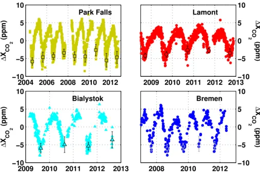
wherex is the fractional year (e.g. 2009.62). The coe_fficients calculated for each time series are in Table 3. The date of the seasonal cycle minimum for each data set is set by the local minimum in the fitted curves. Figure 1 shows the time series at Park Falls,

15

Lamont, Bia_łystok and Bremen measured by the TCCON instruments. Overlaid are the fitted curves for each time series. Figure 2 shows the time series detrended using the ESRL global annual growth rates, marking the date of the seasonal cycle minimum with symbols.

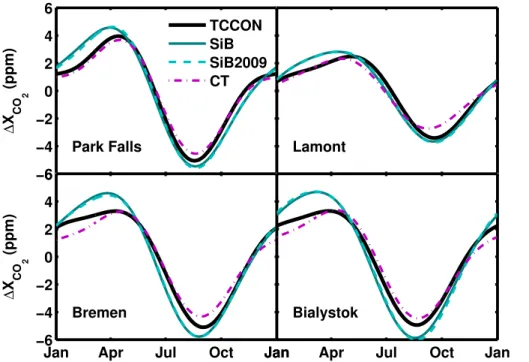
To assess how well the models compare with the TCCON data, we follow Yang et al.

20

(2007) and use a least squares fit to find the amplitude and phase that minimizes di_fferences between the seasonal cycles computed from the models and the TCCON data. Figure 3 shows the detrended seasonal cycles from the fitted curves (i.e. the

(9)

ACPD

13, 10263–10301, 2013

D. Wunch et al.

Title Page

Tables Figures

◭ ◮

Back Close

Full Screen / Esc

Discussion

P

a

per

|

Dis

cussion

P

a

per

|

Discussion

P

a

per

|

Discussio

n

P

a

per

|

the amplitudes of the SiBX_CO

2 seasonal cycles are too large by ∼10–20 %, but show good agreement in the timing of the seasonal cycle (within 7 days). The amplitudes and time lags from the CTX_CO₂ seasonal cycles match the TCCON data well, with the exception of a 9 day time lag at Lamont (Table 4).

The seasonal cycle minimum value (which we will call the “drawdown value”) is

deter-5

mined by subtracting the fitted curves from the time series, and averaging the resulting

∆X_CO

2 within ±15 days of the seasonal cycle minimum. The reported errors on the drawdown value represent the standard deviation (1σ) of the measurements. In years with fewer than 3 days of measurements near the seasonal cycle minimum, this av-eraging date range is extended to be within±25 days (Białystok and Bremen data in

10

2010). The errors for these data points are tripled to reflect the additional uncertainty. To investigate the impact of the individual CT2011 modules (fires, fossil fuels, ter-restrial biosphere, ocean) on the CTX_CO

2 interannual variability, the fitting method de-scribed above (Eq. (2)) is not used, because the ESRL growth rate is only applicable to the total CO₂, and there may be no periodicity to some of the individual components.

15

The∆CTXmodule_CO

2 anomalies are instead computed by subtracting a yearly∆CTX

module CO2 mean that has been linearly interpolated to each time step. The drawdown values are the averages of these anomalies within_±15 days of the seasonal cycle minimum in to-tal CTX_CO₂. The standard deviation of those values from year to year is then computed to estimate the interannual variability.

20

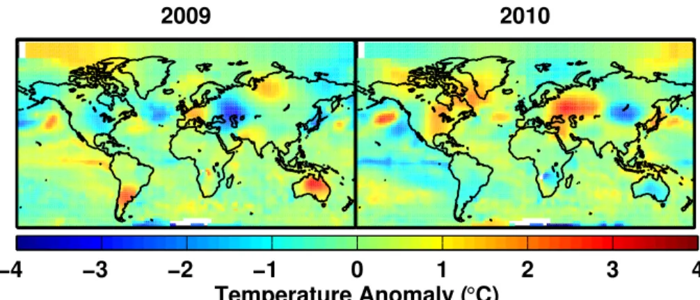
The calculated drawdown values are compared with August surface temperature measurements from the Goddard Institute for Space Science Surface Temperature Analysis (Hansen and Sato, 2004, http://data.giss.nasa.gov/gistemp/maps/). We use the 2004–2010 mean temperatures to compute surface temperature anomalies (_∆T) for years 2000–2012. The temperature anomalies are persistent: the July values and

25

patterns are similar to August. Figure 4 shows the 2009 and 2010 August temperature anomalies as examples. As we wish to evaluate the coupling between the X_CO

(10)

ACPD

13, 10263–10301, 2013

D. Wunch et al.

Title Page

Tables Figures

◭ ◮

Back Close

Full Screen / Esc

Discussion

P

a

per

|

Dis

cussion

P

a

per

|

Discussion

P

a

per

|

Discussio

n

P

a

per

|

These values are then divided by the 2009 integrated growing season (June, July, and August) ecosystem respiration between 30–60◦_{N to compute a respiration-weighted}

temperature anomaly, δT, for each year y. This weights the temperature anomalies more strongly in locations where the biosphere is active, and de-weights regions in which the biosphere is less active (i.e. over barren or snow-covered areas).

5

δT_y =

180◦_E P

j=180◦_W 60◦_N

P

i=30◦_N

R_e2009GS_{i j} ∆T_{i j}y∆a_{i j}

180P◦_E

j=180◦_W 60P◦_N

i=30◦_N

Re2009GS_{i j} ∆ai j

(3)

wherei is the latitude, j is the longitude,_∆ai j is the grid area (in m2). The value δT has units of temperature (K).

7 Results and discussion

Figure 2 shows the detrended X_CO

2, revealing clear interannual differences in the XCO2

10

seasonal cycle minima that occur in late summer to early autumn. The sites show sim-ilar patterns: 2007 and 2010 have relatively weak drawdowns, whereas 2008 and 2009 have relatively strong drawdowns. Surface temperature anomalies show that years 2007 and 2010 have relatively warm summertime mid latitudes, and 2008 and 2009 relatively cool.

15

The correlation between the drawdown value and respiration-weighted temperature anomaly for the four TCCON data sets is plotted in Fig. 5 and the slopes (∂∆_∂δTXCO2) are listed in Table 5. The slope of the relationship between the drawdown value and temper-ature anomaly for Park Falls, Białystok, Bremen and Lamont are consistent within their standard errors, giving a weighted average of 1.3_±0.7 ppm K−1_{. The Bremen slope is} 20

(11)

ACPD

13, 10263–10301, 2013

D. Wunch et al.

Title Page

Tables Figures

◭ ◮

Back Close

Full Screen / Esc

Discussion

P

a

per

|

Dis

cussion

P

a

per

|

Discussion

P

a

per

|

Discussio

n

P

a

per

|

with surface temperatures that could be caused by Bremen’s proximity to urban fos-sil fuel emissions, or its meteorological location. Excluding Bremen from the weighted mean results in an average of 1.5_±0.8 ppm K−1_{. The Bia}

łystok slope is consistent with the Park Falls and Lamont slopes, but due to low data yields during the summertimes of 2010 and 2012, the error in the estimated slope is large. The standard errors are

5

generally large at all sites because there is significant day-to-day variability in X_CO 2 near the seasonal cycle minimum due to the influence of synoptic-scale activity on the measured X_CO

2 (Keppel-Aleks et al., 2012). Figure 6 illustrates this increased sum-mertime synoptic-scale “noise”. In the sumsum-mertime, air that has originated from the north (cooler air) tends to have lower X_CO₂ values, whereas air that originated from

10

the south (warmer air) has higher X_CO

2 values, giving rise to high variability in XCO2 in the growing season. Covariations between the drawdown values and 30–60◦N sur-face temperatures (not weighted byR_e) show larger relative errors on the slopes, but consistent slope values (within error).

It is not robust to compute covariations from the ACOS-GOSAT retrievals over these

15

four locations for only two years, but the _∆X_CO

2 values from GOSAT agree with the TCCON values well within the errors for 2009 and 2010. More revealing is the spatial distribution of the GOSAT ∆X_CO

2−δT ratios between 2009 and 2010 (Fig. 7). The spatial pattern is mostly uniform, except near the oceans. This is consistent with our understanding that X_CO

2has a very large spatial footprint that is essentially hemispheric

20

on seasonal time scales. The cause of this spatial variability near the coasts is unclear. The significant correlation of X_CO

2 with temperature could point to a large-scale dynamical e_ffect, fires, fossil fuel use, or a biospheric reaction to the temperature changes. It is unlikely to be related to oceanic fluxes, as the interannual variability in CO₂from ocean fluxes is negligible (Table 6). The possible e_ffects and an estimate

25

(12)

ACPD

13, 10263–10301, 2013

D. Wunch et al.

Title Page

Tables Figures

◭ ◮

Back Close

Full Screen / Esc

Discussion

P

a

per

|

Dis

cussion

P

a

per

|

Discussion

P

a

per

|

Discussio

n

P

a

per

|

7.1 Dynamics

Variability in the dynamical mixing of CO₂ within and between the mid latitudes and the tropics is expected to be correlated with surface temperature changes, since the meridional thermal structure both responds to and drives north-south transport of air (Trenberth, 1990; Webster, 1981). Therefore, it is plausible that the slopes seen in the

5

TCCON and GOSAT data are influenced by interannual variability in the atmospheric mixing. To test this, we use the GEOS-Chem dynamical fields with static SiB 2009 bio-spheric fluxes, holding the NEE cycle constant from year to year. The results are shown in the bottom right panel of Fig. 5 and in Table 5. The SiB run with 2009 fluxes shows a weakly positive slope that is∼40 % (±40 %) of that observed, indicating that

variabil-10

ity in the mixing does contribute to the observed interannual variability in X_CO

2 minima. Because the covariations are computed with column-averaged CO₂, which is less influ-enced by local dynamics, this suggests that large-scale dynamics are important: warm years are associated with enhanced poleward transport of high CO₂ air from the sub-tropics and/or reduced equatorward transport of low CO₂ air from the Arctic, and the

15

converse for cool years.

7.2 Fires

High temperature (and lower humidity) conditions might be expected to be correlated with wild fire activity (e.g. Westerling et al., 2006) and therefore increased atmospheric CO₂ (Zhao and Running, 2010). To investigate whether variations in fires have a

sig-20

nificant e_ffect on the variations in X_CO

2 seasonal cycle minima, we analyze TCCON measurements of X_CO, a fire tracer measured simulateously with the X_CO₂. The anoma-lies in X_CO are calculated in an identical manner to X_CO

2, except that we do not use the ESRL CO₂mean growth rate, but fit an additional linear increase parameter (αx). Following Akagi et al. (2011), we assume that the modified combustion efficiency of

25

producing CO₂ from biomass burning is ∼88 % in the boreal forest, and we convert the measured_∆X_COat the time of the X_CO

(13)

ACPD

13, 10263–10301, 2013

D. Wunch et al.

Title Page

Tables Figures

◭ ◮

Back Close

Full Screen / Esc

Discussion

P

a

per

|

Dis

cussion

P

a

per

|

Discussion

P

a

per

|

Discussio

n

P

a

per

|

fires. We show the relationship between ∆X_CO

2 caused by fires with the respiration-weighted temperature anomaly in Fig. 8. The variability in _∆X_CO

2 caused by fires is at most _∼0.05 ppm K−1_{. Although CO is not a conserved tracer (its oxidation by OH}

leads to a lifetime of ∼1–2 months (Yurganov et al., 2004)), the small slope, even if a lower bound, suggests that fire does not contribute significantly to the observed

5

∼1.3 ppm K−1variability.

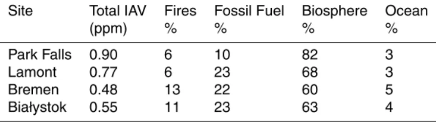
Consistently, the CT2011 fire signature (CTXfires_CO

2) accounts for only 6–13 % of the total interannual variability in summertime drawdown CTX_CO₂ in CarbonTracker (see Table 6). The fire anomalies (_∆CTXfires_CO

2) have a weak relationship with the respiration-weighted temperature anomalies (Fig. 8), and a maximum slope of∼0.05 ppm K−1.

10

7.3 Fossil fuel

The fossil fuel contribution (CTXff_CO

2) to the CTXCO2 contains significant interannual variability (_∼23 % in Lamont, Bremen and Bia_łystok, and _∼10 % in Park Falls, see Table 6). Because we detrend the TCCON data and CT2011 assimilation output of total X_CO

2 by the annual measured CO2 growth rate, much of the variability in the annual

15

fossil fuel emissions will be removed from the_∆X_CO

2 anomalies and will not contribute to the∆X_CO₂−δT slope. Any remaining variability attributed to the fossil fuel signature is likely due partially to the dynamical effects described in Sect. 7.1. The CT2011 fossil fuel signal (CTXff_CO

2) is not correlated with the respiration-weighted surface temperature (Fig. 8, bottom panel).

20

7.4 NEE

The most significant contribution to interannual variability in CTX_CO

2 is the terrestrial biosphere component, which accounts for 60 % in Bremen, increasing to 82 % in Park Falls (see Table 6). Respiration is directly influenced by surface temperature, and GPP is indirectly influenced by temperature through soil moisture. In SiB, both ecosystem

(14)

ACPD

13, 10263–10301, 2013

D. Wunch et al.

Title Page

Tables Figures

◭ ◮

Back Close

Full Screen / Esc

Discussion

P

a

per

|

Dis

cussion

P

a

per

|

Discussion

P

a

per

|

Discussio

n

P

a

per

|

respiration and GPP cause interannual variability in SiBX_CO

2. For example, the 2006 and 2009 SiBX_CO

2 seasonal cycle minima are similarly deep compared with 2010, and possess a similar growing season NEE. In 2006, the NEE was more negative relative to 2010 due to a decrease in respiration throughout the growing season. In contrast, in 2009, this was due to an increase in GPP relative to 2010. However, only

5

the interannual variability in the integrated growing season ecosystem respiration is significantly correlated with the surface temperature anomalies (R2∼0.9, Fig. 9). The interannual variability in growing season GPP is not correlated withδT, suggesting that

R_eis by far the stronger driver of this∆X_CO₂−δT relationship in SiB. This is consistent with the results of Vuki´cevi´c et al. (2003), who show that the temperature sensitivity of

10

GPP is less than that of respiration in all versions of their model. However, “greenness” indices of plant phenology (such as NDVI) have been shown to be poor predictors of GPP in the boreal coniferous region in winter and during cloudy periods (Wang et al., 2004).

NEE depends on soil moisture through GPP and/orR_e(Raich et al., 1991; Denning

15

et al., 1996; Zhao and Running, 2010). To evaluate this, we use the global gridded Palmer Drought Severity Index (PDSI, Dai et al., 2004; Dai, 2011a,b), which is avail-able through 2010. PDSI values that are negative indicate dry conditions, and positive indices indicate wet conditions. Annual averages of PDSI from 30◦N–60◦N weakly cor-relate withδT (R2=0.33) for the years 2004–2010. However, it is di_fficult to determine

20

whether the X_CO

2 drawdown values from the TCCON measurements correlate signifi-cantly with PDSI. Only the Park Falls dataset has sufficient overlap with the available PDSI values, and it has a negative slope (drier conditions yield higher X_CO

2 values). The other sites, even if they possess more than two years of coincident measurements, do not encompass a sufficiently large PDSI range to compute significant slopes.

(15)

ACPD

13, 10263–10301, 2013

D. Wunch et al.

Title Page

Tables Figures

◭ ◮

Back Close

Full Screen / Esc

Discussion

P

a

per

|

Dis

cussion

P

a

per

|

Discussion

P

a

per

|

Discussio

n

P

a

per

|

8 Summary and future study

Interannual variability in the seasonal cycle minima of column-averaged dry-air mole fractions of CO₂is correlated with summertime surface temperature anomalies at bo-real latitudes. The CarbonTracker 2011 assimilation and GEOS-Chem simulations sug-gest that this relationship is caused both by dynamical mixing and biospheric activity,

5

in roughly equal proportion. The effects of emissions from fossil fuel combustion and fires appear to be small and uncorrelated with surface temperature. However, CT2011 and the GEOS-Chem driven SiB∆X_CO₂−δT relationships are generally weaker than observed.

It is clear that there are several avenues worth pursuing to further investigate the

10

∆X_CO₂−δT relationship. It is important to try other realizations of the dynamics: using different transport models such as TM5, or different underlying wind fields, such as ECMWF or NCEP. Because our results are derived from column-averaged atmospheric CO₂measurements, which are relatively insensitive to planetary boundary layer (local) dynamics, we anticipate that differences in the large-scale dynamics will dominate the

15

variability.

To further disentangle the e_ffects of NEE on the observed variability, both the e_ffects of GPP andR_e should be probed. Although interannual variability in GPP is not cor-related withδT in SiB, Guerlet et al. (2013) have attributed the interannual variability in the GOSAT 2009–2010 seasonal cycles to reduced carbon uptake (GPP) through

20

their inversions. However, the 2010 Northern Hemisphere had exceptional warming, causing record-breaking heatwaves throughout eastern Europe and Russia, and fires in western Russia (Barriopedro et al., 2011). The correlation between δT and GPP should be explored in other biospheric models, and by using chlorophyll fluorescence (e.g. Frankenberg et al., 2011) instead of, or in conjunction with, the current proxies

25

(16)

ACPD

13, 10263–10301, 2013

D. Wunch et al.

Title Page

Tables Figures

◭ ◮

Back Close

Full Screen / Esc

Discussion

P

a

per

|

Dis

cussion

P

a

per

|

Discussion

P

a

per

|

Discussio

n

P

a

per

|

Developing robust metrics for respiration and GPP responses to temperature is crit-ical for reducing uncertainties in Earth system models and for diagnosing the vulnera-bility of permafrost carbon pools to future change.

Acknowledgements. CarbonTracker 2011 results were provided by NOAA ESRL, Boulder, Col-orado, USA from the website at http://carbontracker.noaa.gov. US funding for TCCON comes

5

from NASA’s Carbon Cycle Program, grant number NNX11AG01G, the Orbiting Carbon Ob-servatory Program, and the DOE/ARM Program. We acknowledge financial support of the Białystok TCCON site from the Senate of Bremen and EU projects IMECC and GEOmon as well as maintenance and logistical work provided by AeroMeteo Service. POW and JTR receive support from NASA’s Carbon Cycle Science program (NNX10AT83G). The GOSAT XCO2 data

10

were obtained from the Atmospheric CO₂Observations from Space (ACOS) project. We thank the Japanese three parties (NIES, JAXA, MOE) for making the GOSAT spectra available to the scientific community. Self-calibrated PDSI data with Penman-Monteith PE were downloaded from http://www.cgd.ucar.edu/cas/catalog/climind/pdsi.html.

References

15

Akagi, S. K., Yokelson, R. J., Wiedinmyer, C., Alvarado, M. J., Reid, J. S., Karl, T., Crounse, J. D., and Wennberg, P. O.: Emission factors for open and domestic biomass burning for use in atmospheric models, Atmos. Chem. Phys., 11, 4039–4072, doi:10.5194/acp-11-4039-2011, 2011. 10274

Baker, I. T., Prihodko, L., Denning, A. S., Goulden, M., Miller, S., and da Rocha, H. R.: Seasonal

20

drought stress in the Amazon: reconciling models and observations, J. Geophys. Res., 113, G00B01, doi:10.1029/2007JG000644, 2008. 10269

Baker, I. T., Denning, A. S., and St ¨ockli, R.: North American gross primary productivity: re-gional characterization and interannual variability, Tellus B, 62, 533–549, doi:10.1111/j.1600-0889.2010.00492.x, 2010. 10269

25

Barriopedro, D., Fischer, E. M., Luterbacher, J., Trigo, R. M., and Garc´ıa-Herrera, R.: The hot summer of 2010: redrawing the temperature record map of Europe, Science, 332, 220–224, doi:10.1126/science.1201224, 2011. 10277

Boden, T. A., Marland, G., and Andres, R. J.: Global, Regional, and National Fossil-Fuel CO2

Emissions, doi:10.3334/CDIAC/00001 V2011, Carbon Dioxide Information Analysis Center,

(17)

ACPD

13, 10263–10301, 2013

D. Wunch et al.

Title Page

Tables Figures

◭ ◮

Back Close

Full Screen / Esc

Discussion

P

a

per

|

Dis

cussion

P

a

per

|

Discussion

P

a

per

|

Discussio

n

P

a

per

|

Oak Ridge National Laboratory, US Department of Energy, Oak Ridge, Tenn., USA, 2011. 10268

Braswell, B. H., Schimel, D. S., Linder, E., and Moore, B.: The response of global terrestrial ecosystems to interannual temperature variability, Science, 278, 870–873, doi:10.1126/science.278.5339.870, 1997. 10264

5

CarbonTracker: Documentation – CT2011, Tech. rep., Earth System Research Laboratory – National Oceanic and Atmospheric Administration, available at: http://www.esrl.noaa.gov/ gmd/ccgg/carbontracker/documentation obs.html, 2011. 10266, 10267, 10268

Conway, T. and Tans, P.: Annual mean global carbon dioxide growth rates, available at: http:// www.esrl.noaa.gov/gmd/ccgg/trends/global.html, NOAA/ESRL, last access: 7 January 2013.

10

10270

Crisp, D., Fisher, B. M., O’Dell, C., Frankenberg, C., Basilio, R., B ¨osch, H., Brown, L. R., Cas-tano, R., Connor, B., Deutscher, N. M., Eldering, A., Griffith, D., Gunson, M., Kuze, A., Man-drake, L., McDuffie, J., Messerschmidt, J., Miller, C. E., Morino, I., Natraj, V., Notholt, J., O’Brien, D. M., Oyafuso, F., Polonsky, I., Robinson, J., Salawitch, R., Sherlock, V., Smyth, M.,

15

Suto, H., Taylor, T. E., Thompson, D. R., Wennberg, P. O., Wunch, D., and Yung, Y. L.: The ACOS CO2 retrieval algorithm – Part II: Global XCO2 data characterization, Atmos. Meas.

Tech., 5, 687–707, doi:10.5194/amt-5-687-2012, 2012. 10267

Dai, A.: Characteristics and trends in various forms of the Palmer Drought Severity Index during 1900–2008, J. Geophys. Res., 116, D12115, doi:10.1029/2010JD015541, 2011a. 10276

20

Dai, A.: Drought under global warming: a review, Wiley Interdisciplinary Reviews, Climate Change, 2, 45–65, doi:10.1002/wcc.81, 2011b. 10276

Dai, A., Trenberth, K. E., and Qian, T.: A global dataset of Palmer Drought Severity Index for 1870–2002: relationship with soil moisture and effects of surface warming, J. Hydrometeorol., 5, 1117–1130, doi:10.1175/JHM-386.1, 2004. 10276

25

D’Arrigo, R., Jacoby, G. C., and Fung, I. Y.: Boreal forests and atmosphere-biosphere exchange of carbon dioxide, Nature, 329, 321–323, doi:10.1038/329321a0, 1987. 10265

Denning, A. S., Collatz, G. J., Zhang, C., Randall, D. A., Berry, J. A., Sellers, P. J., Colello, G. D., and Dazlich, D. A.: Simulations of terrestrial carbon metabolism and atmospheric CO2

in a general circulation model, Part 1: Surface carbon fluxes, Tellus B, 48, 521–542,

30

doi:10.1034/j.1600-0889.1996.t01-2-00009.x, 1996. 10269, 10276

(18)

ACPD

13, 10263–10301, 2013

D. Wunch et al.

Title Page

Tables Figures

◭ ◮

Back Close

Full Screen / Esc

Discussion

P

a

per

|

Dis

cussion

P

a

per

|

Discussion

P

a

per

|

Discussio

n

P

a

per

|

Frankenberg, C., Fisher, J. B., Worden, J., Badgley, G., Saatchi, S. S., Lee, J.-E., Toon, G. C., Butz, A., Jung, M., Kuze, A., and Yokota, T.: New global observations of the terrestrial carbon cycle from GOSAT: patterns of plant fluorescence with gross primary productivity, Geophys. Res. Lett., 38, 1–6, doi:10.1029/2011GL048738, 2011. 10277

Fung, I. Y., Tucker, C. J., and Prentice, K. C.: Application of advanced very high resolution

5

radiometer vegetation index to study atmosphere–biosphere exchange of CO2, J. Geophys.

Res., 92, 2999–3015, doi:10.1029/JD092iD03p02999, 1987. 10265

Giglio, L., van der Werf, G. R., Randerson, J. T., Collatz, G. J., and Kasibhatla, P.: Global estimation of burned area using MODIS active fire observations, Atmos. Chem. Phys., 6, 957–974, doi:10.5194/acp-6-957-2006, 2006. 10268

10

Guerlet, S., Basu, S., Butz, A., Krol, M., Hahne, P., Houweling, S., Hasekamp, O. P., and Aben, I.: Reduced carbon uptake during the 2010 Northern Hemisphere summer as ob-served from GOSAT, Geophys. Res. Lett., in press, doi:10.1002/grl.50402, 2013. 10265, 10277

Hamazaki, T.: Fourier transform spectrometer for Greenhouse Gases Observing Satellite

15

(GOSAT), P. SPIE Is. & T. Elect., 5659, 73–80, doi:10.1117/12.581198, 2005. 10265 Hansen, J. and Sato, M.: Greenhouse gas growth rates., P. Natl. Acad. Sci. USA, 101, 16109–

16114, doi:10.1073/pnas.0406982101, 2004. 10271

Houghton, R. A.: Interannual variability in the global carbon cycle, J. Geophys. Res., 105, 20121–20130, doi:10.1029/2000JD900041, 2000. 10264

20

Jacobson, A. R., MikaloffFletcher, S. E., Gruber, N., Sarmiento, J. L., and Gloor, M.: A joint atmosphere-ocean inversion for surface fluxes of carbon dioxide: 1. Methods and global-scale fluxes, Global Biogeochem. Cy., 21, GB1019, doi:10.1029/2005GB002556, 2007. 10268

Keppel-Aleks, G., Wennberg, P. O., and Schneider, T.: Sources of variations in total column

25

carbon dioxide, Atmos. Chem. Phys., 11, 3581–3593, doi:10.5194/acp-11-3581-2011, 2011. 10265

Keppel-Aleks, G., Wennberg, P. O., Washenfelder, R. A., Wunch, D., Schneider, T., Toon, G. C., Andres, R. J., Blavier, J.-F., Connor, B., Davis, K. J., Desai, A. R., Messerschmidt, J., Notholt, J., Roehl, C. M., Sherlock, V., Stephens, B. B., Vay, S. A., and Wofsy, S. C.: The

30

(19)

ACPD

13, 10263–10301, 2013

D. Wunch et al.

Title Page

Tables Figures

◭ ◮

Back Close

Full Screen / Esc

Discussion

P

a

per

|

Dis

cussion

P

a

per

|

Discussion

P

a

per

|

Discussio

n

P

a

per

|

Keppel-Aleks, G., Randerson, J. T., Lindsay, K., Stephens, B. B., Moore, J. K., Doney, S. C., Thornton, P. E., Mahowald, N. M., Hoffman, F. M., Sweeney, C., Tans, P. P., Wennberg, P. O., and Wofsy, S. C.: Atmospheric carbon dioxide variability in the Community Earth System Model: evaluation and transient dynamics during the 20th and 21st centuries, J. Climate, in press, 2013. 10266

5

Krol, M., Houweling, S., Bregman, B., van den Broek, M., Segers, A., van Velthoven, P., Peters, W., Dentener, F., and Bergamaschi, P.: The two-way nested global chemistry-transport zoom model TM5: algorithm and applications, Atmos. Chem. Phys., 5, 417–432, doi:10.5194/acp-5-417-2005, 2005. 10267

Lloyd, J. and Taylor, J. A.: On the temperature dependence of soil respiration, Funct. Ecol., 8,

10

315, doi:10.2307/2389824, 1994. 10265

Machta, L.: Mauna Loa and global trends in air quality, B. Am. Meteorol. Soc., 53, 402–420, doi:10.1175/1520-0477(1972)053<0402:MLAGTI>2.0.CO;2, 1972. 10265

Messerschmidt, J., Geibel, M. C., Blumenstock, T., Chen, H., Deutscher, N. M., Engel, A., Feist, D. G., Gerbig, C., Gisi, M., Hase, F., Katrynski, K., Kolle, O., Lavriˇc, J. V., Notholt, J.,

15

Palm, M., Ramonet, M., Rettinger, M., Schmidt, M., Sussmann, R., Toon, G. C., Truong, F., Warneke, T., Wennberg, P. O., Wunch, D., and Xueref-Remy, I.: Calibration of TCCON column-averaged CO2: the first aircraft campaign over European TCCON sites, Atmos.

Chem. Phys., 11, 10765–10777, doi:10.5194/acp-11-10765-2011, 2011. 10266

Messerschmidt, J., Chen, H., Deutscher, N. M., Gerbig, C., Grupe, P., Katrynski, K., Koch, F.-T.,

20

Lavriˇc, J. V., Notholt, J., R ¨odenbeck, C., Ruhe, W., Warneke, T., and Weinzierl, C.: Automated ground-based remote sensing measurements of greenhouse gases at the Białystok site in comparison with collocated in situ measurements and model data, Atmos. Chem. Phys., 12, 6741–6755, doi:10.5194/acp-12-6741-2012, 2012a. 10266

Messerschmidt, J., Parazoo, N., Deutscher, N. M., Roehl, C., Warneke, T., Wennberg, P. O., and

25

Wunch, D.: Evaluation of atmosphere-biosphere exchange estimations with TCCON mea-surements, Atmos. Chem. Phys. Discuss., 12, 12759–12800, doi:10.5194/acpd-12-12759-2012, 2012b. 10269

Molteni, F., Buizza, R., Palmer, T. N., and Petroliagis, T.: The ECMWF ensemble pre-diction system: methodology and validation, Q. J. Roy. Meteor. Soc., 122, 73–119,

30

doi:10.1002/qj.49712252905, 1996. 10268

(20)

ACPD

13, 10263–10301, 2013

D. Wunch et al.

Title Page

Tables Figures

◭ ◮

Back Close

Full Screen / Esc

Discussion

P

a

per

|

Dis

cussion

P

a

per

|

Discussion

P

a

per

|

Discussio

n

P

a

per

|

and Wennberg, P. O.: Daily and 3-hourly variability in global fire emissions and consequences for atmospheric model predictions of carbon monoxide, J. Geophys. Res., 116, D24303, doi:10.1029/2011JD016245, 2011. 10268

Nassar, R., Jones, D. B. A., Suntharalingam, P., Chen, J. M., Andres, R. J., Wecht, K. J., Yantosca, R. M., Kulawik, S. S., Bowman, K. W., Worden, J. R., Machida, T., and

Mat-5

sueda, H.: Modeling global atmospheric CO2 with improved emission inventories and CO2

production from the oxidation of other carbon species, Geosci. Model Dev., 3, 689–716, doi:10.5194/gmd-3-689-2010, 2010. 10269

O’Dell, C. W., Connor, B., B ¨osch, H., O’Brien, D., Frankenberg, C., Castano, R., Christi, M., Eldering, D., Fisher, B., Gunson, M., McDuffie, J., Miller, C. E., Natraj, V., Oyafuso, F.,

Polon-10

sky, I., Smyth, M., Taylor, T., Toon, G. C., Wennberg, P. O., and Wunch, D.: The ACOS CO2

retrieval algorithm – Part 1: Description and validation against synthetic observations, Atmos. Meas. Tech., 5, 99–121, doi:10.5194/amt-5-99-2012, 2012. 10267

Parazoo, N. C., Denning, A. S., Kawa, S. R., Corbin, K. D., Lokupitiya, R. S., and Baker, I. T.: Mechanisms for synoptic variations of atmospheric CO2 in North America, South

Amer-15

ica and Europe, Atmos. Chem. Phys., 8, 7239–7254, doi:10.5194/acp-8-7239-2008, 2008. 10269

Peters, W., Jacobson, A. R., Sweeney, C., Andrews, A. E., Conway, T. J., Masarie, K., Miller, J. B., Bruhwiler, L. M. P., P ´etron, G., Hirsch, A. I., Worthy, D. E. J., van der Werf, G. R., Randerson, J. T., Wennberg, P. O., Krol, M. C., and Tans, P. P.: An atmospheric perspective

20

on North American carbon dioxide exchange: CarbonTracker, P. Natl. Acad. Sci. USA, 104, 18925–18930, doi:10.1073/pnas.0708986104, 2007. 10267

Piao, S., Ciais, P., Friedlingstein, P., Peylin, P., Reichstein, M., Luyssaert, S., Margolis, H., Fang, J., Barr, A., Chen, A., Grelle, A., Hollinger, D. Y., Laurila, T., Lindroth, A., Richard-son, A. D., and Vesala, T.: Net carbon dioxide losses of northern ecosystems in response to

25

autumn warming, Nature, 451, 49–52, doi:10.1038/nature06444, 2008. 10265

Potter, C. S., Randerson, J. T., Field, C. B., Matson, P. A., Vitousek, P. M., Mooney, H. A., and Klooster, S. A.: Terrestrial ecosystem production: a process model based on global satellite and surface data, Global Biogeochem. Cy., 7, 811, doi:10.1029/93GB02725, 1993. 10268 Raich, J. W. and Schlesinger, W. H.: The global carbon dioxide flux in soil respiration and its

30

(21)

ACPD

13, 10263–10301, 2013

D. Wunch et al.

Title Page

Tables Figures

◭ ◮

Back Close

Full Screen / Esc

Discussion

P

a

per

|

Dis

cussion

P

a

per

|

Discussion

P

a

per

|

Discussio

n

P

a

per

|

Raich, J. W., Rastetter, E. B., Melillo, J. M., Kicklighter, D. W., Steudler, P. A., Peterson, B. J., Grace, A. L., III, B. M., and Vorosmarty, C. J.: Potential net primary productivity in South America: application of a global model, Ecol. Appl., 1, 399, doi:10.2307/1941899, 1991. 10269, 10276

Randerson, J. T., Thompson, M. V., Conway, T. J., Fung, I. Y., and Field, C. B.: The contribution

5

of terrestrial sources and sinks to trends in the seasonal cycle of atmospheric carbon dioxide, Global Biogeochem. Cy., 11, 535–560, doi:10.1029/97GB02268, 1997. 10264, 10265, 10268 Randerson, J. T., Field, C. B., Fung, I. Y., and Tans, P. P.: Increases in early season ecosystem uptake explain recent changes in the seasonal cycle of atmospheric CO₂at high northern latitudes, Geophys. Res. Lett., 26, 2765, doi:10.1029/1999GL900500, 1999. 10265

10

Rodgers, C. D. and Connor, B. J.: Intercomparison of remote sounding instruments, J. Geophys. Res., 108, 4116, doi:10.1029/2002JD002299, 2003. 10269

Sellers, P., Randall, D., Collatz, G., Berry, J., Field, C., Dazlich, D., Zhang, C., Col-lelo, G., and Bounoua, L.: A revised land surface parameterization (SiB2) for atmo-spheric GCMS, Part I: Model formulation, J. Climate, 9, 676–705,

doi:10.1175/1520-15

0442(1996)009<0676:ARLSPF>2.0.CO;2, 1996a. 10266, 10269

Sellers, P. J., Tucker, C. J., Collatz, G. J., Los, S. O., Justice, C. O., Dazlich, D. A., and Ran-dall, D. A.: A revised land surface parameterization (SiB2) for atmospheric GCMS, Part II: The generation of global fields of terrestrial biophysical parameters from satellite data, J. Climate, 9, 706–737, doi:10.1175/1520-0442(1996)009<0706:ARLSPF>2.0.CO;2, 1996b. 10269

20

Suntharalingam, P., Spivakovsky, C. M., Logan, J. A., and McElroy, M. B.: Estimating the distribution of terrestrial CO2 sources and sinks from atmospheric measurements:

sensitivity to configuration of the observation network, J. Geophys. Res., 108, 4452, doi:10.1029/2002JD002207, 2003. 10269

Suntharalingam, P., Jacob, D. J., Palmer, P. I., Logan, J. A., Yantosca, R. M., Xiao, Y.,

25

Evans, M. J., Streets, D. G., Vay, S. L., and Sachse, G. W.: Improved quantification of Chinese carbon fluxes using CO2/CO correlations in Asian outflow, J. Geophys. Res., 109, D18S18,

doi:10.1029/2003JD004362, 2004. 10269

Takahashi, T., Sutherland, S. C., Wanninkhof, R., Sweeney, C., Feely, R. a., Chipman, D. W., Hales, B., Friederich, G., Chavez, F., Sabine, C., Watson, A., Bakker, D. C., Schuster, U.,

30

(22)

ACPD

13, 10263–10301, 2013

D. Wunch et al.

Title Page

Tables Figures

◭ ◮

Back Close

Full Screen / Esc

Discussion

P

a

per

|

Dis

cussion

P

a

per

|

Discussion

P

a

per

|

Discussio

n

P

a

per

|

decadal change in surface oceanpCO2, and net sea-air CO2 flux over the global oceans,

Deep Sea Res. Pt. II, 56, 554–577, doi:10.1016/j.dsr2.2008.12.009, 2009. 10268

Trenberth, K. E.: Recent observed interdecadal climate changes in the North-ern Hemisphere, B. Am. Meteor. Soc., 71, 988–993, doi:10.1175/1520-0477(1990)071<0988:ROICCI>2.0.CO;2, 1990. 10274

5

Uppala, S. M., K ˚allberg, P. W., Simmons, A. J., Andrae, U., Bechtold, V. D. C., Fiorino, M., Gib-son, J. K., Haseler, J., Hernandez, A., Kelly, G. A., Li, X., Onogi, K., Saarinen, S., Sokka, N., Allan, R. P., Andersson, E., Arpe, K., Balmaseda, M. A., Beljaars, A. C. M., Berg, L. V. D., Bidlot, J., Bormann, N., Caires, S., Chevallier, F., Dethof, A., Dragosavac, M., Fisher, M., Fuentes, M., Hagemann, S., H ´olm, E., Hoskins, B. J., Isaksen, L., Janssen, P. A. E. M.,

10

Jenne, R., Mcnally, A. P., Mahfouf, J.-F., Morcrette, J.-J., Rayner, N. A., Saunders, R. W., Simon, P., Sterl, A., Trenberth, K. E., Untch, A., Vasiljevic, D., Viterbo, P., and Woollen, J.: The ERA-40 re-analysis, Q. J. Roy. Meteor. Soc., 131, 2961–3012, doi:10.1256/qj.04.176, 2005. 10268

van der Werf, G. R., Randerson, J. T., Giglio, L., Collatz, G. J., Mu, M., Kasibhatla, P. S.,

Mor-15

ton, D. C., DeFries, R. S., Jin, Y., and van Leeuwen, T. T.: Global fire emissions and the contribution of deforestation, savanna, forest, agricultural, and peat fires (1997–2009), At-mos. Chem. Phys., 10, 11707–11735, doi:10.5194/acp-10-11707-2010, 2010. 10268 Vuki´cevi´c, T., Braswell, B., and Schimel, D.: A diagnostic study of temperature controls on global

terrestrial carbon exchange, Tellus B, 53, 150–170, doi:10.1034/j.1600-0889.2001.d01-13.x,

20

2003. 10276

Wang, Q., Tenhunen, J., Dinh, N. Q., Reichstein, M., Vesala, T., and Keronen, P.: Simi-larities in ground- and satellite-based NDVI time series and their relationship to physio-logical activity of a Scots pine forest in Finland, Remote Sens. Environ., 93, 225–237, doi:10.1016/j.rse.2004.07.006, 2004. 10276

25

Washenfelder, R. A., Toon, G. C., Blavier, J.-F. L., Yang, Z., Allen, N. T., Wennberg, P. O., Vay, S. a., Matross, D. M., and Daube, B. C.: Carbon dioxide column abundances at the Wisconsin Tall Tower site, J. Geophys. Res., 111, 1–11, doi:10.1029/2006JD007154, 2006. 10266

Webster, P. J.: Mechanisms determining the atmospheric response to sea

sur-30

(23)

ACPD

13, 10263–10301, 2013

D. Wunch et al.

Title Page

Tables Figures

◭ ◮

Back Close

Full Screen / Esc

Discussion

P

a

per

|

Dis

cussion

P

a

per

|

Discussion

P

a

per

|

Discussio

n

P

a

per

|

Westerling, A. L., Hidalgo, H. G., Cayan, D. R., and Swetnam, T. W.: Warming and earlier spring increase western US forest wildfire activity, Science, 313, 940–943, doi:10.1126/science.1128834, 2006. 10274

Wunch, D., Toon, G. C., Wennberg, P. O., Wofsy, S. C., Stephens, B. B., Fischer, M. L., Uchino, O., Abshire, J. B., Bernath, P., Biraud, S. C., Blavier, J.-F. L., Boone, C.,

Bow-5

man, K. P., Browell, E. V., Campos, T., Connor, B. J., Daube, B. C., Deutscher, N. M., Diao, M., Elkins, J. W., Gerbig, C., Gottlieb, E., Griffith, D. W. T., Hurst, D. F., Jim ´enez, R., Keppel-Aleks, G., Kort, E. A., Macatangay, R., Machida, T., Matsueda, H., Moore, F., Morino, I., Park, S., Robinson, J., Roehl, C. M., Sawa, Y., Sherlock, V., Sweeney, C., Tanaka, T., and Zondlo, M. A.: Calibration of the Total Carbon Column Observing Network using aircraft

pro-10

file data, Atmos. Meas. Tech., 3, 1351–1362, doi:10.5194/amt-3-1351-2010, 2010. 10266 Wunch, D., Toon, G. C., Blavier, J.-F. L., Washenfelder, R. A., Notholt, J., Connor, B. J.,

Grif-fith, D. W. T., Sherlock, V., and Wennberg, P. O.: The total carbon column observing network, Philos. T. R. Soc. A, 369, 2087–2112, doi:10.1098/rsta.2010.0240, 2011a. 10265, 10266 Wunch, D., Wennberg, P. O., Toon, G. C., Connor, B. J., Fisher, B., Osterman, G. B.,

Franken-15

berg, C., Mandrake, L., O’Dell, C., Ahonen, P., Biraud, S. C., Castano, R., Cressie, N., Crisp, D., Deutscher, N. M., Eldering, A., Fisher, M. L., Griffith, D. W. T., Gunson, M., Heikki-nen, P., Keppel-Aleks, G., Kyr ¨o, E., Lindenmaier, R., Macatangay, R., Mendonca, J., Messer-schmidt, J., Miller, C. E., Morino, I., Notholt, J., Oyafuso, F. A., Rettinger, M., Robinson, J., Roehl, C. M., Salawitch, R. J., Sherlock, V., Strong, K., Sussmann, R., Tanaka, T.,

Thomp-20

son, D. R., Uchino, O., Warneke, T., and Wofsy, S. C.: A method for evaluating bias in global measurements of CO2 total columns from space, Atmos. Chem. Phys., 11, 12317–12337,

doi:10.5194/acp-11-12317-2011, 2011b. 10267, 10287

Yang, Z., Washenfelder, R. A., Keppel-Aleks, G., Krakauer, N. Y., Randerson, J. T., Tans, P. P., Sweeney, C., and Wennberg, P. O.: New constraints on Northern Hemisphere growing

sea-25

son net flux, Geophys. Res. Lett., 34, L12807, doi:10.1029/2007GL029742, 2007. 10270 Yokota, T., Yoshida, Y., Eguchi, N., Ota, Y., Tanaka, T., Watanabe, H., and Maksyutov, S.: Global

concentrations of CO2and CH4retrieved from GOSAT: first preliminary results, Sola, 5, 160–

163, doi:10.2151/sola.2009-041, 2009. 10265, 10267

Yurganov, L. N., Blumenstock, T., Grechko, E. I., Hase, F., Hyer, E. J., Kasischke, E. S.,

30

(24)

ACPD

13, 10263–10301, 2013

D. Wunch et al.

Title Page

Tables Figures

◭ ◮

Back Close

Full Screen / Esc

Discussion

P

a

per

|

Dis

cussion

P

a

per

|

Discussion

P

a

per

|

Discussio

n

P

a

per

|

monoxide emission anomaly in the Northern Hemisphere based on total column and surface concentration measurements, J. Geophys. Res., 109, D15305, doi:10.1029/2004JD004559, 2004. 10275

Zhao, M. and Running, S. W.: Drought-induced reduction in global terrestrial net primary pro-duction from 2000 through 2009, Science, 329, 940–943, doi:10.1126/science.1192666,

5

2010. 10274, 10276

(25)

ACPD

13, 10263–10301, 2013

D. Wunch et al.

Title Page

Tables Figures

◭ ◮

Back Close

Full Screen / Esc

Discussion

P

a

per

|

Dis

cussion

P

a

per

|

Discussion

P

a

per

|

Discussio

n

P

a

per

|

Table 1.The parameters used to minimize variability in the Southern Hemisphere, in order to re-duce the impact of the ACOS-GOSAT retrieval on the XCO2values. The model used in this case includes a small seasonal cycle in the Southern Hemisphere (i.e. Assumption 1 from Wunch et al., 2011b). The blended albedo parameter is defined as (2.4(A-band albedo)−1.13(strong CO₂-band albedo)). The ∆P parameter is defined as (P_surface−Pprior), wherePsurface is the

re-trieved surface pressure, andPprioris the a priori value from ECMWF.

parameter slope units

blended albedo 6.4±0.2 ppm (unit albedo)−1

∆P ₋0.136±0.006 ppm hPa−1

A-band albedo −10.0±0.5 ppm (unit albedo)−1 aerosol optical depth −12.7±1.2 ppm (unit aod)−1

(26)

ACPD

13, 10263–10301, 2013

D. Wunch et al.

Title Page

Tables Figures

◭ ◮

Back Close

Full Screen / Esc

Discussion

P

a

per

|

Dis

cussion

P

a

per

|

Discussion

P

a

per

|

Discussio

n

P

a

per

|

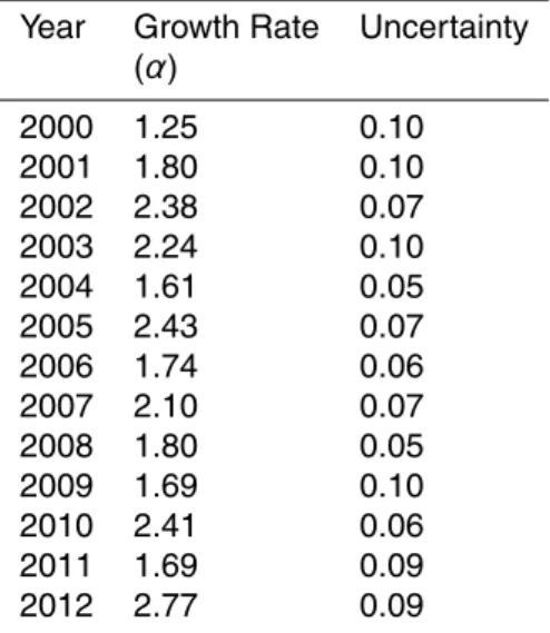
Table 2.Mean annual CO2growth rates published on the ESRL-NOAA webpage: http://www.

esrl.noaa.gov/gmd/ccgg/trends/global.html. The rates and their uncertainties are expressed in ppm yr−1

.

Year Growth Rate Uncertainty (α)

2000 1.25 0.10

2001 1.80 0.10

2002 2.38 0.07

2003 2.24 0.10

2004 1.61 0.05

2005 2.43 0.07

2006 1.74 0.06

2007 2.10 0.07

2008 1.80 0.05

2009 1.69 0.10

2010 2.41 0.06

2011 1.69 0.09

(27)

ACPD

13, 10263–10301, 2013

D. Wunch et al.

Title Page

Tables Figures

◭ ◮

Back Close

Full Screen / Esc

Discussion

P

a

per

|

Dis

cussion

P

a

per

|

Discussion

P

a

per

|

Discussio

n

P

a

per

|

Table 3.Curve fitting parameters for Eq. (2). The parametersα,a₀represent the linear secular increase:αis in ppm yr−1

anda₀is the y-intercept in ppm. Parametera₁(ppm) represents the amplitude of the cos(2πx) term, andb₁(ppm) represents the amplitude of the sin(2πx) term. Thea₂andb₂parameters are the amplitudes of the cos(4πx) and sin(4πx) terms, respectively. The drawdown date (DD) and seasonal cycle maximum date (MD) are the dates of the local minima and maxima of the fitted curves, respectively, in day of the year.

Site α a0 a1 a2 b1 b2 DD MD

Park Falls (TCCON) ESRL (see Table 2) 0.81 1.73 −0.51 3.32 −1.48 230 104 Lamont (TCCON) ESRL (see Table 2) 1.52 0.11 0.54 2.71 −0.55 262 124 Białystok (TCCON) ESRL (see Table 2) 0.59 2.32 −0.11 3.21 −1.02 232 87 Bremen (TCCON) ESRL (see Table 2) 1.37 1.64 0.39 3.62 −0.93 245 98

Park Falls (GOSAT) ESRL (see Table 2) 0.08 1.51 −1.08 3.63 −1.58 225 103 Lamont (GOSAT) ESRL (see Table 2) −0.05 0.67 0.12 2.79 −0.99 245 114 Białystok (GOSAT) ESRL (see Table 2) −0.08 2.49 0.08 2.93 −1.81 232 108 Bremen (GOSAT) ESRL (see Table 2) −0.34 1.34 −0.01 2.89 −1.57 236 114

Park Falls (SiB) 2.22 −4075.59 2.25 −0.51 4.06 −1.00 231 90 Lamont (SiB) 2.29 −4217.89 0.47 0.35 3.15 −0.39 260 102 Białystok (SiB) 2.44 −4511.29 3.26 −0.25 4.05 −0.69 229 67 Bremen (SiB) 2.27 −4169.57 2.36 −0.15 4.42 −0.90 237 85

Park Falls (SiB 2009) 2.25 −4129.40 2.14 −0.51 4.11 −1.16 232 94 Lamont (SiB 2009) 2.31 −4260.74 0.40 0.40 3.19 −0.39 261 104 Białystok (SiB 2009) 2.40 −4438.20 3.27 −0.10 4.21 −0.72 232 65 Bremen (SiB 2009) 2.29 −4216.98 2.34 −0.07 4.35 −0.97 238 87

(28)

ACPD

13, 10263–10301, 2013

D. Wunch et al.

Title Page

Tables Figures

◭ ◮

Back Close

Full Screen / Esc

Discussion

P

a

per

|

Dis

cussion

P

a

per

|

Discussion

P

a

per

|

Discussio

n

P

a

per

|

Table 4.Time lag and amplitude adjustments necessary to best fit the TCCON data with the model fits. The time lag is in days, where a positive time lag means that the model should be delayed to best fit the TCCON data. The amplitude is multiplicative, so a value less than 1 means that the model amplitude should be reduced to best fit the TCCON data. See Fig. 3 for the related figure.

Site SiB CarbonTracker

Time Lag Amplitude Time Lag Amplitude