Research Article
Bridging the Gap between Economic
Modelling and Simulation: A Simple Dynamic Aggregate
Demand-Aggregate Supply Model with Matlab
José M. Gaspar
1,21Cat´olica Porto Business School, Universidade Cat´olica Portuguesa, Porto, Portugal 2CEF.UP, University of Porto, Porto, Portugal
Correspondence should be addressed to Jos´e M. Gaspar; [email protected] Received 13 July 2017; Accepted 28 November 2017; Published 16 January 2018 Academic Editor: Oluwole D. Makinde
Copyright © 2018 Jos´e M. Gaspar. This is an open access article distributed under the Creative Commons Attribution License, which permits unrestricted use, distribution, and reproduction in any medium, provided the original work is properly cited. This paper aims to connect the bridge between analytical results and the use of the computer for numerical simulations in economics. We address the analytical properties of a simple dynamic aggregate demand and aggregate supply (AD-AS) model and solve it numerically. The model undergoes a bifurcation as its steady state smoothly interchanges stability depending on the relationship between the impact of real interest rate on demand for liquidity and how fast agents revise their expectations on inflation. Using code embedded into a unique function in Matlab, we plot the numerical solutions of the model and simulate different dynamic adjustments using different parameter values. The same function also accommodates the analysis of the impacts of fiscal and monetary policy and supply side shocks on the steady state and the transition dynamics of the model.
1. Introduction
This study seeks to provide a contribution of potential interest to researchers both within the economics profession and from different fields by highlighting the connection between analytical results and computer simulation. Our purposes are twofold: (i) we seek to show, starting from a simple dynamic inflation model used in Economics, how we can use the computer to provide “end user” programs that are potentially useful and also easy to use by analysts and (ii) sensitize researchers in economics and other mathematically intensive sciences to the fact that numerical simulations should not be shun away based on the ground that they are only useful when explicit or closed form analytical solutions cannot be obtained [1, 2] (however, we do not claim that there are no economists who made extensive use of computational capa-bilities, specially in the fields of agent-based modelling and simulation. See, e.g., Macal and North [3, 4] and Macal [5] for an overview on the state of the art). With this in mind, our paper analyses a simple dynamic inflation model, the aggregate demand-aggregate supply (AD-AS) model. We first
derive analytical results and study the qualitative properties of its equilibria through local stability analysis. We then proceed to show numerical results to illustrate global dynamics and phase plots that depict transition dynamics that occur when we introduce changes in exogenous economic variables.
The AD-AS model is one of the bulwarks used in eco-nomic theory to explain ecoeco-nomic fluctuations and business cycles. Its dynamic version presented here can be used to assess the dynamic adjustments of output and inflation after different macroeconomic shocks. Due to the specification of the model, it is possible to verify that the equilibria of the model interchange stability depending on the relation between the sensitivity of the demand for liquidity to vari-ations in the interest rate and how fast agents revise their expectations on inflation. In fact, we can characterize the model’s fixed points as stable or unstable spirals, or as stable or unstable nodes (we shall see in Section 4 that unstable nodes turn out to be numerically ruled out). This qualitative change in the local flow near the equilibrium is explained by the existence of a (degenerate) Hopf bifurcation as the pair of eigenvalues yielded by the corresponding two-dimensional
Volume 2018, Article ID 3193068, 13 pages https://doi.org/10.1155/2018/3193068
dynamic system crosses the imaginary axis along a smooth parameter path where the impact of the real interest rate on the agents’ demand for real money steadily increases.
Contrary to many business cycle studies (e.g., [6–12]), the absence of nonlinearity in our simpler setup rules out the possibility of limit cycles and other more complex eco-nomic behaviours (typically, a Hopf bifurcation requires the branching from an equilibrium into a periodic orbit. Here, we use the term “Hopf” just to highlight the fact that a fixed point looses stability as the eigenvalues of the Jacobian at the fixed point cross the imaginary axis of the complex plain). De Cesare and Sportelli [13], Neamtu et al. [14], Zhou and Li [15], and Sportelli et al. [16] provide an interesting study on how limit cycles generated by Hopf bifurcations may arise in inflation models when there exists a finite lag between the accrual and payment of taxes, which implies a qualitative study of delay differential equations.
Using code embedded in a single function developed in Matlab, we portray the global dynamics of the model using different parameter values by means of an illustration that includes, not only the evolution of real output and inflation throughout time but also a phase diagram that fully describes the qualitative properties of its equilibria and the transition dynamics. This code also allows us to simulate different types of exogenous shocks, both individually and simultaneously, to the economy, and their impact on the economy’s main aggregate variables, that is, real output and inflation. The simulations numerically depict the transition dynamics and adjustment processes of the state variables after the shocks occur. We consider three types of shocks: monetary supply shocks, fiscal policy shocks, and supply side shocks. The first shocks operate through changes in the growth rate of money supply. Fiscal policy shocks are consequences of changes in either the level of public spending or the exogenous tax rate. The latter shocks are technological shocks that exogenously affect the level of natural output. The Matlab function also allows for the combination between the different shocks.
As noted by Wilson [17], the purpose of illustrating mathematical results derived from models in a clear and appealing way is often defeated by the inherent intractability of more cumbersome frameworks. Thus, it is our contention that there is a need for a more open mindedness of economists (and also researchers in other fields). Therefore, we hope to motivate to the fact that analytical analysis and numerical assessment should be complementary, not substitutes (how-ever, certifying this complementarity implies that previous model verification and validation are essential [18]). By means of a simple yet insightful macroeconomic model, our compu-tational approach provides illustrations that are both intelli-gible and visually attractive. Therefore, it allows us to clearly convey the messages behind the analytical analysis of the model by means of a compact and complete illustration, thus contributing to further connect the bridge between mod-elling and computer simulation (our effort thus goes along the lines of the technical appendix developed by King et al. [19], who describe the methods and software used to analyse in detail the neoclassical economy in the seminal works in King et al. [20, 21]). From a prospective view, the choice of a simple dynamic inflation model is thus intentional. It also seeks to
appeal to readers who are not acquainted with economic theory and its models but are still able to understand the economic intuition behind the results of the simple model presented here.
The organization of the rest of this paper is as follows. Section 2 derives the model and studies its analytical prop-erties. Section 3 contains simulations for different parameter values, each specification pertaining to a different phase por-trait. Section 4 addresses the simulation of different shock types. The last section is left for concluding remarks.
2. Model and Analysis
The model presented here loosely follows the one proposed by Shone [22, chap. 9] We begin by deriving the aggre-gate demand side, the “investment-saving” and “liquidity preference-money supply” (IS-LM) model. Starting with the goods market (IS curve), consumption is given by
𝑐 = 𝑐0+ 𝑏 (1 − 𝜏) 𝑦, 0 < 𝑏, 𝜏 < 1, (1) where𝑦 is both real aggregate output and aggregate income, 𝑐0corresponds to autonomous consumption,𝜏 is the exoge-nous tax rate, and𝑏 is the fraction of disposable income, (1 − 𝜏)𝑦, that agents wish to consume. Investment 𝑖 is equal to
𝑖 = 𝑖0− ℎ (𝑟 − 𝜋𝑒) , ℎ > 0, (2) where𝑖0corresponds to autonomous investment,𝑟 stands for the nominal interest rate,𝜋𝑒 is the expected inflation rate, andℎ is a parameter that captures how agents are sensitive to variations in the real interest rate,𝑟 − 𝜋𝑒. The higher the real interest rate, the lower the investment level.
Real output is given by
𝑦 = 𝑐 + 𝑖 + 𝑔, (3)
where𝑔 corresponds to the exogenous level of government spending. Plugging (1) and (2) into (3) we are able to derive the IS curve.
The money market (LM curve) is described by the follow-ing equations:
𝑚𝑑= 𝑘𝑦 − 𝑑𝑟 (4)
𝑚𝑠= 𝑚 − 𝑝, (5)
where𝑚𝑑represents real money demand in logs,𝑚𝑠 is the real money supply in logs, 𝑝 is the logarithm of the price level,𝑚 is the logarithm of nominal money supply, and 𝑑 and 𝑘 are the values of the money balances demand’s sensitivity to variations in the nominal interest rate and in real output, respectively. Equilibrium in the money market requires that 𝑚𝑑 = 𝑚𝑠. Using (1), (2), (3), and (5), we can solve for the equilibrium’s level of real output,𝑦 ≡ 𝑦∗and the equilibrium’s real interest rate𝑟 ≡ 𝑟∗, which yields
𝑦∗ ≡ 𝑦 =(𝑐0+ 𝑖0+ 𝑔) + (ℎ/𝑑) (𝑚 − 𝑝) + ℎ𝜋𝑒
1 − 𝑏 (1 − 𝜏) + ℎ𝑘/𝑑 (6)
Hereinafter, we shall focus solely on 𝑦∗. Notice that (6) is linear in real money supply𝑚 − 𝑝 and expected inflation 𝜋𝑒. Therefore, we can rewrite (6) as
𝑦 = 𝑎0+ 𝑎1(𝑚 − 𝑝) + 𝑎2𝜋𝑒, (8) where 𝑎0= 𝑐0+ 𝑖0+ 𝑔 1 − 𝑏 (1 − 𝜏) + ℎ𝑘/𝑑, 𝑎1=1 − 𝑏 (1 − 𝜏) + ℎ𝑘/𝑑ℎ/𝑑 , 𝑎2=1 − 𝑏 (1 − 𝜏) + ℎ𝑘/𝑑ℎ . (9)
Equation (8) represents our aggregate demand (AD) curve, since it denotes equilibrium in both the goods and money market.
Turning to the aggregate supply side, we assume that the rate of inflation is proportional to the output gap and adjusted for expected inflation as follows:
𝜋 = 𝛼 (𝑦 − 𝑦𝑛) + 𝜋𝑒, 𝛼 > 0, (10) where𝑦𝑛is the natural level of output,𝛼 is a constant, and the output gap equals𝑦 − 𝑦𝑛. This is our aggregate supply (AS) curve. It stems from the combination between an augmented Phillips curve𝜋 = 𝜋𝑒− 𝑎(𝑈 − 𝑈𝑛), which states that actual inflation𝜋 is decreasing in the deviation of unemployment rate𝑈 relative to its natural level 𝑈𝑛 (i.e., actual inflation equals expected inflation minus the variability in unemploy-ment times the constant 𝑎) and Okun’s law, whereby 𝑈 − 𝑈𝑛 = −𝑏(𝑦 − 𝑦𝑛), with 𝑎, 𝑏 > 0 (Okun’s law states that higher output gap leads to lower unemployment rates. I refer the reader to Lee [23] for a detailed explanation and also its robustness based on empirical evidence). The AS curve represents a situation where prices are completely flexible. Thus, in equilibrium, actual inflation 𝜋 equals expected inflation𝜋𝑒and output𝑦 equals its natural level, 𝑦𝑛, whatever the price level𝑝.
Introducing a dynamic adjustment for inflationary expec-tation and taking the derivative of (8) with respect to time, we get the full model:
̇𝑦 = 𝑎1( ̇𝑚 − 𝜋) + 𝑎2𝜋𝑒̇, 𝑎1, 𝑎2> 0 (11)
𝜋 = 𝛼 (𝑦 − 𝑦𝑛) + 𝜋𝑒, (12)
̇
𝜋𝑒 = 𝛽 (𝜋 − 𝜋𝑒) , 𝛽 > 0, (13)
where dotted variables denote their derivatives with respect to time (we omit the explicit dependence of state variables on time to simplify notation, whenever reasonable). The param-eters𝑎1,𝑎2capture how the rate of change of output ̇𝑦 reacts to real money supply growth rate (𝑚 − 𝜋) (recall that 𝑚 denoteṡ nominal supply in logs. Hence, its derivate is approximate to its growth rate), on the rate of change of expected inflation
̇
𝜋𝑒, respectively. The parameter 𝛽 measures how expected
inflation changes according to the difference between actual
inflation and expected inflation. The adaptive expectations scheme for expected inflation in the last equation shows that agents revise their expectations upwards whenever inflation at any given time is higher than the expected inflation at that same time. Equation (11) is the demand pressure curve. To consider the dynamics of the model, we shall reduce it to 2 differential equations. Using (12) and (13) together, we obtain
̇
𝜋𝑒= 𝛼𝛽 (𝑦 − 𝑦
𝑛) . (14)
Next, we take (12) and (14) and plug them into (11) to get ̇𝑦 = 𝑎1[ ̇𝑚 − 𝛼 (𝑦 − 𝑦𝑛) + 𝜋𝑒] + 𝑎2𝛼𝛽 (𝑦 − 𝑦𝑛) ⇐⇒
̇𝑦 = 𝑎1𝑚 − 𝛼 (𝑎̇ 1− 𝑎2𝛽) (𝑦 − 𝑦𝑛) − 𝑎1𝜋𝑒.
(15) Thus, the dynamics of the model are fully described by the following two differential equations:
̇𝑦 = 𝑎1𝑚 − 𝛼 (𝑎̇ 1− 𝑎2𝛽) (𝑦 − 𝑦𝑛) − 𝑎1𝜋𝑒 (16)
̇
𝜋𝑒= 𝛼𝛽 (𝑦 − 𝑦
𝑛) . (17)
Notice that the two state variables are real output𝑦(𝑡) and expected inflation𝜋𝑒(𝑡). However, actual inflation 𝜋(𝑡) can be readily obtained from the AS curve in (12). Hence
𝜋 (𝑡) = 𝛼 [𝑦 (𝑡) − 𝑦𝑛] + 𝜋𝑒(𝑡) . (18)
A steady state implies that ̇𝜋𝑒 = 0 and ̇𝑦 = 0. From the first condition and using (17), we get𝑦 = 𝑦𝑛. Combining this result with the second condition we end up with𝜋𝑒 = ̇𝑚. From the AS curve it immediately follows that𝜋 = 𝜋𝑒 = ̇𝑚 at steady state. That is, in equilibrium, real output is given by the natural level of output and actual inflation is equal to the growth rate of the money supply. Given the system in (17), from the𝜋𝑒̇ = 0 locus we can see that if 𝑦 > 𝑦𝑛, expected inflation𝜋𝑒 is rising. Conversely, if𝑦 < 𝑦𝑛,𝜋𝑒is declining. Considering the ̇𝑦 = 0 locus we have
𝜋𝑒= ̇𝑚 − (1 −𝑎2𝛽
𝑎1 ) (𝑦 − 𝑦𝑛) . (19)
Thus, what happens to𝑦 above or below the ̇𝑦 = 0 locus depends on the slope of the previous equation. If1−𝑎2𝛽/𝑎1> 0, the previous equation is negatively sloped. Hence, to the left or below the ̇𝑦 = 0 locus, 𝑦 is increasing (this condition is assumed in Shone [22]. As we shall see further ahead, this condition is sufficient for stability of the equilibrium of the model. For the sake of numerical presentation, I do not assume this holds a priori). To the right, there are forces decreasing the level of output𝑦.
Now, consider again the dynamical system in (17). The Jacobian matrix of the system at equilibrium is given by
𝐽 = [−𝛼 (𝑎1− 𝑎2𝛽) −𝑎1
𝛼𝛽 0 ] . (20)
It is straightforward to check that the determinant of the matrix in (20) is equal to det(𝐽) = 𝑎1𝛼𝛽 > 0. Since it is
positive, there are no eigenvalues with real parts of opposite sign. Hence there are no saddle points.
The trace of the matrix is given by tr(𝐽) = −𝛼 (𝑎1− 𝑎2𝛽) ⇐⇒ tr(𝐽) = −𝛼 [ ℎ (1/𝑑 − 𝛽)
1 − 𝑏 (1 − 𝜏) + 𝑏𝑘/𝑑] .
(21)
Since 𝑏(1 − 𝜏) < 1, the denominator of tr(𝐽) is positive. Moreover, since𝛼 > 0, the trace is negative if and only if 1/𝑑 > 𝛽. Hence, we can say that the equilibrium is stable if 1/𝑑 > 𝛽 and unstable if 1/𝑑 < 𝛽. The condition that 1/𝑑 > 𝛽 is exactly the same as requiring1 − 𝑎2𝛽/𝑎1 > 0. This means that if the ̇𝑦 = 0 locus is negatively sloped, the equilibrium (𝑦∗, 𝜋𝑒∗) = (𝑦
𝑛, ̇𝑚) is stable. This is assumed ex-ante in Shone
[22], but not here.
A necessary and sufficient condition for the existence of complex eigenvalues requires4 det (𝐽) − tr(𝐽)2< 0; that is,
4𝑎1𝛼𝛽 > 𝛼2[ ℎ (1/𝑑 − 𝛽) 1 − 𝑏 (1 − 𝜏) + 𝑏𝑘/𝑑] 2 ⇐⇒ 4𝛽 𝑑 > 𝛼 ℎ (1/𝑑 − 𝛽)2 1 − 𝑏 (1 − 𝜏) + 𝑏𝑘/𝑑. (22)
A low enough𝛼 favours oscillatory solutions. Finally, if 𝑑 = 1/𝛽 we get a null trace and complex eigenvalues because 4𝛽/𝑑 > 0. Moreover, the equilibrium is a stable (in the Lyapunov sense) centre, because the eigenvalues are purely imaginary. Thus, the equilibrium is stable if and only if1/𝑑 ≥ 𝛽. From the preceding analysis, we can sum up the different qualitative properties of a steady state in the AD-AS model in the following proposition.
Proposition 1. Depending on the parameters chosen, a steady
state in the dynamic AD-AS model can be characterized as a stable or unstable node, a stable or unstable focus (spirals), or a centre.
The possibility of an interchange between diverging and converging oscillating trajectories suggests that the AD-AS model undergoes a bifurcation. Suppose that the agents’ pref-erence for liquidity (i.e., money demand) becomes increas-ingly sensitive to changes in the real interest rate. Formally, we have the following assumption.
Assumption 2. Let us consider a smooth parameter path
where𝑑 steadily increases; that is, 𝑑 is a bifurcation parame-ter.
Analysing the relationship between the sensitivity of money demand with respect to the real interest rate𝑑 and the way agents revise their expectations on inflation based on the prediction error𝜋 − 𝜋𝑒, which is captured by𝛽, allows us to provide the following result.
Proposition 3. The system described by (17) undergoes a
de-generate Hopf bifurcation at𝑑 = 𝑑0= 1/𝛽. Proof. See Appendix A.
The existence of a (degenerate) Hopf bifurcation explains the transition from a stable focus to an unstable focus, as the eigenvalues cross the imaginary axis at nonzero speed. On the other hand, the linearity of system (17) in its state variables forcibly precludes the existence of limit cycles branching from the steady state; that is, the only periodic orbits occur when 𝑑 = 𝑑0 and the equilibrium is a Lyapunov stable centre. As
the model undergoes the bifurcation, the value of the money balances demand’s sensitivity to variations in the nominal interest rate𝑑 is inversely proportional to how fast agents adjust their expectations on inflation.
3. Numerical Evaluation
In this section we present some numerical simulations with different parameter values, illustrating the four different types of equilibria and dynamic adjustments that may arise in the AS-AD model. All presented output is generated from a single function embedded in a Matlab script file (the codes in both html and pdf formats can be found through the link: https:// sites.google.com/site/josemlopesgaspar/downloads. The de-scription of the Matlab script file is added as a supple-mantary material in both pdf and m-file formats (available here). ASADdynamic.m file is additionally available through Github: https://github.com/josemgaspar/Matlab-codes/blob/ master/ADASdynamic.m).
For the moment, we shall refrain from the introduction of shocks to the model, which is left for the next section. The function’s output is twofold. First, it presents the values of the parameters used, as well as the steady state values for real output and expected and actual inflation. For the sake of presentation, an illustration of the output shown in Matlab’s command window is presented in Appendix B. Second, it provides illustrations for the evolution of the solutions, along with an intuitive phase portrait.
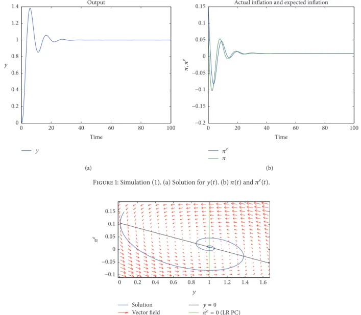
The first simulation, which uses the default parameter values in the program, depicts the transition dynamics for the solution when the equilibrium is a stable focus. The param-eters used are𝑐0 = 10; 𝑖0 = 5; 𝐺 = 5; 𝑏 = 0.8; 𝑘 = 0.05; 𝑑 = 0.05; ℎ = 0.1; 𝜏 = 0.3; 𝛼 = 0.1; 𝛽 = 1; ̇𝑚 = 0.01; 𝑦𝑛=
1. The initial conditions are 𝑦(𝑡0) = 0.05 and 𝜋𝑒(𝑡0) = 0.15,
where𝑡0= 0 is the initial time.
We have 1/𝑑 > 𝛽; hence the steady state (𝑦∗, 𝜋𝑒∗) = (𝑦𝑛, ̇𝑚) is stable, as we can see from Figure 1. Also, the solutions are clearly oscillating. One can check that actual inflation oscillates more than the expected inflation and, naturally, the latter follows the first in its adjustment. Figure 2 illustrates the phase diagram which depicts the stable spiral.
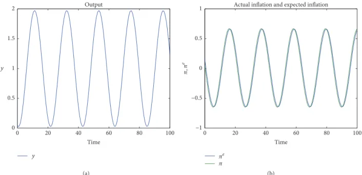
The second simulation presents a different dynamic adjustment. We set𝑑 = 0.5 and 𝛽 = 2, all other parameter values remaining equal. Since1/𝑑 = 𝛽 the equilibrium is now a stable centre. The evolution of output and expected and actual inflation and the phase diagram are depicted in Figures 3 and 4, respectively.
Both figures show that there is no convergence or diver-gence towards the steady state, as the latter is only stable in the Lyapunov sense. All solutions are periodic orbits with period 𝑇 = 2𝜋/𝜔, where 𝜔 is the imaginary part of the corresponding complex eigenvalues.
Output y 20 40 60 80 100 0 Time 0 0.2 0.4 0.6 0.8 1 1.2 1.4 y (a)
Actual inflation and expected inflation
e −0.2 −0.15 −0.1 −0.05 0 0.05 0.1 0.15 , e 20 40 60 80 100 0 Time (b)
Figure 1: Simulation(1). (a) Solution for 𝑦(𝑡). (b) 𝜋(𝑡) and 𝜋𝑒(𝑡).
0.2 0.4 0.6 0.8 1 1.2 1.4 1.6 0 y −0.1 −0.05 0 0.05 0.1 0.15 e Solution Vector field ̇y = 0 ̇ e= 0 (LR PC)
Figure 2: Simulation(1). Phase diagram depicts a stable focus.
Figure 4 presents no ̇𝑦 = 0 locus, since its slope is equal to zero, as we can infer from the analysis in the previous section. For the third simulation, we now set𝑑 = 1 and 𝛽 = 1.2, with all other parameter values equal to the default setup. Inasmuch as𝛽 > 1/𝑑 we know that the equilibrium will be unstable. Moreover, because of this, ̇𝑦 = 0 is negatively sloped. Furthermore, with this set of parameters, the equilib-rium can be shown to be an unstable focus (recall also that𝛼 is very low), so the solution oscillates away from the steady state. This is confirmed by Figures 5 and 6.
Once again, we can see that expected inflation follows up closely after actual inflation, reflecting the way by which expectations are formed.
In the fourth simulation we set𝑑 = 0.025 and dramati-cally decrease𝛽 to 0.1. Now the eigenvalues are real and, since 1/𝑑 > 𝛽, the equilibrium is a stable node.
By inspection of Figure 7 one can observe that, contrary to the previous cases, expectations are now formed correctly,
as expected inflation now decreases steadily towards the steady state level, whereas actual inflation overshoots its equilibrium level, following the evolution of real output.
Figure 8 shows the phase diagram where we can observe that the steady state is a stable node in the fourth simulation.
Remark 4. The parametrization required for the equilibrium
to become an unstable node seems implausible as it imposes either exceedingly high values for 𝛼 or implies trajectories assuming negative values for output. Therefore, we rule out this possibility.
4. Modeling Shocks
In this section we introduce three different types of shocks to the dynamic AS-AD model. A combination between any of the shocks is possible, but for the sake of presentation we simulate each separately and report the results. The baseline
Output 20 40 60 80 100 0 Time 0 0.5 1 1.5 2 y y (a)
Actual inflation and expected inflation
20 40 60 80 100 0 Time −1 −0.5 0 0.5 1 , e e (b)
Figure 3: Simulation(2). (a) Solution for 𝑦(𝑡). (b) Solutions for 𝜋(𝑡) and 𝜋𝑒(𝑡).
0.5 1 1.5 2 0 y −0.8 −0.6 −0.4 −0.2 0 0.2 0.4 0.6 0.8 e Solution Vector field ̇y = 0 ̇ e= 0 (LR PC)
Figure 4: Simulation(2). Phase diagram shows that the equilibrium is a stable centre.
set for parameter values presented here is the same across all simulations and is equal to the default (first) setup presented in Section 3.
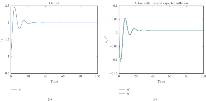
First, we run an expansionary fiscal policy shock, setting new values for public spending and the tax rate at𝐺 = 5.5 and 𝜏 = 0.25, respectively, after the program asks for the implementation of policy shocks. Previous to the shock, the economy is at equilibrium with𝜋 = 𝜋𝑒 = 0.01 and 𝑦 = 1. After a permanent increase in the government spending and permanent decrease in the tax rate at the initial time𝑡0, the economy must jump up to a higher level output. This is given by the AD curve in (8). At𝑡0, real output𝑦 jumps to a new level 𝑦0 = 2.0799 (this result is given by the new initial condition 𝑦0 from the output in the command window from Matlab. See Appendix B.2 for more details). The eco-nomy is now further away from its equilibrium level. Since the level of natural output is unchanged, the economy will
converge to its initial equilibrium level and will do so in an oscillatory fashion, after a very sharp decrease in output in the first periods. Conversely, inflation increases sharply after𝑡0 (however, it does not change at𝑡0) but then starts to converge to its initial value, also oscillating. This situation is described in Figure 9.
The ̇𝜋𝑒 = 0 and ̇𝑦 = 0 loci are unaffected after the shock and the steady state lie at their intersection. Figure 10 shows the phase diagram, with the economy slowly returning to the steady state after its deviation at𝑡0 due to the fiscal policy shock.
The second shock is an expansionary monetary policy shock. We set the money supply growth rate𝑚 = 0.04 oncė the function asks to set new parameter values. Once again, previous to the shock, the economy is at equilibrium with 𝑦 = 𝑦𝑛= 1 and 𝜋𝑒= 𝜋 = ̇𝑚 = 0.01. After the shock occurring
Output y 20 40 60 80 100 0 Time −0.5 0 0.5 1 1.5 2 2.5 y (a)
Actual inflation and expected inflation
e 20 40 60 80 100 0 Time −1 −0.5 0 0.5 1 , e (b)
Figure 5: Simulation(3). (a) Solution for 𝑦(𝑡). (b) Solutions for 𝜋(𝑡) and 𝜋𝑒(𝑡).
Solution Vector field ̇y = 0 ̇ e= 0 (LR PC) −1 −0.8 −0.6 −0.4 −0.20 0.2 0.4 0.6 0.81 e 0.5 1 1.5 2 2.5 0 y
Figure 6: Simulation(3). Phase diagram illustrates an unstable focus.
is out of equilibrium and will oscillate towards the new steady state, where𝑦 = 1 and 𝜋𝑒= 0.04. This situation is reported in Figure 11.
Initially, output will rise as will inflation. After𝑦 crosses the ̇𝑦 = 0 locus, it will start to decrease while inflation continues to rise. Only when the solution crosses the𝜋𝑒̇ = 0 locus will inflation start to fall. At this point, expected inflation will lie above its steady state value and output will be lower than𝑦𝑛. The oscillating process continues as output converges to its natural level𝑦𝑛= 1 and expected and actual inflation converge to their new equilibrium value𝑚 = 0.04.̇ This process is illustrated in Figure 12.
The third and final shock we consider is a supply side shock. It is given by a positive technological shock which, for exogenous reasons, affects the natural level of output, such that 𝑦𝑛 = 2. At the time of the shock, both ̇𝜋𝑒 = 0 and ̇𝑦 = 0 loci shift rightwards, which is straightforward from (12) and (11). Hence, the economy will adjust towards the new
steady state given by the intersection between the two new curves. Since the growth rate of money supply is unchanged, we can anticipate that the steady state levels of actual and expected inflation are the same and given by𝜋 = 𝜋𝑒 = 0.01. However, real output at the new steady state is now given by 𝑦 = 𝑦𝑛= 2. Again, convergence towards the new equilibrium is oscillatory, with a decrease in both actual and expected inflation and an increase in real output in the first periods. This case is depicted in Figures 13 and 14.
5. Concluding Remarks
We studied the dynamic properties of a simple dynamic version of the well known AD-AS model and used code, embedded in a single Matlab function, to simulate the model in order to numerically analyse the dynamic adjustments in the economy under a wide array of different applications concerning policy shocks.
Output 0 0.2 0.4 0.6 0.8 1 1.2 1.4 y 20 40 60 80 100 0 Time y (a)
Actual inflation and expected inflation
−0.02 0 0.02 0.04 0.06 0.08 0.1 0.12 , e 20 40 60 80 100 0 Time e (b)
Figure 7: Simulation(4). (a) Solution for 𝑦(𝑡). (b) Solutions for 𝜋(𝑡) and 𝜋𝑒(𝑡).
0.4 0.6 0.8 1 1.2 0.2 y 0.02 0.04 0.06 0.08 0.1 0.12 0.14 e Solution Vector field ̇y = 0 ̇ e= 0 (LR PC)
Figure 8: Simulation(4). Phase diagram illustrates a stable node.
By standard analytical inspection of the linearised system of the resulting two differential equations, we find that the inflation model may have either stable or unstable spirals (focuses), or nodes, but no saddle point equilibria. Unstable nodes are ruled out numerically. A degenerate Hopf bifur-cation occurs when the value of the demand for money balance’s sensitivity to variations in the nominal interest rate is inversely proportional to the way expectations on inflation are formed, which explains the smooth transition between unstable and stable focuses. However, the model’s linearity naturally rules out any possibility for occurrence of limit cycles.
Numerical simulations of the model with recurrence to the function developed in Matlab allow for the illustration of different cases of dynamic adjustments, with a complete description of the results. Furthermore, the function conve-niently accounts for the possibility of implementing different shocks after the initial simulation. These shocks pertain to
monetary and fiscal policy shocks and supply side shocks. The function also shows how the transition to new steady state levels may occur, with appropriate illustrations and output.
One of our goals is to motivate researchers both within and outside the economics profession for the prospec-tive complementarity in both analytical and numerical approaches. Shunning away computer simulations for the sake of closed form solution and elegant mathematics may preclude tackling more realistic settings, or otherwise intractable. This could thwart possible theoretical and empir-ical contributions that are potentially relevant for policy makers.
Admittedly, the AD-AS model is oversimplifying in its assumptions and limited in accounting for complex business cycles and other economic phenomena. We do not see this as a contradiction in our goals, nor does it defeat our purposes. For instance, further extensions of this simple setup could build theoretical improvements based on microfoundations
Output y 0.5 1 1.5 2 2.5 y 20 40 60 80 100 0 Time (a)
Actual inflation and expected inflation
e −0.05 0 0.05 0.1 0.15 0.2 , e 20 40 60 80 100 0 Time (b)
Figure 9: Fiscal policy shock. (a) Solution for𝑦(𝑡). (b) Solutions for 𝜋(𝑡) and 𝜋𝑒(𝑡).
1 1.5 2 2.5 3 0.5 y −0.05 0 0.05 0.1 0.15 0.2 e Solution Vector field ̇y = 0 (2) ̇y = 0 (1) ̇ e= 0 (LR PC) (1) ̇ e= 0 (LR PC) (2)
Figure 10: Phase diagram portraying the dynamic adjustment after a fiscal policy shock.
for Keynesian aggregate demand and aggregate supply such as in Farmer [24]. Other possible developments would include incorporating technological changes and determine their impact on economic growth rates, following works such as Dutt [25].
It is in our view, however, that the simplicity and percep-tiveness of the AS-AD model studied here allows us to better convey our message and thus contributes to further connect the bridge between economic models’ analytical results and computer based numerical simulations.
Appendix
A. Proof of Proposition 3
Here we provide the full analytical proof that the AD-AS model undergoes a Hopf bifurcation at𝑑 = 𝑑0.
Proof of Proposition 3. Let𝜆𝑗= V(𝑑)±𝑖𝜔(𝑑) ∈ C2, 𝑗 = {1, 2},
denote the pair of eigenvalues obtained from the Jacobian matrix in (20), where 𝑑 is the bifurcation parameter. The conditions for existence of a Hopf bifurcation [26], [27, Th. 3.4.2 in p. 151] are given by
(i)𝜔(𝑑0) ̸= 0; (ii)V(𝑑0) = 0; (iii)V(𝑑0) ̸= 0.
When𝑑 = 𝑑0 = 1/𝛽, the condition for existence of complex eigenvalues in (22) is satisfied, since4𝛽2 > 0. Therefore, we have 𝜔(𝑑0) ̸= 0, which satisfies condition (i). Next, V(𝑑0) gives us the trace of the Jacobian matrix, tr(𝐽), evaluated at the bifurcation point𝑑0= 1/𝛽. This yields
V (𝑑0) = −𝛼 [1 − 𝑏 (1 − 𝜏) + 𝑏𝑘/𝑑ℎ (𝛽 − 𝛽) ] = 0, (A.1)
Output 0.95 1 1.05 1.1 1.15 1.2 1.25 y 20 40 60 80 100 0 Time y (a)
Actual inflation and expected inflation
0.01 0.02 0.03 0.04 0.05 0.06 , e 20 40 60 80 100 0 Time e (b)
Figure 11: Monetary policy shock. (a) Solution for𝑦(𝑡). (b) Solutions for 𝜋(𝑡) and 𝜋𝑒(𝑡).
0.8 0.9 1 1.1 1.2 1.3 1.4 1.5 1.6 0.7 y 0.01 0.02 0.03 0.04 0.05 0.06 0.07 0.08 e Solution Vector field ̇y = 0 (2) ̇y = 0 (1) ̇ e= 0 (LR PC) (1) ̇ e= 0 (LR PC) (2)
Figure 12: Phase diagram portraying the dynamic adjustment after a monetary policy shock.
Finally, taking the first-order derivative ofV(𝑑), we get V(𝑑) = 𝛼ℎ [𝑏 (𝛽𝑘 + 𝜏 − 1) + 1]
{𝑑 [𝑏 (𝜏 − 1) + 1] + 𝑏𝑘}2. (A.2) Evaluating at𝑑0= 1/𝛽 yields
V(𝑑0) = 𝛼𝛽2ℎ
𝑏 (𝛽𝑘 + 𝜏 − 1) + 1 ̸= 0. (A.3) Hence, condition (iii) holds and the model undergoes a Hopf bifurcation at𝑑 = 𝑑0. The additional genericity condition
that the first Lyapunov exponent is nonzero, [28] [27, Th. 3.4.2 (H2) p. 151] is as follows: 𝑎 = 1 16(𝑓𝑥𝑥𝑥+ 𝑓𝑥𝑦𝑦+ 𝑔𝑥𝑥𝑦+ 𝑔𝑦𝑦𝑦) +16𝜔1 [𝑓𝑥𝑦(𝑓𝑥𝑥+ 𝑓𝑦𝑦) − 𝑔𝑥𝑦(𝑔𝑥𝑥+ 𝑔𝑦𝑦) − 𝑓𝑥𝑥𝑔𝑥𝑥+ 𝑓𝑦𝑦𝑔𝑦𝑦] , (A.4)
where𝑎 is the first Lyapunov exponent, 𝑓 = ̇𝑦, and 𝑔 = ̇𝜋𝑒in (13) and subscripts denoting different order derivatives eval-uated at equilibrium and at𝑑 = 𝑑0. Since all the derivatives
Output y 0.5 1 1.5 2 2.5 y 20 40 60 80 100 0 Time (a)
Actual inflation and expected inflation
e 20 40 60 80 100 0 Time −0.15 −0.1 −0.05 0 0.05 0.1 , e (b)
Figure 13: Supply side shock. (a) Solution for𝑦(𝑡). (b) Solutions for 𝜋(𝑡) and 𝜋𝑒(𝑡).
1.5 2 2.5 3 3.5 1 y −0.15 −0.1 −0.05 0 0.05 0.1 e Solution Vector field ̇y = 0 (2) ̇y = 0 (1) ̇ e= 0 (LR PC) (1) ̇ e= 0 (LR PC) (2)
Figure 14: Phase diagram portraying the dynamic adjustment after a supply side shock.
of order higher or equal to 2 are zero, we have𝑎 = 0. There-fore, no periodic solutions exist for𝑑 ̸= 𝑑0, and the bifurca-tion is degenerate, which concludes the proof.
B. Matlab’s Output in Command Window
In this Appendix we provide the Matlab function’s reports on some of the simulations and shocks exemplified in the previous sections.B.1. Output for First Simulation. The first example is given
after the first simulation, using the default parameter values set by the program (see Section 3) (See Box 1).
B.2. Output for First Shock. After the expansionary fiscal
shock (recall Section 4), the function’s reported output in Matlab’s command window was as in Box 2.
Disclosure
Part of this work was developed while Jos´e M. Gaspar was a Ph.D. student at the School of Economics and Management, University of Porto.
Conflicts of Interest
AS-AD dynamic model: dy/dt=a1*dm/dt-alpha(a1-a2*beta)*(y-yn)-a1*pie dpie/dt=beta*alpha(y-yn)
AS and AD curves: (AD) y=dm/dt-alpha(a1-a2*beta*pie (Long run AS) y=yn y: Real output
pie: Expected inflation
a0=(c0+i0+G)/(1-b*(1-tau)+((h*k)/d) = 37.037 a1:(h/d)/(1-b*(1-tau)+((h*k)/d)) = 3.7037 a2: h/(1-b*(1-tau)+((h*k)/d)) = 0.185185
Parameter values: c0 = 10; i0 = 5; G = 5; b = 0.8; k = 0.05; d = 0.05; h = 0.1; tau = 0.3; alpha = 0.1; beta = 1; mdot = 0.01; yn = 1;
Initial conditions: y0 = 0.05; pie0 = 0.15
-Steady-State:
Steady-state real ouput Steady state expected inflation
1.000000 0.010000
Steady state actual inflation 0.0100
Eigenvalues
−0.1759 + 0.5826i −0.1759 - 0.5826i
Stable spiral.
Box 1: Dynamic AS-AD model.
a0 = 41 a1 = 4 a2 = 0.2
New parameter values: c0 = 10; i 0 = 5; G = 5.5; b = 0.8; k = 0.05; d = 0.05; h = 0.1; tau = 0.25; alpha = 0.1; beta = 1; mdot = 0.01; yn = 1;
New initial conditions: y0 = 2.07998; pie0 = 0.0100036
-New Steady-State:
Steady-state real ouput Steady state expectedinflation
1.000000 0.010000
Steady state actual inflation 0.0100
Box 2: Policy and technology shocks.
Acknowledgments
The author thanks ´Oscar Afonso and Paulo B. Vasconcelos for very useful comments and suggestions. Jos´e M. Gaspar gratefully acknowledges support from CEF.UP. This research was financed by the European Regional Development Fund through COMPETE 2020, Programa Operacional Compet-itividade e Internacionalizac¸˜ao (POCI), and by Portuguese Public Funds through Fundac¸˜ao para a Ciˆencia e Tecnolo-gia in the framework of the project POCI-01-0145-FEDER-006890 and the Ph.D. scholarship SFRH/BD/90953/2012.
Supplementary Materials
The Matlab code is embedded in a single function (ADAS-dynamic.m). Add the “.m” file to the working Matlab path/directory. Open Matlab and run the name of the file in the command window (ADASdynamic). The programme asks the user to introduce values for the parameters described
throughout the paper, including the initial time and final time. It then produces three figures and one for the solution 𝑦(𝑡), another for both 𝜋𝑒(𝑡) and 𝜋(𝑡), and the last one shows the phase diagram portraying the transition dynam-ics. The programme will then ask the user to implement either monetary, fiscal, supply side shocks, or any possible combination of shocks, by introducing new values for the money growth rate, public spending, tax rate, and level of natural output. This will produce three new graphs, with the same information as described previously, but compared to the initial situation. Therefore, the figures shown after imple-menting shocks will portray the global transition dynamics towards the new equilibrium. Along these processes, the output for the relevant steady state levels and their qualitative properties are shown in Matlab’s command window, along with the parameter values. See Appendix B for an example of how the output is displayed in Matlab’s command window.
References
[1] A. Lehtinen and J. Kuorikoski, “Computing the perfect model: Why do economists shun simulation?” Philosophy of Science, vol. 74, no. 3, pp. 304–329, 2007.
[2] E. Yavari and T. Roeder, “Model enrichment: Concept, measure-ment, and application,” Journal of Simulation, vol. 6, no. 2, pp. 125–140, 2012.
[3] C. M. Macal and M. J. North, “Tutorial on agent-based mod-elling and simulation,” Journal of Simulation, vol. 4, no. 3, pp. 151–162, 2010.
[4] C. M. Macal and M. J. North, “Successful approaches for teach-ing agent-based simulation,” Journal of Simulation, vol. 7, no. 1, pp. 1–11, 2013.
[5] C. M. Macal, “Everything you need to know about agent-based modelling and simulation,” Journal of Simulation, vol. 10, no. 2, pp. 144–156, 2016.
[6] R. M. Goodwin, “The nonlinear accelerator and the persistence of business cycles,” Econometrica, vol. 19, no. 1, p. 1, 1951. [7] V. Torre, “Existence of limit cycles and control in complete
Keynesian system by theory of bifurcations,” Econometrica, vol. 45, no. 6, pp. 1457–1466, 1977.
[8] W. W. Chang and D. J. Smyth, “The existence and persistence of cycles in a non-linear model: Kaldor’s 1940 model re-examined,”
The Review of Economic Studies, vol. 38, no. 1, pp. 37–44, 1971.
[9] N. H. Barbosa-Filho and L. Taylor, “Distributive and demand cycles in the US economy—A structuralist Goodwin model,”
Metroeconomica, vol. 57, no. 3, pp. 389–411, 2006.
[10] A. C.-L. Chian, E. L. Rempel, and C. Rogers, “Complex eco-nomic dynamics: Chaotic saddle, crisis and intermittency,”
Chaos, Solitons & Fractals, vol. 29, no. 5, pp. 1194–1218, 2006.
[11] Z. Wang, X. Huang, and G. D. Shi, “Analysis of nonlinear dynamics and chaos in a fractional order financial system with time delay,” Computers & Mathematics with Applications, vol. 62, no. 3, pp. 1531–1539, 2011.
[12] C. Bianca, M. Ferrara, and L. Guerrini, “The time delays’ effects on the qualitative behavior of an economic growth model,”
Abstract and Applied Analysis, vol. 2013, Article ID 901014, 2013.
[13] L. De Cesare and M. Sportelli, “A dynamic IS-LM model with delayed taxation revenues,” Chaos, Solitons & Fractals, vol. 25, no. 1, pp. 233–244, 2005.
[14] M. Neamtu, D. Opris, and C. Chilarescu, “Hopf bifurcation in a dynamic IS LM model with time delay’,” Chaos Solitons &
Fractals, vol. 34, no. 2, pp. 519–530, 2007.
[15] L. Zhou and Y. Li, “A dynamic IS-LM business cycle model with two time delays in capital accumulation equation,” Journal of
Computational and Applied Mathematics, vol. 228, no. 1, pp. 182–
187, 2009.
[16] M. Sportelli, L. De Cesare, and M. T. Binetti, “A dynamic IS-LM model with two time delays in the public sector,” Applied
Mathematics and Computation, vol. 243, pp. 728–739, 2014.
[17] A. G. Wilson, “Complex spatial systems: challenges for mod-ellers,” Mathematical and Computer Modelling, vol. 36, no. 3, pp. 379–387, 2002.
[18] R. G. Sargent, “Verification and validation of simulation mod-els,” Journal of Simulation, vol. 7, no. 1, pp. 12–24, 2013. [19] R. G. King, C. I. Plosser, and S. T. Rebelo, “Production, Growth
and Business Cycles: Technical Appendix,” Computational
Eco-nomics, vol. 20, no. 1-2, pp. 87–116, 2002.
[20] R. G. King, C. I. Plosser, and S. T. Rebelo, “Production, growth and business cycles. I. The basic neoclassical model,” Journal of
Monetary Economics, vol. 21, no. 2-3, pp. 195–232, 1988.
[21] R. G. King, C. I. Plosser, and S. T. Rebelo, “Production, growth and business cycles. II. New directions,” Journal of Monetary
Economics, vol. 21, no. 2-3, pp. 309–341, 1988.
[22] R. Shone, Economic Dynamics: Phase Diagrams and Their
Eco-nomic Application, Cambridge University Press, Cambridge,
UK, 2nd edition, 2002.
[23] J. Lee, “The robustness of Okun’s law: Evidence from OECD countries,” Journal of Macroeconomics, vol. 22, no. 2, pp. 331– 356, 2000.
[24] R. E. Farmer, “Aggregate demand and supply,” International
Journal of Economic Theory, vol. 4, no. 1, pp. 77–93, 2008.
[25] A. K. Dutt, “Aggregate demand, aggregate supply and economic growth,” International Review of Applied Economics, vol. 20, no. 3, pp. 319–336, 2006.
[26] J. Marsden and M. McCracken, The Hopf Bifurcation and Its
Applications, Springer-Verlag, Heidelberg, Berlin, 1976.
[27] J. Guckenheimer and P. Holmes, Nonlinear Oscillations,
Dynam-ical Systems, and Bifurcation of Vector Fields, Springer-Verlag,
2002.
[28] B. Hassard and Y. H. Wan, “Bifurcation formulae derived from center manifold theory,” Journal of Mathematical Analysis and
Hindawi www.hindawi.com Volume 2018
Mathematics
Journal of Hindawi www.hindawi.com Volume 2018 Mathematical Problems in Engineering Applied Mathematics Hindawi www.hindawi.com Volume 2018Probability and Statistics Hindawi
www.hindawi.com Volume 2018
Hindawi
www.hindawi.com Volume 2018
Mathematical PhysicsAdvances in
Complex Analysis
Journal of Hindawi www.hindawi.com Volume 2018Optimization
Journal of Hindawi www.hindawi.com Volume 2018 Hindawi www.hindawi.com Volume 2018 Engineering Mathematics International Journal of Hindawi www.hindawi.com Volume 2018 Operations Research Journal of Hindawi www.hindawi.com Volume 2018Function Spaces
Abstract and Applied Analysis Hindawi www.hindawi.com Volume 2018 International Journal of Mathematics and Mathematical Sciences Hindawi www.hindawi.com Volume 2018Hindawi Publishing Corporation
http://www.hindawi.com Volume 2013 Hindawi www.hindawi.com
World Journal
Volume 2018 Hindawiwww.hindawi.com Volume 2018Volume 2018