Universidade de Aveiro Departamento de F´ısica, 2016
Diamantino
Castanheira da Silva
Evoluc¸ ˜ao de variedades topol ´
ogicas da perspectiva
das redes complexas
Universidade de Aveiro Departamento de F´ısica, 2016
Diamantino
Castanheira da Silva
Evoluc¸ ˜ao de variedades topol ´
ogicas da perspectiva
das redes complexas
Complex Network View of Evolving Manifolds
de-the jury
Prof. Dr. Manuel Ant ´onio dos Santos Barroso
Professor Auxiliar do Deparamento de F´ısica da Universidade de Aveiro
Prof. Dr. Nuno Miguel Azevedo Machado de Ara ´ujo,
Professor Auxiliar da Faculdade de Ci ˆencias da Universidade de Lisboa (examiner)
Dr. Sergey Dorogovtsev
Universi-acknowledgements Esta tese n ˜ao teria sido poss´ıvel sem o apoio do meu orientador, o pro-fessor Sergey Dorogovtsev e do meu co-orientador Rui Am ´erico. Quero agradecer a todos os colegas do Departamento de F´ısica e em especial aos meus pais, por me apoiarem nesta caminhada.
Abstract Neste estudo investigamos redes complexas formadas por triangulac¸ ˜oes de variedades topol ´ogicas em evoluc¸ ˜ao, localmente homeom ´orficas a um plano. O conjunto de transformac¸ ˜oes dessas redes ´e restringida pela condic¸ ˜ao de que a cada passo todas as faces se mantenham triangulares. Neste trabalho adotamos duas abordagens principais. Na primeira abordagem crescemos variedades usando v ´arias regras simples, que progressivamente adicionam novos tri ˆangulos. Na outra abordagem relaxamos a estrutura de variedades grandes, mantendo o n ´umero de tri ˆangulos constante.
As redes resultantes da evoluc¸ ˜ao destas triangulac¸ ˜oes demontram v ´arias caracter´ısticas interessantes e inesperadas em redes planares, tais como di ˆametros ”small-world” e distribuic¸ ˜oes de grau tipo lei de pot ˆencia. Finalmente manipul ´amos a topologia das variedades pela introduc¸ ˜ao de ”wormholes”. A presenc¸a de ”wormholes” pode mudar a estrutura da rede significamente, dependendo da taxa a que s ˜ao introduzidos. Se introduzirmos ”wormholes” a uma taxa constante, o di ˆametro da rede apresenta um crescimento sub-logar´ıtmico com o n ´umero de nodos do sistema.
We study complex networks formed by triangulations of evolving manifolds, locally homeomorphic to a plane. The set of possible transformations of these networks is restricted by the condition that at each step all the faces must be triangles. We employed two main approaches. In the first approach we grow the manifolds using various simples rules, which pro-gressively had new triangles. In the other approach we relax the structure of large manifolds while keeping the number of triangles constant.
The networks resulting from these evolving triangulations demonstrate several interesting features, unexpected in planar networks, such as small-world diameters and power-law degree distributions.
Finally, we manipulate the topology of the manifolds by introducing worm-holes. The presence of wormholes can change significantly the network structure, depending on the rate at which they are introduced. Remarkably,
Contents
Contents i
List of Figures iii
List of Tables v
1 Introduction 1
1.1 Motivation and structure . . . 1
1.2 Related work . . . 2
2 Basic notions 3 2.1 Network basics . . . 3
2.2 Ensemble approach . . . 3
2.3 Reference network models . . . 4
2.4 Simplexes and Manifolds . . . 5
2.5 Object of work . . . 5
2.6 Relations between simplexes . . . 6
3 Rules 7 3.1 Common definitions and procedures . . . 7
3.2 Rules for growth . . . 9
3.3 Variations of rule G3 . . . 10
3.4 Rules for relaxation . . . 11
3.5 Reduction to fundamental rules . . . 12
3.6 n-dimensional rules . . . 14
3.7 Rules table . . . 16
4 Results 19 4.1 Initial results . . . 19
4.2 Experimental method . . . 20
4.3 Rules for growth . . . 20
4.4 Variations of rule G3 . . . 26
4.5 Rules for relaxation . . . 29
5 Evolution of surface topology 33
5.1 Results . . . 34
5.1.1 Fixed number of wormholes . . . 34
5.1.2 Dynamic wormhole introduction . . . 35
5.1.3 General observations . . . 37
6 Methods and characteristics 39 6.1 Statistics . . . 39
6.2 Hausdorff dimensionality . . . 40
6.2.1 Relation between Hausdorff dimension and average distance . . . 40
6.3 Spectral dimension . . . 41
6.4 Pearson Coefficient . . . 42
6.5 Master equations and mean field theory . . . 42
6.6 Fitting methods . . . 43
6.7 Topology evolution methods . . . 43
6.8 Initial surfaces . . . 44
6.9 Computational running costs . . . 45
7 Conclusion 47
Bibliography 49
List of Figures
2.1 Ensemble example . . . 4
3.1 Order of neighbours around a vertex. . . 7
3.2 Expansion and contraction operations . . . 8
3.3 Flip operation diagram. . . 9
3.4 Rule G1 diagram. . . 9
3.5 Rule G2 diagram. . . 9
3.6 Rule R1 diagram. . . 12
3.7 Algorithm G1 emulated by the expansion operation . . . 13
3.8 Algorithm G2 emulated by the expansion operation . . . 13
3.9 Algorithm R1 emulated by the expansion and contraction operations. . . 14
3.10 Algorithm R2 emulated by the expansion and contraction operations. . . 14
3.11 Rule G1 (n = 3) diagram. . . 15
3.12 Rule G2 (n = 3) diagram. . . 15
4.1 Rule G1. Degree distribution. . . 21
4.2 Rule G1. Average distance and Pearson coefficient evolution. . . 22
4.3 Rule G2. Degree distribution and average distance evolution. . . 23
4.4 Rules for growing. Exponent of average distance and Pearson coefficient evolution for various rules. . . 25
4.5 Rule G3.1. Hausdorff dimension. . . 26
4.6 Rule G3.2. Hausdorff dimension. . . 27
4.7 Variations of G3. Hausdorff dimension for various rules. . . 28
4.8 Variations of G3. Maximum Hausdorff dimension for various rules. . . 28
4.9 Rule G2. Network characteristics evolution with time. . . 29
4.10 Rule R2. Evolution of time of minimum distance and time of start of equilibrium. . 30
4.11 Rules for relaxation. Average distance and Pearson coefficient evolution with time for various rules. . . 31
5.1 Fixed number of wormholes. Degree Distribution. . . 34
5.2 Fixed number of wormholes (H = 4096). Degree Distribution . . . 35
5.3 Logarithmic dynamic wormhole introduction. Degree distribution. . . 35
5.4 Logarithmic dynamic wormhole introduction. Mean distance. . . 36
5.5 Linear dynamic wormhole introduction. Degree distribution. . . 36
5.6 Linear dynamic wormhole introduction. Mean distance. . . 37
6.2 A ”donut” and a initial surface made of connected donuts. . . 44 6.3 Stages of subdivision of an icosahedron (icosphere). . . 44
List of Tables
3.1 Rules for growth description. . . 16
3.2 Rule G3 variations description. . . 17
3.3 Rules for relaxation description. . . 18
4.1 Rules for growth. Simulation results. . . 25
4.2 Variations of rule G3. Simulation results. . . 28
Chapter 1
Introduction
1.1
Motivation and structure
Network theory has been successful in describing a series of phenomena in various systems such as social, biological or technological systems. Important models have been developed in the last decades, such as the Erd ˝os-R ´enyi model [1] in the late 1950s, the Watts-Strogatz model [2] and the Barabasi-Albert (BA) model [3] [4] in the late nineties, which were fundamental to understand various aspects of complex networks.
However, in recent years there has been a new interest about the geometrical characterization of networks, which these important models did not address. This is an important aspect for various real networks such as transportation networks, communication networks or even the brain, which structure depends on the space in which it is embedded.[5]
This new perspective about networks has been used to study routing problems in the Internet [6, 7, 8], data mining and community detection [9, 10, 11]. The study of properties such as cur-vature and hiperbolicity can be used to determine metrics of networks embedded in a physical space [12, 5], with technological applications such as wireless networks [13].
Even in the field of quantum gravity, there are studies using pre-geometric models, were space is an emergent property of a network of a simplicial complex [14, 15, 16, 17] , which are structures formed by gluing together simplices such as triangles, tetrahedra, etc.
The objective of this work is the study of 2D evolving manifolds, using methods from network theory. The evolution of these manifolds will be made by a set of rules that obey various topo-logical constraints, in order to observe several characteristics, such as degree distribution and average distance of the embedded network.
This document starts by giving a basic introduction to complex network theory and topology (chapter 2). In chapter 3, we present our approach to this problem and introduce the rules used to evolve the manifolds. In chapter 4, we present the results of the simulated networks, discussed them and derive some analytical results. In chapter 5, we extend the model in order to observe the evolution of manifolds by changing their topological properties, consisting on the introduction of wormholes. The last chapter, chapter 6, is a reference to all the methods and characteristics used in this work.
1.2
Related work
The theme of space and networks has been approached from various perspectives by many authors. They explored several aspects, ranging from the discovery of embedded metrics in communication networks [8], to the routing problem in several types of network [7] or even the emergence of geometric and statistical characteristics using networks randomly built from merg-ing simplexes1[18] [19].
The following works [18] [19].
done by Bianconi et al. were a starting point to our present work.
In one of these works [18], the network model was constructed by adding simplexes of dimension
dto the network, building a simplicial complex2. δ-faces (δ < d) were defined as the simplexes of dimensionδ belonging to eachd-simplex, and the generalized degree of aδ-face was defined as the number ofd-simplexes incident to it.
Each (d-1)-face of ad-simplex can be shared by 2d-simplexes at most, so each newd-simplex can only connect to another simplex if it has some (d-1) face not belonging to 2 d-simplexes. Every vertex of eachd-simplex is generated with a random energy value. When a new simplex is introduced, it will connect to a random (n-1)-face, with probability proportional to the energy3 of that face (see preferencial attachment at section 2.3).
The simulation results showed that the average of the generalized degree of theδ-faces forming the simplicial complex can either follow Fermi-Dirac, Boltzmann or Bose-Einstein distributions, depending on the dimension of theδ-faces and of thed-simplexes.
A more simple model [19], was also developed by Bianconi et al., focused in the emergence of curvature in the construction of surfaces based in triangles. Here curvature (Ri) is related to the number of adjacent triangles (ti) to each vertexi, asRi= 1 − ti/6. Although curvature is not a priority in our work, the method developed in this work to evolve a surface is quite interesting. This model has two parametersm, which is the maximum number of triangles connected to an edge, andp, which is a continuous control parameter.
To build such surfaces, they started with just a triangle and then at successive steps used a combination of two processes. The main process is executed in every step, adding a triangle to an random edge which has less thanmtriangles attached to it. An additional process is executed with probability p, consisting in the connection of vertices at distance 2 from each other. This process will only choose two vertices such that each of the two edges between them have less thenmadjacent triangles.
By using different combinations of the two parameters, it was possible to generate ”complex network geometries with non-trivial distribution of curvatures, combining exponential growth and small-world properties”, such as a very slow growth of distance between vertices relative to the number of vertices (see section 2.3).
1
Simplexes ofndimensions are full connected networks ofn + 1vertices.
2A simplicial complex is a set of simplexes in which any face of these simplexes also belongs to the simplicial
complex. A face of a simplex is a simplex of lower dimensionality, belonging to it.
3
Here energy of aδ-face is defined as the sum of the energies of all it’s vertices.
Chapter 2
Basic notions
2.1
Network basics
A network, G, also known as a graph, can be mathematically described as a collection of verticesG(N )and edgesG(E). Each edge is simply the connection between two vertices of the network.
A network can be fully represented by its adjacency matrixaij, in whichaij will be equal to the number of edges fromitoj. Normallyaij will have values0(disconnected) or1(connected by a single edge). A graph can be directed or undirected. A directed graph can have edges that only permit transitions from a vertexvitovj but not fromvj tovi(aij 6= aji). When both directions are permitted for all edges, a graph is called undirected (aij = aji).
In this work, we will only use undirected networks, therefore, the degree of a vertex will be equal to the number of links incident to it. Using the adjacency matrix, the node’s degree calculation is simply: ki = N X j=1 aij (2.1)
in whichN is the number of vertices of the network.
2.2
Ensemble approach
The approach we are using in this work will focus on random networks which are not single networks but a statistical ensemble [20]. The statistical ensemble is defined as a set of particular networks in which each one of them has a given probability of realization. In this work, each ensemble will be formed by networks grown by a set a rules, that begin with the same initial conditions and have the same number of evolution steps. A clearer definition of this process will be discussed in chapter 3.
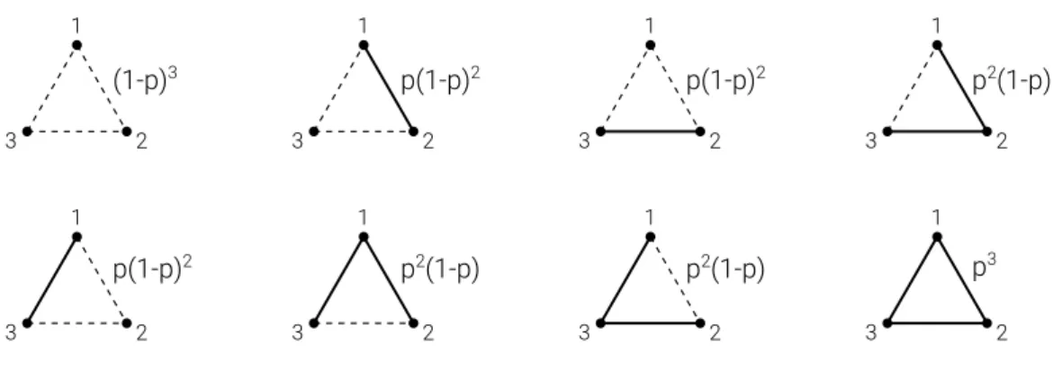
In order to obtain statistics of a certain rule, we will not use the properties of single realization, but the expected characteristics of the possible realizations of this type network, taking into account the realization probability. To illustrate this approach, let us use a small random network composed of exactly 3 nodes. Each possible link can exist independently with probabilityp, so each member of this ensemble will have an existence probability as depicted in figure 2.1.
1 2 3 1 2 3 1 2 3 1 2 3 1 2 3 1 2 3 1 2 3 1 2 3 (1-p)3 p(1-p)2 p(1-p)2 p(1-p)2 p2(1-p) p2(1-p) p2(1-p) p3
Figure 2.1: Ensemble example.
The probability of each member of the ensemble is shown near it.
The degree distribution P (k)in a network will be equal to the expected fraction of vertices with degree equal tok. It is defined as:
P (k) = hN (k)i
N (2.2)
in whichhN (k)iis the average number of vertices with degreek, averaged over all the members of the ensemble and N is the number of vertexes. Therefore, the nth moment of the degree distribution, can be calculated by:
hkni =X
k
P (k)kn (2.3)
A path between vertexiand vertexj is a sequence of vertices beginning iniand ending inj, such that each vertex is connected by an edge to the next vertex. The length of a path is equal to the number of edges in it.
The distance between two nodesiandj,lij, is the minimum length path from vertexito vertexj. This path is called a geodesic. The average distance in a specific networksis the mean distance between all possible pairs of distinct vertices:
hlis= 2 N (N − 1) N X i N X j>i lij (2.4)
Therefore, the average distance in a ensemble, in which a networkshas as weightP (s)is:
hli =X
s
P (s)hlis (2.5)
2.3
Reference network models
To give a better idea of the meaning of the measured quantities, here we present an overview of some basic models and that will serve as a basis of comparison when characterizing our net-works.
The classical random network is built fromN initial nodes. For each distinct pair of nodes, there is a probabilitypof creating a link between them.
The small world network is a kind of network that has some specific characteristics related to average distance. To be small-world, the average distance between vertices should grow loga-rithmically with the system size.
One of the most simple models that manifest this kind of characteristics is the Watts-Strogatz model [2], which starts with a lattice structure forming a ring and with the addition of shortcuts, the network mean distance falls dramatically. In fact, this modification makes the mean distance growth with system size to go from linear to logarithimic.
A very important mechanism for growing networks is the preferential attachment mechanism. One of the first models to demonstrate this mechanism was the Barabasi-Albert model [3, 4], in which a new vertex introduced in the network, connecting tomrandom vertices, given a weight function proportional to its degree. Basically, that mechanism tends to increase the number of connections of the high degree nodes. In fact, the BA-model will converge to a heavy-tail degree distributionP (k) ∼ k−3.
In terms of diameter growth, we can select two networks with very distintic behaviour, lattices and classical random networs. The diameter of an lattice grows with∼ N1/d, in which N is the number of vertexes and dis the number of dimensions. In contrast to this growth, the classical random graph grows with∼ log(N ), which is a slower growth than any lattice.
2.4
Simplexes and Manifolds
A basic building block of topology is then-simplex. A 0-simplex is a point, a 1-simplex is a line, a 2-simplex is a triangle and a 3-simplex is a tetrahedron.
In order to construct more complicated spaces, we can merge faces of various simplexes, ob-taining a simplicial complex. As an example, the surface of a cube can be considered as twelve triangles glued together.
Manifolds are a class of spaces of topology, that near each of its points resembles an-dimensional euclidian space. These manifolds can be resultant, for example, of polynomial or differential equa-tions.
In order to study its global structure, it is helpful to triangulate it, that is, to construct a home-omorphism to a simplicial complex. For example, the surface of a sphere is a 2D manifold, homeomorphic1to a cube. [21]
2.5
Object of work
The manifolds that interest us resemble a 2D euclidian space near each of its points. Some examples of this type of manifolds are a spheres or a torus.
Using triangles, which are 2-simplexes, we can build a simplicial complex that is homeomorphic
1
Homeomorphism is an isomorphism between two topological spaces, in which every point of one topological space can be continuously mapped in the other topological space, in either direction.
to those manifolds. Each edge will be shared between 2 triangles and each triangle will have 3 distinct neighbouring triangles. The resulting simplicial complex will be a surface, from which the nodes and links of the network will be naturally its vertices and edges. We will consider that all edges are undirected.
This object must obey some constraints. Each edge must have only 2 neighbouring triangles and the Euler characteristic (see section 2.6) must be constant if the topology2does not change.
As we will see later (chapter 3) the construction of this object will depend on the chosen rule. It could start from a minimal surface and then be grown or starting with a large surface and then be relaxed.
In contrast with Bianconi’s model [19], in which only edges that were not saturated could evolve, that would lead to the creation of a frozen nucleus and only at the border would be evolution. In our model, every edge, vertex or face is available to evolve.
2.6
Relations between simplexes
Given the properties of our object of work, we can get some basic quantitative relations between the simplexes of the surface. One of the most fundamental equations, that all networks grown in this work will follow, is Euler’s formula:
χ = F + N − E (2.6)
In whichF is the number of faces,N is the number of vertices,E is the number of edges andχ
is the Euler characteristic. χgives us the number of wormholes3,H, this surface has, using the relationχ = 2(1 − H). A sphere hasH = 0, a torus hasH = 1and so on. In closed surfaces, the topology is directly connect toχ, therefore, if the topology of a surface does not change,χmust be constant. Also, when a rule is not changing any number of simplexes of the surface, obviously
χwill not change.
Let us obtain further relations between the simplexes, to see what limitations we have in the simplexe’s evolution. Knowing that each edge has 2 neighbouring triangles and that each triangle has 3 neighbouring edges, we get the relation 3F = 2E. Therefore, the relation between the number of edges and vertices is given by:
N = 1
3E + χ ⇔ E = 3(N − χ) ⇔ F = 2(N − χ) (2.7)
Given the obtained relations between the simplexes in equation 2.7, if we add a single vertex, we need to add 3 edges and 2 faces (triangles). But if we try to add only 1 edge or 1 face, that will create a fraction of a vertex, what is impossible. So, removing or adding a vertex at each step is the minimal evolution we can do.
2We will consider a strict meaning for topology, in which two topological surfaces are equal if they have the same
number of wormholes.
3
See the operative explanation of wormhole in chapter 5.
Chapter 3
Rules
The evolution of the networks that we will study are clearly dependent on the evolution of the surfaces, which will be made in two different approaches, by growing or relaxing these surfaces using very simple rules.
The growth of surfaces starts from a small initial surface, with enough nodes for the rule to op-erate, such a tetrahedron or a octahedron. At each step, the rule introduces 1 new node, 2 new triangles and 3 new edges to the surface. The quantity of introduced simplexes will be the same for any rule, but the way in which these elements are connected to the remaining surface will be what distinguishes each rule.
On the other hand, the rules for relaxation will not change the number of nodes, triangles or edges. The initial surface that they start with must have a considerable number of vertexes, and these rules will just change the structure of this network.
To name these rules, it will be used the letters G (growing) and R (relaxing) followed by a refer-ence number. The list of all used rules can be consulted at the end of this chapter (section 3.7).
3.1
Common definitions and procedures
Before exploring the rules used in this work, some definitions and procedures related to the evolution of a surface must be explained. Many of them will use random choice of elements, and unless otherwise specified, we will assume that this choice is made uniformly.
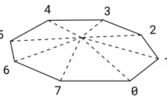
Neighbours order around a vertex
The set of triangles adjacent to a vertex has a border forming a ring, connecting all the neighbour-ing vertices of that vertex. Therefore, if we define a orientation around that rneighbour-ing, we can define a range of neighbours from a neighbour X to neighbour Y.
0 1 2 3 4 5 6 7
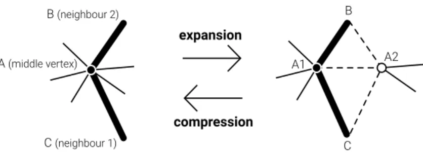
Expansion of a vertex into an edge:
One of the basic operations made to the surface consists in the ”expansion” of a vertex into an edge.
To expand a vertex A, and the two edges that connect to its neighbours B and C, we proceed as follows:
1) Create two new vertices, A1 and A2, and connect them.
2) Connect A1 to the range of neighbours of A from B to C, included. 3) Connect A2 to the range of neighbours of A from C to B, included. 4) Eliminate A.
Contraction of an edge into a vertex:
Another operation consists in the elimination (contraction) of an edge into a vertex, eliminating one vertex.
Let us call vertex A1 and A2 to the ends of a chosen edge, and vertex B and C to the two common neighbors of A1 and A2. The contraction procedure of an edge into a vertex follows the following steps:
1) Eliminate edges A1-A2, B-A2 and C-A2.
2) Connect all remaining neighbors of vertex A2 to vertex A1. 3) Eliminate vertex A2.
A (middle vertex) B (neighbour 2) C (neighbour 1) expansion compression C A2 A1 B
Figure 3.2: Expansion and contraction operations. The thick lines and full vertices represent the selected elements. The dashed lines and empty vertices represent the new elements.
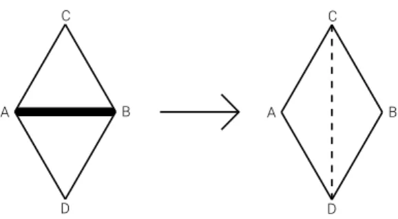
Flip
Given a chosen edge, we will have its two end vertices, A and B and two common neighbours to A and B, let us call them C and D. To make the flip operation, we simply eliminate the edge between A and B and create a new one between C and D.
D C A B D C A B
Figure 3.3: Flip operation diagram.
3.2
Rules for growth
In order to grow a network, we just need to insert a new vertex. A simple way to do that consists in splitting simplexes of the surface. So we started by designing rule G1, that will divide triangles and rule G2 that will divide edges.
Rule G1
This rule will simply introduce a new vertex, by subdividing a triangle in 3 triangles at each step. Schematically, we can represent the evolution steps like this:
Figure 3.4: Rule G1 diagram.
Rule G2
This rule will introduce a new vertex by dividing an edge into two. Given the constraints of our model, all the faces must be triangles, then the two adjacent triangles to the original edge are also divided.
Figure 3.5: Rule G2 diagram.
The main idea of this rule is to choose one sequence of three vertices such that they form a con-nected chain, and then expand the middle vertex, using the expansion mechanism (see the initial part of this chapter and figure 3.2). To do that, a random vertex is chosen an then two neighbours are also chosen at random. This rule make its choices in the most simple and uniform way as possible. No preferential functions are used, just the simple selection of simplexes.
Rule G4
This rule is almost equal to the last one (G3), but it will make a flip after the expansion of the vertex, adding some structural destruction. But not without a price.
There are some limitations in the implementation of this algorithm. When choosing a second neighbour, this cannot be next to the first one. This is so, because they share an edge, and the flipping would create a new edge between them, something that is forbidden in our model. There-fore, using nodes of degree 3 as the middle vertex is forbidden. Because of this limitations, the most simple and uniform initial surface had to be an octahedron, instead of a tetrahedron.
Rule G5
This rule also uses the expansion mechanism, like in rule G3, but makes its choices based on edges, not on vertices. We start by choosing an edge at random, the next edge will be chosen from the set of edges connect to that first edge.
Rule G6
This rule is similar to rule G5, but it simplifies the choice procedure of the new edge. Instead of building a set of all edges connected to the first chosen edge, it just choose one of it’s ends, and then chooses an edge connected to that end.
3.3
Variations of rule G3
Rule G3 follows a very simple procedure, having no functions of preferential choice, simply choos-ing simplexes uniformly at random.
During the implementation of the algorithm that simulated rule G3, we asked ourselves ”what if we change the probabilities of choosing the second neighbour next to the first neighbour?”. So as a first experiment, we reduced it to half of any other neighbour choice. As a consequence of this, the Hausdorff dimension decreased. So, we learned a way of manipulating the dimensionality of this network, by manipulating the way that the neighbours are chosen. Our observations of sec-tion 4.4, suggest that the closer the two chosen neighbours are, the higher will be the dimension. With this insight, we then created rules based in rule G3, but with different choice mechanisms. These new rules will give us information on the impact of these new choices in the characteristics of the network, such as degree distribution, average distance and dimensionality.
Rule G3.1
Inspired by the previous experience, we created a new rule in which we forced the choice of the two neighbours, the most far apart from each other.
With this in mind, we start by choosing the first neighbour at random. Using the ordering of neighbours around the middle vertex (see section 3.1), and assuming that the first neighbour is in positioni, then the choice of the second neighbour will be in positioni ± k/2, if kis even, or we choose betweeni ± (k + 1)/2ori ± (k − 1)/2ifkis odd.
Rule G3.2
In the reverse approach we can try to get the highest dimension possible by choosing the nearest two neighbours.
This rule clearly relates to rule G1, where the two neighbours are chosen in the same way. The difference lies in the middle vertex choice. In the case of algorithm G3.2, the vertex is chosen uniformly, but in the case of algorithm G1, the choice of vertex is proportional to the vertex degree.
Rule G3.3
To test if choosing high degree nodes for the middle vertex, leads to a lower dimensionality, we created this algorithm. The first choice (global) will be an triangle at random. Then the highest degree vertex is chosen as the vertex to expand. The two neighbours are chosen at random.
Rule G3.4
This rule is a variation of the previous rule (G3.3), but instead of a triangle as the first element to be chosen, it will be an edge. The choice for middle vertex, by highest degree rule will be maintained.
Rule G3.5
To simplify the process of choice, this rule simply chooses an edge at random and then chooses one of it’s ends at random. The two neighbours of the middle vertex are also chosen at random. This rule will create a preferential choice for the middle vertex.
Rule G3.6
This rule is almost the same as rule G3.5, but the vertex that will be expanded is the highest degree end of the chosen edge.
3.4
Rules for relaxation
The other set of rules, the rules for relaxation, begin with an already grown network. The main idea of these rules is to modify the network’s structure, keeping the number of simplexes constant, until it reaches an equilibrium state, where the network’s characteristics, such as the average degree distribution, stop evolving. The initial network can be generated by a growing algorithm, or it can use a predefined initial surface (see section 6.8).
In fact, the kind of initial surface is almost irrelevant [20] , assuming that every simplex config-uration for the same number of vertices is reachable from any other configconfig-uration, after many iterations the resulting surface should be independent of the initial one. This holds true for all the rules for relaxation, except for rule R1.
Rule R1
this rule combines rule G1 and another rule that will do the reverse of G1, by removing a node of degree 3. It is obvious that this rule has several limitations. It only works if nodes of degree 3 exist, so the initial surface must be generated by an algorithm that guarantees those kind of vertices, such as a surface evolved by rule G1. There is also the risk of having4-cores1that will not relax. There is also the risk of having so little degree 3 nodes, that they only be relocated from one triangle to another, not changing the structure very much, or taking a huge number of steps to reach equilibrium.
Figure 3.6: Rule R1 diagram.
Rule R2
This simple rule is based in the flipping mechanism presented in section 3.1. At each step, it will flip a random edge from the surface (fig 3.3). It’s main purpose is to shuffle the possible correla-tions between neighbouring vertices.
Rule R3
This rule combines the contraction mechanism and an expansion rule. The expansion rule intro-duces a vertex and the contraction rule removes one vertex. Therefore, the number of simplexes is maintained. In this case, rule G3 was chosen as the expansion rule.
Rule R4
This last rule is just an variation of R3, where rule G4 was used in the expansion, instead of rule G3.
3.5
Reduction to fundamental rules
All the rules that were presented, can be expressed in terms of more fundamental rules. These fundamental rules are based in the ”expansion” and ”contraction” operations. By using them, we can emulate any other rule, being only a matter of finding the right sequence of opera-tions. Some rules will be recreated, to demonstrate this reduction.
Reduction of rule G1
In order to get the same evolution as rule G1, the choice of the three vertices must be made such that they all belong to the same triangle. To do that, we can starting by choosing a triangle at ran-dom, like the original rule, but then we choose one of the vertices at random. The two neighbours obviously will be the two remaining vertices of the chosen triangle.
1k-core is a subgraph of a network in which every member has at leastkneighbours also belonging in thek-core
This procedure will increase the degree of the middle vertex and the two neighbours, and also create a new vertex of degree 3 connected to the all the vertices of the triangle.
Figure 3.7: Algorithm G1 emulated by the expansion operation
Reduction of rule G2
To recreate this rule, we start by choosing an edge uniformly at random, just like in the original procedure (section 3.2 ). Then, one of its ends is chosen at random, as the middle vertex. The 2 neighbours become the 2 common vertices of the chosen edge. With this choice, we just expand the middle vertex.
Figure 3.8: Algorithm G2 emulated by the expansion operation
Reduction of rule R1
The rules of relaxation do not change the number of simplexes in the surface. Therefore, we will need to combine the contraction mechanism with the expansion mechanism. In section (section 3.4) we saw that R1 consists of two phases, one in which a degree 3 vertex is eliminated and a second phase where a degree 3 vertex is inserted, like in rule G1. The reduction of the first phase starts with a choice of a vertex of degree 3. Then we apply the contraction mechanism using as middle vertex, the chosen vertex, and the two neighbours, any of the vertex’s neighbours.
Figure 3.9: Algorithm R1 emulated by the expansion and contraction operations. The final stage of the expansion and the initial stage of the contraction
could not correspond to the same elements.
Reduction of rule R2
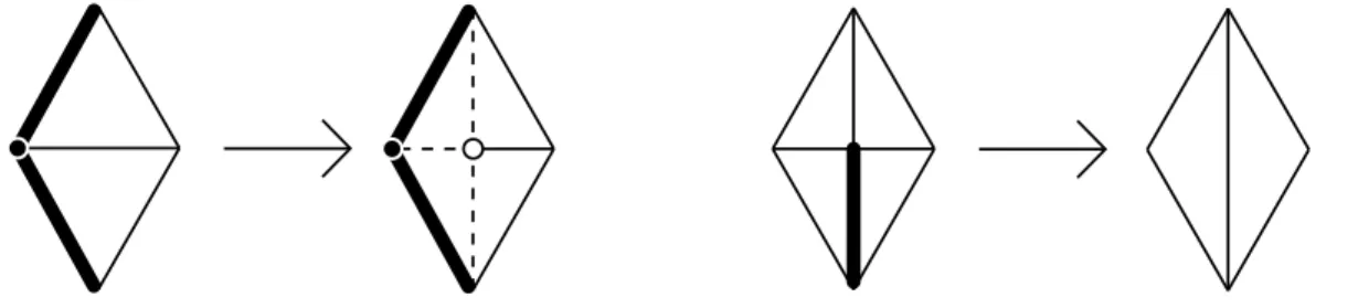
This rule can be also reduced into two stages, a ”expansion” stage and a ”contraction” stage. The first stage is equal to rule G2, where we end up with an extra vertex. In the second stage, the idea is to merge this new vertex with one of two vertices that were initially disconnected, and the flipping is complete.
Figure 3.10: Algorithm R2 emulated by the expansion and contraction operations. The final stage of the expansion and the initial stage of the contraction
must correspond to the same elements.
3.6
n
-dimensional rules
Rules G1 and G2 can be generalized to higher dimensions. Let us suppose that we build a manifold made ofn-simplexes. Each n-simplex hasn + 1 faces (n − 1-simplexes), that can be at most shared by twon-simplexes. The initial geometry is a(n + 1)-simplex, in which each
n-simplex hasn + 1neighbouringn-simplexes.
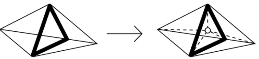
In this setting, G1 can be generalized to an operation that starts by choosing one of the n -simplexes and then connecting a new vertex to all then + 1vertexes of this chosenn-simplex.
Figure 3.11: Rule G1 (n = 3) diagram.
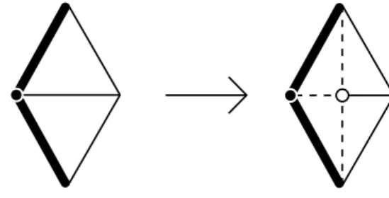
The generalized version of G2 could be thought as an operation that chooses a random face ((n − 1)-simplex) and divides each of the twon-simplexes that share this face inton n-simplexes. In general this consists in connecting a new vertex to all the vertices of the twon-simplexes, but for2-simplexes, we must first eliminate the chosen face (a link).
3.7
Rules table
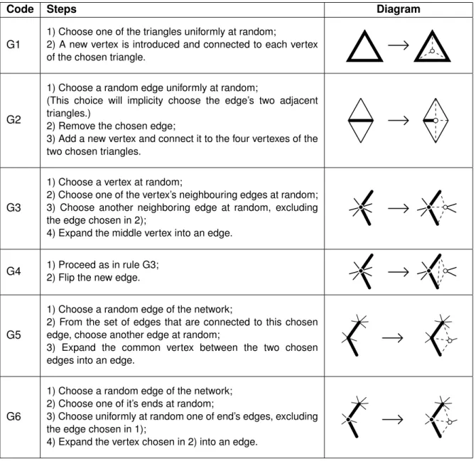
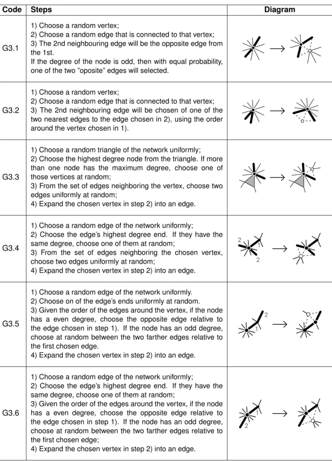
The following tables give a precise description of each rule. The diagrams show selected elements as thick lines and full points, and new geometry as dashed lines and empty points. If a diagram has numbers, they represent the order of selection.
Code Steps Diagram
G1
1) Choose one of the triangles uniformly at random;
2) A new vertex is introduced and connected to each vertex of the chosen triangle.
G2
1) Choose a random edge uniformly at random;
(This choice will implicity choose the edge’s two adjacent triangles.)
2) Remove the chosen edge;
3) Add a new vertex and connect it to the four vertexes of the two chosen triangles.
G3
1) Choose a vertex at random;
2) Choose one of the vertex’s neighbouring edges at random; 3) Choose another neighboring edge at random, excluding the edge chosen in 2);
4) Expand the middle vertex into an edge.
G4 1) Proceed as in rule G3;
2) Flip the new edge.
G5
1) Choose a random edge of the network;
2) From the set of edges that are connected to this chosen edge, choose another edge at random;
3) Expand the common vertex between the two chosen edges into an edge.
G6
1) Choose a random edge of the network; 2) Choose one of it’s ends at random;
3) Choose uniformly at random one of end’s edges, excluding the edge chosen in 1);
4) Expand the vertex chosen in 2) into an edge.
Table 3.1: Rules for growth description.
Code Steps Diagram
G3.1
1) Choose a random vertex;
2) Choose a random edge that is connected to that vertex; 3) The 2nd neighbouring edge will be the opposite edge from the 1st.
If the degree of the node is odd, then with equal probability, one of the two ”oposite” edges will selected.
G3.2
1) Choose a random vertex;
2) Choose a random edge that is connected to that vertex; 3) The 2nd neighbouring edge will be chosen of one of the two nearest edges to the edge chosen in 2), using the order around the vertex chosen in 1).
G3.3
1) Choose a random triangle of the network uniformly; 2) Choose the highest degree node from the triangle. If more than one node has the maximum degree, choose one of those vertices at random;
3) From the set of edges neighboring the vertex, choose two edges uniformly at random;
4) Expand the chosen vertex in step 2) into an edge.
G3.4
1) Choose a random edge of the network uniformly;
2) Choose the edge’s highest degree end. If they have the same degree, choose one of them at random;
3) From the set of edges neighboring the chosen vertex, choose two edges uniformly at random;
4) Expand the chosen vertex in step 2) into an edge.
1 2
2
G3.5
1) Choose a random edge of the network uniformly. 2) Choose on of the edge’s ends uniformly at random. 3) Given the order of the edges around the vertex, if the node has a even degree, choose the opposite edge relative to the edge chosen in step 1). If the node has an odd degree, choose at random between the two farther edges relative to the first chosen edge.
4) Expand the chosen vertex in step 2) into an edge.
1 2
G3.6
1) Choose a random edge of the network uniformly;
2) Choose the edge’s highest degree end. If they have the same degree, choose one of them at random;
3) Given the order of the edges around the vertex, if the node has a even degree, choose the opposite edge relative to the edge chosen in step 1). If the node has an odd degree, choose at random between the two farther edges relative to the first chosen edge;
4) Expand the chosen vertex in step 2) into an edge.
1 2
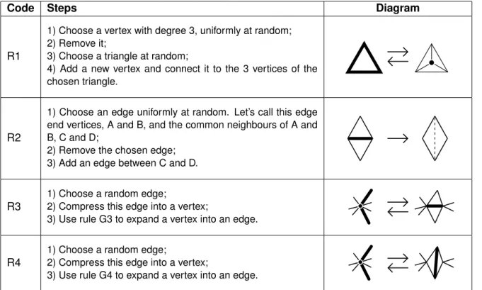
Code Steps Diagram
R1
1) Choose a vertex with degree 3, uniformly at random; 2) Remove it;
3) Choose a triangle at random;
4) Add a new vertex and connect it to the 3 vertices of the chosen triangle.
R2
1) Choose an edge uniformly at random. Let’s call this edge end vertices, A and B, and the common neighbours of A and B, C and D;
2) Remove the chosen edge; 3) Add an edge between C and D.
R3
1) Choose a random edge;
2) Compress this edge into a vertex;
3) Use rule G3 to expand a vertex into an edge.
R4
1) Choose a random edge;
2) Compress this edge into a vertex;
3) Use rule G4 to expand a vertex into an edge.
Table 3.3: Rules for relaxation description.
Chapter 4
Results
4.1
Initial results
Using the relations obtained in 2.6, we can calculate some network characteristics. To calcu-late the average degree, we can usehki = 2E/N [22]:
hki = 6N − χ
N (4.1)
Given the constraints of our surface, only in the case were the topology is the same as a torus (χ = 0), the mean degree is exactly hki = 6. In all other cases, this value is only achieved asymptotically for very large networks.
The clustering coefficient measures the probability that two neighbours of a vertex are also neigh-bours between themselves. There are two different clustering coefficients. We have the network clustering coefficient [20] given by:
C = 3 number of loops of length 3 in a network
number of connected triples of nodes (4.2)
In the case of our networks, we will have:
C = 3 P F iki(ki− 1)/2 = 12 N − χ N (hk2i − hki) = 2 hki hk2i − hki (4.3) We see that for networks with diverging second moment,C = 0.
There is another clustering coefficient, the average local clustering coefficient. To calculate it, we obtain the local clustering for each vertex, that is given by:
Cj =
tj
kj(kj− 1)/2
(4.4)
wheretj is the number of connections between the neighbours of vertexj.
In our networks, the number of connections between the neighbours of a given vertex is equal to the vertex’s degree. We can calculate the average local clustering coefficient:
C = 1 N X j Cj = X k P (k) k k(k − 1)/2 = X k P (k) 2 k − 1 (4.5)
is the case of a 2D triangular regular mesh or a torus, the average local clustering isC = 2/5
4.2
Experimental method
In order to observe the evolving characteristics of the network grown or relaxed by each rule, we made a series of computer simulations. Given the ensemble approach we are using, (section 2.2), in order to measure some quantity we would need to average it using all the ensemble of possible realizations. But that is impossible. So, for each rule, we generate a sufficient number of networks of that ensemble, so that we can obtain average results with low noise.
These networks must be large enough, approximating the ”infinite” case, because there are some quantities that can be only measured for very large networks, as is the case of dimensionality or average distance growth with system size.
One of the limitations of finite size networks is a cut-off in the degree distribution. That will limit, for example, the observation of power law behaviour for high degree values. We can have rough estimation the cut-off,kcut, using:
N Z ∞
kcut
P (k) = 1 (4.6)
For many rules, we obtained degree distributions that approached power-lawP (k) ∼ k−γ or ex-ponentialP (k) ∼ exp(−βk)distributions. We can obtainkcut ≈ k0N1/(γ−1) for a power law and
kcut ≈ k0+β1 ln Nfor exponential distribution, in whichP (k < k0) = 0.
To have a better sense of the computational constrains of this simulations, section 6.9, in the appendix, has further information.
4.3
Rules for growth
Rule G1
After a considerable number of steps (226), we obtained the following degree distribution:
10-12 10-10 10-8 10-6 10-4 10-2 100 100 101 102 103 104 105 P(k) k sim. data PMF(k)
Figure 4.1: Rule G1. Degree distribution for system sizeN = 226.
Simulation data and analytical distributionPM F(k)of equation 4.10
Figure 4.1 shows that the degree distribution follows a power law, such thatP (k) ∼ kγ, with
γ ≈ 3.
This is happening due to the preferential attachment mechanism that is operating in this sys-tem. In the BA model, we know that if the new vertex connects to old vertices proportionally to their degree, a power law distribution will emerge given enough steps.
In this rule’s case, we see that a by choosing a triangle uniformly at random, we are in fact choos-ing vertices proportionally to their degrees, because the number of triangles adjacent to a vertex is equal to its degree.
Using a mean field theory, (see section 6.5), we can derive the exact degree for the infinite case. Assuming that there are no degree correlations, then we can build the following master equation:
N (k, t + 1) = N (k, t) + 3P (k − 1, t)k − 1
hki − 3P (k, t) k
hki+ δk,3 (4.7)
in whichtis the step number. This equation shows in the left hand side the number of vertices with degreekin timet + 1that will be equal to the current number of nodes plus 3 chances of obtaining vertices from degreek −1using a probability proportional to their degree, minus loosing 3 vertices of degreek, with probability also proportional to their degree.
Fort → ∞, we can approximateN (k) ≈ tP (k), andhki ≈ 6, then we will get
P (k) = 1
2(k − 1)P (k − 1) − 1
2kP (k) + δk,3 (4.8)
Reorganizing the terms, we will obtain the recursion relation:
P (k) = (k − 1)
(k + 2)P (k − 1) + 2
(k + 2)δk,3 (4.9)
Assuming thatP (k < 3) = 0, that will lead to:
P (k) = 24
If we recall plot 4.1, we see that this analytical result fits perfectly the simulation data. Also, our assumption about non-existent correlations is supported by fig. 4.2b, were the Pearson Coeffi-cient is approximating 0 for large networks sizes.
1 2 3 4 5 6 7 8 9 10 11 100 101 102 103 104 105 106 107 108 <l> N
(a) Average distancehlievolution with system sizeN.
-0.5 -0.45 -0.4 -0.35 -0.3 -0.25 -0.2 -0.15 -0.1 -0.05 0 100 101 102 103 104 105 106 107 108 r N
(b) Pearson coefficientrevolution with system sizeN.
Figure 4.2: Rule G1. Average distance and Pearson coefficient evolution.
Looking at the distance evolution in plot 4.2a, we see that the mean distance evolution is propor-tional tolog t.
We can explain this behaviour using the following arguments:
A path passing through the new vertex has to pass through two of the vertices of the chosen tri-angle. But we can shortcut that path, using the direct connection between these two old vertices. So, a path passing through the new vertex cannot be minimal. Therefore, the shortest distances between old vertices will not change. The only variation of the mean distance can only come from the distances between the other vertices and the new vertex.
Usinghli(t)ias the mean distance to vertexiat timet, then, the mean distance at timet + 1is:
hl(t + 1)i = 1 N + 1 N +1 X i=1 hli(t + 1)i = 1 N + 1(N hl(t)i + hlN +1(t + 1)i) (4.11)
Fort → ∞, assuminghlN +1(t + 1)i ≈ hl(t)i + 1andN + const. ≈ t, then:
∂
∂thl(t)i ≈ 1
t (4.12)
So, we see that the variation of average distance is proportional to the inverse of time, giving us a logarithmic growth.
If we calculate the average local clustering coefficient, using the degree distribution 4.10 in equa-tion 4.5, we will obtainC = 23.
Given it’s characteristics of growth, this network can be considered small-world.
Rule G2
Plot 4.3a shows that the degree distribution also follows a power law,P (k) ∼ kγ, withγ ≈ 4.
10-12 10-10 10-8 10-6 10-4 10-2 100 100 101 102 103 104 P(k) k sim. data PMF(k)
(a) Rule G2. Degree distribution for system sizeN = 226.
Simulation data and analytical distributionPM F(k)of
equation 4.15. 100 101 102 100 101 102 103 104 105 106 107 108 <l> N
(b) Rule G2. Mean distancehlievolution
with system sizeN.
Figure 4.3: Rule G2. Degree distribution and average distance evolution.
This can be explained by the similar behaviour to rule G1, where vertices with higher degrees have a better chance to increase their degree. Each vertex has a perimeter of edges that connect all its neighbours. The number of edges of this perimeter is equal to the vertex degree. If an edge of this perimeter is chosen, then this vertex will increase it’s degree.
Using the method of mean field, used in the derivation of the degree distribution in rule G1, we will obtain the master equation. Again, no degree correlations are used:
N (k, t + 1) = N (k, t) + 2P (k − 1, t)k − 1
hki − 2P (k, t) k
hki+ δk,4 (4.13)
leading to the recursion:
P (k) = k − 1
k + 3P (k + 1) + 3
(k + 3)δk,4 (4.14)
Assuming that for larget,P (k < 4) = 0, then the exact degree distribution is:
P (k) = 360(k − 1)!
(k + 3)! (4.15)
that for largek, it will beP (k) ∼ k−4.
Plot 4.3b does not show a clear relation between the evolution of mean distance with system size. We have tried to grow the network as large as possible, but even then the relation with sys-tem size is not obvious. So, instead of trying to fit a function, we obtained the derivative in log-log space, giving us the exponent of a local fitting of a power law. ForN = 226, we have obtained an exponent around (hli ≈ N0.17). The procedure is better explained in appendix 6.6
The analytical derivation of the mean distance of this rule could not be deduced as easily as in rule G1. The modification that G2 introduces, by dividing an edge, will only affect shortest paths that use that same edge, if they have no shortest alternative. To calculate the new average distance, we will need a strategy to quantify the shortest paths that are affected, a task that is much harder that in rule G1.
Rule G3
This rule is the most simple application of the expansion mechanism (recall section 3.1). Looking to it’s degree distribution, we can see that it achieved one of the highest values ofγ ≈ 6 of all simulations (see table 4.1). This means that high degree nodes are very hard to create. We can explain that by the rule’s mechanism itself, that splits the neighbours of the chosen middle vertex between itself and a new vertex. Clearly this mechanism reduces the chances for the survival of high degree vertices.
The mean distance variation with system size has an exponent≈ 0.19, what is coherent with the dimensionality above5.
Rule G4
Being a variation of rule G3, we wanted to see what is the impact of introducing the flip as the end step. It seems that the dimensionality has decreased and the degree distribution has a lower
γ. Because a lowerγ usually means smaller diameters, we were expecting that it would lead to a higher dimensionality. In fact, at each step, the extra flip is increasing 2 degrees for the two neighbours of the middle vertex, explaining the lower γ. The flip is also modifying the average distance in two ways: it is increasing the distance for some shortest paths that pass in the middle vertex, but is lowering the distance for shortest paths that pass in the two edges formed by the middle vertex and it’s two neighbours.
Rule G5
We wanted to know how the choice of edges, instead of vertices (like in G3), would affect the net-work. This method of choosing elements of the surface, introduces a preferential choice because the higher the degree of a node is, the more chances has to be chosen.
The degree distribution shows a cut-off forklower than G3, showing more difficulty in generating high degree nodes. We think this is happening because the preferential choice is leading to the destruction of high degree nodes.
Looking at the result of the dimensionality, we see that it achieved a much lower dimensionality (dH ≈ 3.1), relative to G3 (dH > 5).
Rule G6
Given the minor differences between this rule and rule G5, we see that some characteristics such as the Hausdorff dimensionality are almost the same. However, the degree distribution has a cutoff at a higher degree than G5. This is because in G5, the end of the chosen edge that had a higher degree would had a higher probability to be the middle vertex. In G6, both ends had the same probability, therefore the high degree nodes in G5 had a higher chance to be destroyed than in G6.
General results of the rules for growth
Growth Network Number of P(k) hdi(N ) Spectral dim. Hausdorff
rule size (N) simulations (N = 217) dim.
G1 226 400 ∼ k−3.0(1) 0.546(4) ln N 2.2(2) ∞ G2 226 400 ∼ k−3.95(5) ∼ N0.17(2) 2.1(2) > 5 G3 226 80 ∼ k−5.9(4) ∼ N0.19(3) 1.9(1) > 5 G4 226 400 ∼ k−5.0(4) ∼ N0.27(1) 1.9(1) 3.8(1) G5 226 400 n/a ∼ N0.32(1) 1.9(1) 3.1(1) G6 226 400 ∼ exp(−0.40(1)k) ∼ N0.30(1) 1.9(1) 3.3(1)
Table 4.1: Rules for growth. Simulation results.
The results show that various degree distributions and mean distance evolutions could be achieved by simply using different rules for growth. Nevertheless, the spectral dimension for all rules is around 2, what is not so surprising given that the surfaces are 2D manifolds. The surfaces used in this measurement were very small, given the constraints of the method used to measure it, which needed to obtain the eigenvalues of a matrix with sides equal to the number of nodes.
In terms of structural evolution, we used the Pearson coefficient (see section 6.4) which for every rule showed an evolution that converges to a stable value for large networks.
0 0.05 0.1 0.15 0.2 0.25 0.3 0.35 0.4 100 101 102 103 104 105 106 107 108 exponent N G1 G2 G3 G4 G5 G6 log
(a) Exponent of power-law local fitting evolution with time.
-0.5 -0.45 -0.4 -0.35 -0.3 -0.25 -0.2 -0.15 -0.1 -0.05 0 100 101 102 103 104 105 106 107 108 109 r N G1 G2 G3 G4 G5 G6
(b) Pearson coefficient evolution with time Figure 4.4: Rules for growing. Exponent of average distance and Pearson coefficient evolution for various rules.
Plot 4.4a shows the evolution of the measurement of the power-law exponent with system size (see details of this method in 6.6). For large system size, every network show an assimptotically evolution to a constant value. We see that rule G1 exponent goes to 0, that is almost the same behaviour that a log has.
The Pearson coefficient (4.4b) shows an initial strong anticorrelation from the initial surface. After enough steps we see this coefficient growing thowards 0 (G1 and G2) or stabilizing in a constast value (G3 and G4).
4.4
Variations of rule G3
G3.1This rule was designed to observe the impact of selecting the 2nd neighbour, during the expan-sion procedure. 0 0.5 1 1.5 2 2.5 3 3.5 4 100 101 102 103 104 dH r 218 220 222 224 226 228 230
Figure 4.5: Rule G3.1. Hausdorff dimensiondHevolution with radiusr
for various system sizesN.
The dimension of the network clearly diminished fromdH ≈ 5(G3) todH ≈ 3.7. So we see that this biased division mechanism has influenced the dimensionality, as expected.
Also, the high exponentγ ≈ 6.3of the degree distribution, clearly demonstrates the destruction of high degree nodes. In rule G3, given a less biased neighbour selection, the exponent was lower,
γ ≈ 5.9.
G3.2
This rule forced the choice of 2nd neighbour to be next to the 1st neighbour, given the order of neighbours around the middle vertex.
0 2 4 6 8 10 12 100 101 102 dH r 218 220 222 224 226 228 230
Figure 4.6: Rule G3.2. Hausdorff dimensiondHevolution with radiusr
for various system sizesN.
This rule is very similar to G1. We already know that the mean distance of G1 evolves with the logarithm of system size, so we expected that the same happened with this rule, what was confirmed by the experimental results. The growing dimension with system size indicates a pos-sible infinite dimensionality.
G3.3
The choice mechanism in this rule is clearly a preferential choice of high degree vertices. There-fore, high degree nodes are being destroyed, leading to a more uniform degree distribution and a lower dimensionality than G3.1.
G3.4
This rule clearly chooses an vertex with preference proportional to its degree. The impact of this choice is almost the same as in G3.3 and the dimensionality and distance evolution reflects this similarity.
G3.5
The difference to rule G3.4 is that we forced the choice of the 2nd neighbour to be the opposite edge to the first chosen edge. This had almost no impact in dimensionality. Maybe the preferen-tial choice by vertex degree is enough to achieve this dimensionality.
G3.6
In this last variation, we forced the choice of the middle vertex to be the edge’s highest degree end. This had some impact in dimensionality, achieving dH ≈ 2.7, the lowest one of all experi-mented rules.
Growth Network Number of P(k) hdi(N ) Spectral dim. Hausdorff
rule size (N) simulations (N = 217) dim.
G3.1 226 80 ∼ k−6.3(3) ∼ N0.27(1) 1.9(2) 3.7(2) G3.2 226 80 ∼ k−4.4(4) 0.78(4) ln N 2.2(2) ∞ G3.3 226 80 ∼ exp(−1.0(1)k) ∼ N0.36(1) 1.9(2) 2.8(1) G3.4 226 80 ∼ exp(−0.7(1)k) ∼ N0.34(1) 1.9(3) 2.9(1) G3.5 226 80 ∼ exp(−0.5(1)k) ∼ N0.34(1) 1.9(2) 2.9(1) G3.6 226 80 ∼ exp(−1.4(1)k) ∼ N0.38(1) 1.9(2) 2.65(5)
Table 4.2: Variations of rule G3. Simulation results.
0 1 2 3 4 5 6 7 8 9 10 100 101 102 103 104 dH r G3 G3.1 G3.2 G3.3 G3.4 G3.5 G3.6
(a) General plot.
0 0.5 1 1.5 2 2.5 3 3.5 4 100 101 102 103 104 dH r G3 G3.1 G3.2 G3.3 G3.4 G3.5 G3.6 (b) Detail plot. Figure 4.7: Variations of G3. Hausdorff dimension variation with radius
for various rules. System sizeN = 228.
0 2 4 6 8 10 12 105 106 107 108 109 1010 dH max. N G3 G3.1 G3.2 G3.3 G3.4 G3.5 G3.6
(a) General plot.
2 2.5 3 3.5 4 105 106 107 108 109 1010 dH max. N G3 G3.1 G3.2 G3.3 G3.4 G3.5 G3.6 (b) Detail plot.
Figure 4.8: Variations of G3. Maximum Hausdorff dimension variation with system size, for various rules.
What can we conclude from all these variations? It seems that destroying high degree nodes is a good method to achieve low dimensionalities. Nevertheless, the uniformity of degree, such in a regular surface (eg: icosphere), was far from being reached. Likewise, Hausdorff dimension 2 was also very difficult to achieve, being 2.7 the closest we obtained.
A interesting feature of all these variations of G3 (except for G3.2) was the uniformity of the spec-tral dimension, with almost all of the rules going arounddS≈ 1.9.
4.5
Rules for relaxation
There are two main stages when making these simulations. The first stage is the evolution from an initial surface until the equilibrium stage, and the equilibrium stage itself.
Because we are using the rules for relaxation, the number of elements of a network is fixed, there-fore, in order to obtain quantities that vary with system size, we had to run the rule for different system sizes until they reach the equilibrium stage.
Although ideally we would want to relax very large networks, the number of steps needed to reach the equilibrium stage also grow with system size, taking too long to simulate system sizes above
N > 105.
Another problem is related to initial conditions, what should be the initial surface to relax? What we have observed observerd is that the inital surface does not matter. So, all rules begun with the icosphere (see section 6.8), except rule R1.
Rule R1
This rule begins by relaxing a surface grown by rule G1. Comparing the results (table 4.3), we see there is a clear evolution from rule G1. This shuffling of vertices, has proven to be a effective way of changing the structure of the network.
Rule R2
The inital surface, the icosphere, aproximated delta degree distribution around 6. After relaxation, the network achieved a exponential distribution, revealing a structural change. In figure 4.9a, we see this evolution from initial(red) to final(blue) distribution.
10-7 10-6 10-5 10-4 10-3 10-2 10-1 100 100 101 102 P(k) k
(a) Rule G2. Degree distributionP (k)evolution with time.
Initial time in red, final time in blue.
20 30 40 50 60 70 80 90 100 101 102 103 104 105 106 107 108 109 1010 <l> t
(b) Rule G2. Mean distancehlievolution with time.
Figure 4.9: Rule G2. Network characteristics evolution with time.
We see that the average distance evolution with time is not monotonic. There is a point where the average distance goes to a minimum, and then rises until it reaches equilibrium. This mini-mum is persistently present for various initial sizes.
If the starting surface was a small world surface, the evolution was somewhat different, but we see an inflexion about the same time.
The time of minimum also evolves, but at a different rate of the initial time for the equilibrium. We can compare two speeds of growth with the size of system: initial time of equilibrium stage
and time of minimum distance. 102 103 104 105 106 107 108 109 1010 102 103 104 105 106 t N tmin teq N1.55 N1.7
Figure 4.10: Rule R2. Evolution of time of minimum distancetminand time of start of equilibriumteq
with system sizeN. An icosphere is used as the initial surface.
Rule R3
This rule combines rules G3 with it’s inverse process. Comparing with the simple growth of G3, we see that the degree distribution has a lower γ. This is related to the compressing process which creates high degree nodes.
Rule R4
Rule R4 is quite similar to rule R3, except an extra flip in the expansion phase. The resulting de-gree distributions, distance evolutions and dimensionalities are quite similar. The extra flip gave R4 a higherγ and a lower dimensionality.
General results of the rules for relaxation
Growth Network Number of P(k) hdi(N ) Spectral dim. Hausdorff
rule size (N) simulations (N = 215) dim.
R1 215 32 n/a ∼ N0.47(6) 1.3(1) 2.1(2)
R2 217 20 ∼ exp(−0.31(1)k) ∼ N0.30(2) 1.5(2) > 3
R3 217 20 ∼ k−3.0(2) ∼ N0.20(2) 1.3(2) > 4
R4 217 20 ∼ k−3.3(1) ∼ N0.25(3) 1.5(2) > 3.5
Table 4.3: Rules for relaxation. Simulation results.
0 20 40 60 80 100 120 140 160 180 100 101 102 103 104 105 106 107 108 109 1010 <l> t R1 R2 R3 R4
(a) Average distancehlievolution
with steps of relaxationt
-0.25 -0.2 -0.15 -0.1 -0.05 0 0.05 100 101 102 103 104 105 106 107 108 109 1010 r t R1 R2 R3 R4
(b) Pearson coefficientrevolution
with steps of relaxationt
Figure 4.11: Rules for relaxation. Average distance and Pearson coefficient evolution with time for various rules.
The dimension of the relaxed networks is quite small, because the number of steps needed to reach the equilibrium phase increases above linearly with system size. This growth can be ob-served in plot 4.10.
Plots 4.11a and 4.11b show evolving characteristics during the relaxation process, which demon-strate the transition between a starting structure to another kind of structure. We see that rule R1 has a different evolution relative to the other ones, given that its initial structure is a network built by R1, instead of the icosahedron for the all the others.
After a large number of steps, both characteristics stabilize in constant values, which is a sign of an equilibrium phase.
Rules R2, R3 and R4, show an evolution of average distance which is non-mononotic, achieving an average distance lower that the average distance at the equilibrium phase.
One of the most surprising characteristics of these algorithms is the spectral dimension. Given the relaxing purpose of these rules, it was expected that these rules would ”uniformize” the struc-ture, leading to a spectral dimension that would reflect the dimension of the embedding space. But what we have found is that all of these relaxing algorithms obtained a dimensiondS ≈ 1.5 and even lower. Due to computational limitation, the largest network in which we measured this dimension had sizeN = 215. So the measureddS still might change significantly, and may even approach2, for larger networks.
4.6
n
-dimensional results
In order to derive the degree evolution of then-dimensional versions of rules G1 and G2, we will assume that there are no correlations. Assuming that we can compare the edge introduction to a preferential attachment operation, we can compare this to the model presented in [20, 23]. In that model, the exponentγ inP (k) ∼ kγis given byγ ≈ 3 + Am in whichAis the initial attrac-tiveness of a site, given byPchoice(k) ∼ k + A, andm, which is the number of links introduced in the model at each step.
Let’s call Sn the number ofn-simplexes incident to a vertex. The starting object of a manifold composed ofn-simplexes, will be ann + 1-simplex, therefore each vertex of this initial manifold
has degreek = n + 1andSn= n + 1.
Rule 1 (n-dimensional)
Let’s suppose that incident to a vertex, we have a new vertex. That will insertn n-simplexes and remove 1n-simplex. The variation of simplexes is then∆Sn= n − 1.
Each new vertex has degreen + 1, therefore we can write:
Sn(k) = n + 1 + (k − (n + 1))(n − 1) (4.16) The probability of choice is then Pchoice(k) ∼ k − (n + 1) + n+1n−1, obtaining a function A =
n+1
n−1 − (n + 1). The number of new edges is equal to the number of vertices in an-simplex, thereforem = n + 1, leading to:
γ = 2 + 1
n − 1 (4.17)
Rule 2 (n-dimensional)
In this case, we have two different mechanisms of attraction. One of them is related to then − 1 -simplex that is divided and another is for the two vertexes of the two n-simplexes that share a
n − 1simplex.
The number ofn − 1simplexes for each vertex,Sn−1is dependent on the number ofn-simplexes incident to the vertex. Given that eachn-simplex hasn + 1faces (n − 1-simplexes), and that each of it’s vertexes is onnof those, then the number of faces incident to each vertex is:
Sn−1= Sn
n
2 (4.18)
in which the 1/2 factor comes from the repetition of faces, which are shared by pairs of n -simplexes. The probability of choice for each vertex is thenPchoice∼ Sn, fornnew edges. In the other hand, the for each n-simplex incident to a vertex, there is one face that does not include that vertex, so the number of faces is equal to the number ofn-simplexes. Therefore the probability of choice isPchoice∼ Snfor 2 new edges.
We see that both choices of vertex are proportional to the number of n-simplexes incident to it. If we recall Rule 1 (n-dimensional), we will haveA =n+1n−1− (n + 1). The number of new edges will ben + 2. Therefore the exponent will be:
γ = 2 + 2n
(n − 1)(n + 2) (4.19)
Recalling the results forn = 2(rule G2), we know thatγ = 4, but equation 4.19 givesγ = 3. In fact, the model we are using to obtain the exponent, assumes that each new vertex has a degree equal to the number of new connections introduced in the model, but for n = 2 that is false. This can be solved by considering that every new vertex has an initial attractivenessA = 2, so
γ = 3 + 22 = 4as it should be.