SRef-ID: 1432-0576/ag/2005-23-1317 © European Geosciences Union 2005
Annales
Geophysicae
Magnetosheath waves under very low solar wind dynamic pressure:
Wind/Geotail observations
C. J. Farrugia1, F. T. Gratton2, G. Gnavi2, H. Matsui1, R. B. Torbert1, D. H. Fairfield3, K. W. Ogilvie3, R. P. Lepping3, T. Terasawa4, and T. Mukai, Y. Saito5
1Space Science Center and Department of Physics, University of New Hampshire, NH, USA
2Instituto de F´isica del Plasma, CONICET and FCEyN, University of Buenos Aires, Buenos Aires, Argentina 3NASA Goddard Space Flight Center, Greenbelt, MD, USA
4Department of Earth and Planetary Physics, University of Tokyo, Tokyo, Japan 5Institute of Space and Astronautical Sciences, Kanagawa, Japan
Received: 2 October 2004 – Revised: 11 February 2005 – Accepted: 24 February 2005 – Published: 3 June 2005
Abstract.The expanded bow shock on and around “the day the solar wind almost disappeared” (11 May 1999) allowed the Geotail spacecraft to make a practically uninterrupted 54-h-long magnetosheath pass near dusk (16:30–21:11 magnetic local time) at a radial distance of 24 to 30RE (Earth radii). During most of this period, interplanetary parameters varied gradually and in such a way as to give rise to two extreme magnetosheath structures, one dominated by magnetohydro-dynamic (MHD) effects and the other by gas magnetohydro-dynamic ef-fects. We focus attention on unusual features of electromag-netic ion wave activity in the former magnetosheath state, and compare these features with those in the latter. Mag-netic fluctuations in the gas dynamic magnetosheath were dominated by compressional mirror mode waves, and left-and right-hleft-and polarized electromagnetic ion cyclotron (EIC) waves transverse to the background field. In contrast, the MHD magnetosheath, lasting for over one day, was devoid of mirror oscillations and permeated instead by EIC waves of weak intensity. The weak wave intensity is related to the prevailing low solar wind dynamic pressures. Left-hand larized EIC waves were replaced by bursts of right-hand po-larized waves, which remained for many hours the only ion wave activity present. This activity occurred when the mag-netosheath proton temperature anisotropy (=Tp,⊥/Tp,k−1) became negative. This was because the weakened bow shock exposed the magnetosheath directly to the (negative) temper-ature anisotropy of the solar wind. Unlike the normal case studied in the literature, these right-hand waves were not by-products of left-hand polarized waves but derived their energy source directly from the magnetosheath temperature anisotropy. Brief entries into the low latitude boundary layer (LLBL) and duskside magnetosphere occurred under such inflated conditions that the magnetospheric magnetic pres-sure was insufficient to maintain prespres-sure balance. In these
Correspondence to:C. J. Farrugia ([email protected])
crossings, the inner edge of the LLBL was flowing sun-ward. The study extends our knowledge of magnetosheath ion wave properties to the very low solar wind dynamic pres-sure regime.
Keywords. Ionosphere (Wave-particle interactions) – Mag-netospheric physics (Magnetosheath) – Radio science (Waves in plasma)
1 Introduction
There are two major approaches to modeling the flow of the shocked solar wind around the terrestrial magnetosphere. In the traditional approach, known as the convected gasdynamic model (CGDM) and associated with the names of Spreiter and coworkers (Spreiter et al., 1966; Spreiter and Alksne, 1969; Spreiter and Stahara, 1980), the solution for the flow around a blunt body is obtained first, neglecting the magnetic forces in the momentum equation. After that, the magnetic field is derived by passive convection in the gas dynamic flow field, using the frozen-in field condition. Although this kine-matic approach decouples the solution of the flow from that of the field, it has been widely successful in explaining the gross features of the magnetosheath of magnetized planets. It becomes increasingly reliable as the Alfven Mach num-ber of the solar wind (MA) increases because in the momen-tum equation thej×Bforce scales as MA−2 (Spreiter et al., 1966). QuantityMA (MA2≡Vp2/VA2=ρV
2
p/(B2/µ0), where
Fig. 1. The orbits of three near-Earth spacecraft data from which are discussed in this study. The top and bottom panels show, re-spectively, GSE XY and XZ projections. The interval plotted is 14:00 UT (10), 01:00 UT (13),∼3 h longer than Geotail’s magne-tosheath passage near dusk, which started at 16:40 UT (10). The different colors correspond to different days.
a region of strong field and low density forms adjacent to the sunward side of the magnetopause, called the plasma de-pletion layer (PDL). Its thickness is proportional to 1/MA2
(Farrugia et al., 1995)
In the second approach, the influence of the interplanetary magnetic field (IMF) on the magnetosheath flow is included from the start (see, for instance, Midgley and Davis, 1963; Lees, 1964; Zwan and Wolf, 1976; Erkaev, 1988; Wang et al., 2003). In this treatment the PDL arises naturally and defines a MHD–dominated region whose flow and wave properties are different from those in the rest of the magnetosheath. On the dayside the flow is of the stagnation line type (Sonnerup, 1974; Phan et al., 1994). As a result, at the magnetopause the flow tends to align itself perpendicular to the local mag-netic field. As the magnetopause is approached, the tempera-ture anisotropy of the protons,Ap≡Tp,⊥/Tp,k−1 (where the symbols “⊥” and “k” are defined with respect to the back-ground magnetic field direction) increases. Further, Ap is found to anticorrelate withβp,k, as predicted by theory (Gary and Lee, 1994; Gary et al., 1994) and confirmed experimen-tally ( Anderson and Fuselier, 1993; Anderson et al., 1991, 1994).
Whereas the main body of the magnetosheath is high beta and the condition to de-stabilize the mirror mode is generally marginally satisfied (Phan et al., 1994; Hill et al., 1995), in the lowβ−high, positiveApPDL the mirror mode is stable, and instead left-hand polarized electromagnetic ion cyclotron waves (EICWs) transverse to the field are excited, as first reported by Fairfield (1976). Right-hand polarized EICW power is lower than the left-hand power and is thought to be generated as a secondary emission (“daughter” waves) from the left-hand waves. The PDL may thus be characterized by a special type of wave activity, the EIC waves. One main objective of this paper is to show that under very lowPdyn this PDL-type wave activity extends to the main body of the magnetosheath (as judged by the distance of the spacecraft from a model magnetopause surface). Another is to show that the right-hand polarized EICWs are directly generated by the negative temperature anisotropy (and not as secondary waves) at a time when the bow shock is weak.
In an experimental work, we shall analyze ion wave activ-ity in the magnetosheath under lowPdynconditions (at nearly constantB), which occurred over the extended period 10–11 May 1999. This is a much studied event, and 11 May 1999, has been dubbed “the day the solar wind almost disappeared” because solar wind densities decreased to low values of or-der 0.2 cm−3andPdynto∼0.10 nPa, see special editions of Geophys. Res. Lett. (2000) and J. Geophys. Res. (2000). In particular, the bow shock was displaced to its most sunward position on record, about 50RE upstream of Earth (Fairfield et al., 2001). Because of the dilated magnetosphere and bow shock, the spacecraft Geotail spent an uninterrupted stretch of 54 h in the magnetosheath. There it observed many effects due to the strong influence of the IMF on the magnetosheath, which may be isolated and studied by comparing them with a long segment of the same pass when MHD effects were much attentuated. An important feature is that interplanetary parameters change very slowly during the long-duration den-sity decrease, so that the magnetosheath traverses essentially a sequence of quasi-steady states.
The layout of the paper is as follows. After a discussion of interplanetary conditions recorded by Wind and IMP 8, we discuss in turn the magnetic field, plasma, and wave obser-vations made by Geotail in the magnetosheath. Wave theory results are discussed in conjunction with the observed elec-tromagnetic ion wave spectra. We then discuss the relevance of these findings to our knowledge of the magnetosheath.
2 Wind and IMP 8 observations
2.1 Spacecraft orbits
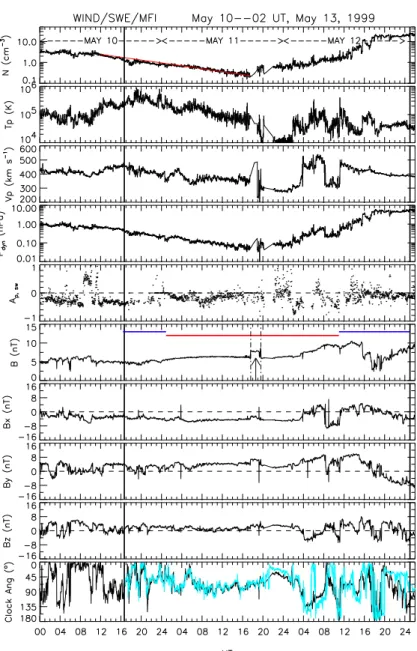
Fig. 2.Plasma and magnetic field data from the SWE and MFI investigations on Wind. GSM coordinates are used. The time resolution of the data sets are∼90 s (plasma) and 3 s (magnetic field). The vertical lines bracket the interval when Geotail was in the magnetosheath. The arrow in the 5th panel marks the time when the bow shock passed over Wind. For details about the panels, see text. The light blue trace in the bottom panel is an overlay of the clock angle measured by Geotail in the magnetosheath when no lag is assumed between Wind and Geotail measurements.
the spacecraft was executing a swing-by manoeuvre near the moon (symbol “M”) on 12 May.
Geotail orbits at a radial distance which varies between 24.2 to 30.3RE (Earth radii), and covers a magnetic local time (MLT) range from 16:25 to 21:10 MLT, with the space-craft staying close to the ecliptic plane. Wind was on the opposite side of the Sun-Earth line to Geotail and travel-ing sunward. The inter-spacecraft separation orthogonal to the Sun−Earth line lies in the range 46 to 64RE. IMP 8 is more favorably located, but no plasma data are available from this spacecraft. After introducing the Wind observations in Figs. 2 and 3, we shall cross-correlate Wind and IMP 8 mea-surements to ascertain that Wind data are appropriate for this
study, since a distance of∼60REperpendicular to the Sun-Earth line is comparable to typical correlationlengths of the IMF in this direction (Richardson and Paulerena, 2001; Mat-sui et al., 2002).
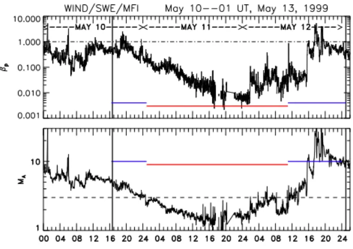
Fig. 3. The proton plasma beta and the Alfven Mach number de-rived from Wind measurements. The vertical guidelines bracket the duration of Geotail’s magnetosheath interval. Two regimes in
βp−MA space are indicated by the two colored horizontal bars:
MHD-dominated in red; gas dynamic-dominated in blue.
10 May, 02:00 UT, 13 May 1999. The temporal resolutions of the data are 90 s for the plasma and 3 s for the magnetic field. TheAp,swdata are 3-min averages. The vertical lines delimit the time interval when Geotail was inside the magne-tosheath. (The colored horizontal bars in theBpanel and the light blue trace in the clock angle panel are explained below.) Aside from a brief interval∼17:40–19:40 UT (11), indicated by an arrow in panel 6, when the sunward-expanding bow shock crossed Wind, this spacecraft was positioned upstream of the bow shock, being at (32.0,−29.8, 17.8)REand (47.7,
−35.3, −5.1)RE (GSE coordinates) at 16:00 UT, 10 May and 01:00 UT, 13 May, respectively. (For convenience, we shall use below the notation x UT (y) to denote x UT on May y, 1999.)
At Wind, the density started its steady decrease from val-ues of∼3 cm−3at 11:00 UT (10), reaching lowest values of
∼0.2 cm−3when the bow shock passed over the spacecraft at∼18:00 UT (11). The progressively more tenuous wind is also progressively colder and slower. In contrast, the total field is relatively steady (<B>=5.60±0.68 nT) and is char-acterized by a negativeBx, a positiveBy and has a slightly northward orientation on average. Quantity Pdyn reaches lowest values of ∼0.07 nPa. The temperature anisotropy,
Ap,swis generally negative with intermittent positive values. The solar wind density decreases asnsw=2.45 e−0.08T (T in hours), shown by the red line in the first panel of Fig. 2. This almost linear descent amounts to a steady decrease of ∼0.1 cm−3h−1 in np (and 0.02 nPa h−1 inPdyn), slow enough for conditions in the magnetosheath to be considered as changing in a quasi-steady fashion.
For the same interval as Fig. 2, Fig. 3 shows the plasma beta βp and the Alfven Mach number MA derived from the Wind measurements. During the density decrease, the plasma beta drops by about two orders of magnitude, from
values of∼1 to∼0.01, returning to typical solar wind values of∼1 in the last 10 h of the interval. ParameterMA, which starts from∼7, reaches lowest values of ∼1.3, only to re-turn to values≥10 in the last 10 h. Thus there is a∼1.5-day period, marked by the horizontal red bar, when parameters
Pdyn<0.3 nPa, MA<3 (dashed line), andβp<0.1. These are different from typical solar wind conditions at 1 AU, i.e.
MA≥10,βp≥1, andPdyn=2.2 nPa.
When the density starts to recover after∼00:00 UT (12), the interplanetary field and flow parameters are highly vari-able, and their magnitudes and amplitudes of variation are much larger (Fig. 2). The density and dynamic pressure approach steady values of∼20 cm−3and∼5.5 nPa, respec-tively. These last 10 h contrast sharply with the preceding interval and are characterized byMA≥10 andβp≥1, as is typical of the solar wind at 1 AU under, however, compressed conditions.
To summarize: Two types of solar wind are influencing the magnetosheath structure during the period of study: An extended segment where one would expect MHD effects to predominate, and another 2 segments (particularly the last 10 h) where they should be much attenuated. Does the mag-netosheath structure reflect this subdivision? Are there ef-fects which may be attributed to the lowPdyn and/orMA? These are the questions we seek to answer.
We now correlate Wind and IMP 8 magnetic field data. IMP 8 was in the solar wind for long stretches of time, and it is located on the same side of the Sun-Earth line as Geo-tail (See Fig. 1). The highest cross-correlation coefficients for 10–12 May 1999, are 0.75(Bx), 0.77 (By) and 0.76 (Bz) reached at a time lag of−3 min, i.e. IMP 8 observed the same IMF features 3 min earlier than Wind. We may thus use Wind data. Below we shall assume a propagation time between Wind and Geotail of 0 min. That this is a reasonable value may be seen from the light blue trace in the last panel of Fig. 2, which represents Geotail measurements of the clock angle, a quantity which correlates well across the bow shock (Song et al., 1992). With no lag assumed, it is seen that the agreement with Wind is very good up to∼04:00 UT (12). A shift of∼45 min appears on late 12 May since Wind and Geotail move in opposite directions. The large deviation at 06:00 UT (12) has other causes, as discussed in Sect. 3.2.1.
We next inquire why the measurements at Wind and Geo-tail may be considered as practically simultaneous for the earlier part of the interval under consideration. A minimum variance analysis of Wind magnetic field data (Sonnerup and Cahill, 1967) for the interval 10:00 UT (10)–04:00 UT (12) picks out a well defined normal. The ratio of intermediate-to-minimum eigenvalues=4.5, and the field normal to the plane,
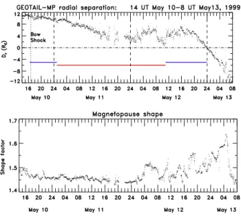
Fig. 4. For the period 14:00 UT (10) to 08:00 UT (13), the top panel shows the quantityDr, defined as the radial distance of
Geo-tail from the center of the Earth minus radial distance of the mag-netopause. The time of the bow shock crossing is indicated by the vertical guideline on the left. The bottom panel plots the shape fac-tor as a function of time, where the shape facfac-tor is defined as the terminator distance divided by the stand-off distance of the magne-topause. The model magnetosphere is that of Shue et al. (1998)
3 Geotail observations
3.1 Position with respect to the magnetopause
In order to interpret Geotail observations we first deter-mine the spacecraft’s location with respect to the magne-topause. We do this using the magnetopause model of Shue et al. (1998), where the magnetosphere shape is obtained as a function of bothPdynand IMFBz.
The top panel of Fig. 4 shows the quantityDr defined as the distance of Geotail from the model magnetopause along the radial line. The Fig. extends from 14:00 UT (10) to 08:00 UT (13). When the solar wind density is decreasing,
Dr decreases monotonically on average, mainly as a result of the expansion of the magnetosphere. The spacecraft is severalRE away from the model magnetopause, in the main body of the magnetosheath. As the pressure starts to recover, quantity Dr increases. The close approach to the magne-topause during 08:00 UT (12)−11:00 UT (12) is a result of the drop in solar wind Pdyn in this interval (Fig. 2). It is followed by a renewed magnetospheric compression. Af-ter 16:00 UT (12) when the pressure is high (∼5.5 nPa) and fairly constant,Dr decreases steadily, mainly as a result of the inward motion of the spacecraft (Fig. 1). According to the model, there should be a definitive magnetopause crossing at
∼00:00 UT (13). This value would be expected to be too early by 30–45 min because the zero-lag assumption breaks down on late 12 May and early 13 May as noted above.
The bottom panel of Fig. 4 gives an indication of the changing shape of the magnetopause. The “shape factor” plotted along the vertical axis is the ratio of the distance to the terminator to the subsolar stand-off distance in the equa-torial plane, using the Shue et al. (1998) model. Through-out the density decrease, this quantity diminishes slowly, ap-proaching a value of∼1.44 whenMA∼1. Thus according to the model the magnetosphere expands approximately self-similarly and reaches the quoted shape ratio when the bow shock is very weak/absent. The other extreme of vanishing IMF, i.e. gas dynamics, valid forMA−>∞(Spreiter et al., 1966), gives for the shape factor a value of 1.32 (Mead and Beard, 1964; see also Kivelson and Russell, 1995).
After∼02:00 UT (12), as the density recovers in the sec-ond solar wind regime, and in particular the north-south com-ponent of the IMF undergoes large changes, the magneto-spheric shape changes on short time scales and is in general blunter than before. Its most flared shape, at 05:00 UT (13) coincides with a dynamic pressure of∼10 nPa, and a large, negativeBzexcursion (not shown).
3.2 Geotail magnetosheath observations 3.2.1 Magnetic field and plasma
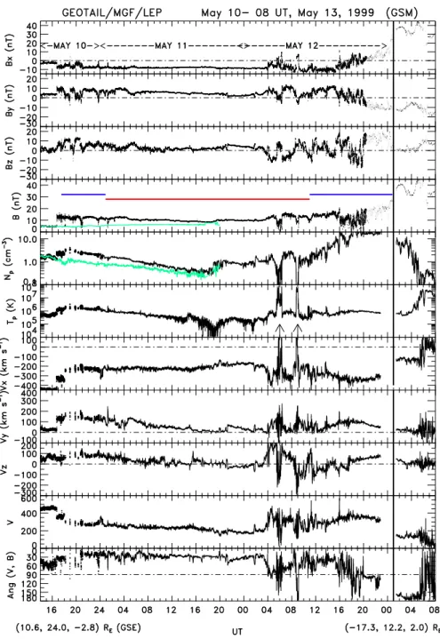
Geotail magnetic field measurements from the MGF instru-ment at 3 s resolution (Kokubun et al., 1994) and plasma data from the LEP instrument at 64 s time resolution (Mukai et al., 1994) are shown in Fig. 5 for the period 14:00 UT (10) – 08:00 UT (13). From top to bottom the panels display the GSM components of the magnetic field, the total field, the proton density and temperature, the GSM components of the velocity vector, the total bulk flow speed, and the angle be-tween the field and the velocity vectors. The green traces in theBandnppanels reproduce, with zero time lag, the corre-sponding interplanetary measurements during the solar wind density decrease for comparison. The reader is also referred to Terasawa et al. (2000) for an overview of Geotail obser-vations, and to Kasaba et al., (2000) for an overview of the Geotail electron observations.
A quasi-perpendicular bow shock (θB,n=84.5◦, the
Fig. 5.Geotail field and plasma measurements for 14:00 UT (10)–08:00 UT (13) from the MGF and LEP instruments, respectively. From top to bottom the panels display the GSM components of the magnetic field, the total field, the proton density, temperature, the GSM components of the velocity vector, the total bulk flow speed, and the angle between the field and the velocity vectors. Overlaid as green traces areBand
nppanels from Wind.
and the deflection of the velocity at the start of the second phase. Similar changes occur in the solar wind and Geotail is thus observing a convected feature; (iv) impulsive changes in most parameters at what we shall show to be brief entries into the low latitude boundary layer (LLBL)/magnetosphere at around 06:00 UT (12) and 09:00 UT (12) (arrowed). Here the field is weak and the plasma is flowing sunward. (v) the bursts of compressive field oscillations, particularly evident during Geotail’s final approach towards the magnetopause in the last 10 h (panels 1–4); (vi) the tailward stretched field
encountered on entry into the magnetosphere (panel 1) as a precursor to a substorm onset which occurred at∼04:00 UT (13) (Farrugia et al., 2000a); (vii) the definitive entry of the spacecraft into the LLBL at∼01:00 UT (13), i.e. about 1 h after the entry predicted by the model assuming zero lag, and into the magnetosphere at∼05:30 UT (13).
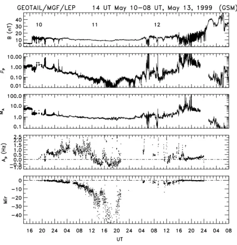
Fig. 6.For the same interval as Fig. 5, the panels show measurements by Geotail of the total field for reference, the proton beta, the Alfven Mach number, and the 1-min averages of the proton temperature anisotropy (Ap=Tp,⊥/Tp,k−1). The last panel plots the quantityMir, defined in the text.
T⊥andTkare calculated from the ion moments by referring to the magnetic field direction. There is a gap in Ap val-ues from ∼20:00 UT (11) to∼04:00 UT (12) because the magnetic field was directed in such a way that the parallel and perpendicular temperatures could not be reliably deter-mined. The last panel plots the quantityMir, defined by
Mir≡Ap−1/βp,⊥. ConditionMir≥0 is necessary one for a mirror unstable configuration. The following points may be made:
1. The main body of the magnetosheath on 00:00 UT (11)– 16:00 UT (12), when Geotail is severalRE from the magnetopause (red line in Fig. 4), is mirror stable; this is the opposite of the normal case.
2. Two large depressions in the field accompanied by a highβpand lowMAmark the two brief entries into the LLBL/magnetosphere mentioned above.
3. The plasma beta is<1 in the MHD-dominated region. Thus the main body of the magnetosheath is PDL-like by definition (Sect. 1) (Farrugia et al., 1995).
4. Initially, the temperature anisotropy is positive with val-ues≤2.5. As the pressure decreases further and the bow
shock weakens, from ∼ 11:00 UT (11) onwards, Ap decreases from values of 0.5 and becomes negative for some hours on either side of 16:00 UT (11), coinciding with the weakest bow shock.
This negative sign ofAp is the same as in the solar wind at this time (see panel 5 in Fig. 2). Values of quantityMir in the last portion of the pass, as the spacecraft approaches the magnetopause (whereβp is generally≫1 and compressive magnetic fluctuations are observed) are approximately zero. Thus in the early and later part of the pass, the mirror mode is unstable, remaining close to the marginal limit.
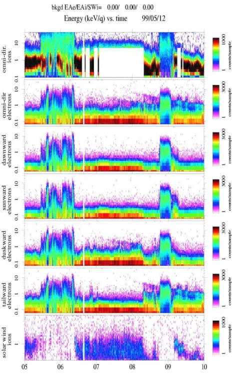
dawn-Fig. 7. Geotail measurements during 05:00 UT (12)–10:00 UT (12), in the same format as Fig. 5 except that the last panel gives the field (black trace) and proton plasma pressures.
ward, sunward, duskward and tailward, respectively, and ion fluxes of solar wind origin. Judging from the behavior of the proton density, temperature, and magnetic field strength and the spectral characteristics, the first entries are proba-bly mostly into the LLBL because some low energy electron fluxes coexist with higher energy fluxes. At the inner edge of the LLBL, the flow is sunward (Figs. 7, 8), as predicted by Sonnerup (1980), see also Sonnerup and Siebert (2003). The second crossing is into the magnetosphere proper (ab-sence of low energy electrons). Interesting in the first set of crossings is the way the magnetopause is kept in pressure balance. At these radial distances (∼30RE), the magnetic field strength and magnetic pressure are very low compared to those in the magnetosheath (fourth and last panels of the Fig. 7), but the temperature is about 2 orders of magnitude
higher, corresponding to the plasma sheet. Thus unlike the normal situation, at this inflated magnetosphere it is mainly the internal gas pressure which keeps the external pressure in check.
Compressional waves are only present for two short time segments of the pass when the proton plasma beta is large (Figs. 6, 7). Their average period is 16 s, corresponding to a frequency,f, of 0.06 Hz. According to theory, these waves are produced at zero frequency (Treumann and Baumjohann, 1997). If they are generated locally, the observed frequency
Fig. 8. From top to bottom, this figure shows Geotail measurements of the omni-directional ion and electron fluxes, the electron fluxes travelling dawnward, sunward, duskward and tailward, respectively, and ion fluxes of solar wind origin.
In the rest of the period under study, the total field is fairly steady, so that any waves have to be transverse to its direc-tion. We study these waves next.
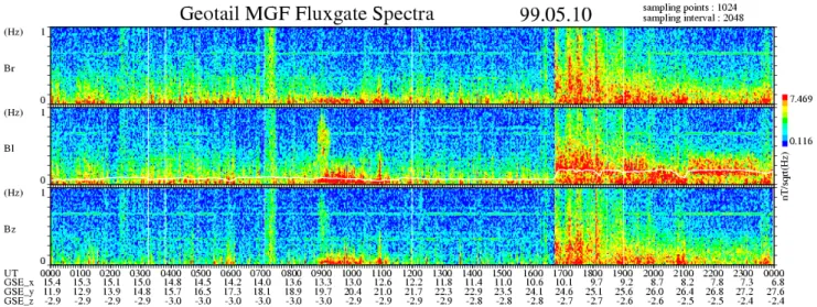
3.2.2 Electromagnetic ion waves in the magnetosheath Figures 9, 10 and 11 show frequency-time spectrograms of the magnetic fluctuations for 10, 11 May and 12−02:00 UT (13), respectively. From top to bottom the panels display the spectral amplitude of right-hand (Br), left-hand (Bl) and compressional (Bz) components, color-coded according to
the scale on the right. One Fourier transform is performed over 1024 data points. Each Fourier transform is shifted by 1024 points with respect to the previous one. The white trace in the middle panel gives the proton gyrofrequency in Hz pre-sented as 5-point smoothed averages not to obstruct the wave data during intervals of strong fluctuations inB.
Fig. 9.Frequency-time spectrograms of the magnetic fluctuations obtained from Geotail measurements for 10 May. The panels show from top to bottom the power spectral amplitudes of right-hand (Br), left-hand (Bl) and compressional (Bz) waves, color-coded according to the
scale on the right. The white trace in the middle panel gives the proton gyrofrequency in Hz.
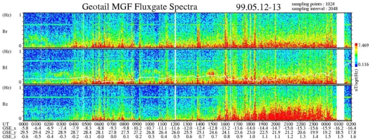
Fig. 10.Same as Fig. 9 but for 11 May 1999.
spin plane. This satellite coordinate system is close to the geocentric solar ecliptic (GSE) coordinate system, with the spin axis subtending an angle of 87◦ to the ecliptic plane. The data are then transformed to a field-aligned coordinate system. In this system theZ axis is parallel to the ambient magnetic field, theY axis is defined as the cross product of the unit vector in the direction of the spin axis and that in the direction of the ambient magnetic field, and theX axis is defined by the cross product of unit vectors along theY
andZaxes. The right-hand and left-hand components of the magnetic field are defined as follows
BXcos(ωt+φBX)+iBYcos(ωt+φBY)
=Brexp(iωt+φBr)+Blexp(−iωt+φBl) (1) whereBX andBY are amplitudes of theX and Y com-ponents in the field-aligned system;Br andBl are the
am-plitudes of the right-hand and left-hand components, respec-tively; andφBX,φBY,φBr, andφBlare phases for each com-ponent, respectively. The compressional component corre-sponds to theZcomponent in the field-aligned system.
From 16:40 UT (10), when the bow shock was crossed, to 21:00 UT (10), wave power resides in both the compressional and transverse (to the background field) directions. Up to 19:00 UT (10) power is intermittently present up to frequen-cies of ∼1 Hz (for comparison, the proton gyrofrequency here is∼0.18 Hz), an upward shift in the frequency presum-ably due to the Doppler shift induced by the flow speed. Af-ter 21:00 UT, the compressional power fades slowly away (see also Fig. 6, bottom panel) and the frequency spectrum becomes dominated by left-handed transverse activity. This transverse activity continues until 12:00 UT (11). After
Fig. 11.Same as Fig. 9 but for 12 May−02:00 UT, 13 May 1999.
(Fig. 2) the left-hand power drops out, leaving only sporadic bursts of weak right-hand activity. This transition correlates well with significant values of|Ap|, withAp<0 (Fig. 6).
On 12 May (Fig. 11c), as the density is recovering in the second solar wind regime, transverse and compressional wave activity resume between 04:00–09:00 UT. The bow shock is gaining in strength, increasing the perpendicular temperature and thereby the positive temperature anisotropy (Sckopke et al., 1990). During this period there are close counters with magnetopause/LLBL. Indeed, during the en-tries identified above at 06:00 UT and 09:00 UT, the wave activity subsides, and in the second crossing drops out com-pletely. Intense wave activity in all components resumes at
∼16:00 UT (12) with a predominance of the compressional power. This is the time when normal magnetosheath condi-tions prevail, as may be seen in the time series (Fig. 5).
Summarizing, during the density dropout (MHD– dominated magnetosheath), the magnetosheath is bereft of waves, except for weak, sporadic, right-hand activity. In par-ticular, compressional power in the main body of the mag-netosheath is completely absent, the very reverse of what is typically seen at the dayside (Anderson et al., 1991, 1993) and on the flanks (Lucek et al, 1999, Farrugia et al., 2000b). Normal magnetosheath wave activity is present in the last 9– 10 h of the pass. We now discuss the wave observations from the viewpoint of the linear kinetic theory of electromagnetic ion waves.
4 Magnetosheath waves: theory
The theory of electromagnetic ion waves is based on modes varying asexp(−iωt+ik·x), where a real wavevectork is given, and ω=ωr+iγ is in general complex valued. The real partωr=ℜ(ω) is the angular frequency in rad s−1 of the mode, while the imaginary partγ=ℑ(ω)is the growth (damping) rate of the wave according asγ >0(<0). Thus
τe=1/γ gives the corresponding e-folding time in s.
Quan-tity ω is computed from a dispersion relation of the form
D(ω,k, Q)=0 that contains a set of plasma parametersQ. This equation, derived from kinetic theory (see, e.g. Gary, 1993), is usually set up in the plasma frame. The waves can be excited by instabilities, depending on the values of the parametersQ.
In the frequency rangeωr≤p(the proton gyrofrquency), three wave modes were observed by Geotail in the magne-tosheath, all of which are driven byAp. Their intensity and other physical characteristics vary in concert with changes inAp andβp, and are also Doppler-shifted by the flowV, which near the dusk terminator is appreciable, to a frequency
¯
ωr=ωr+k·V. The waves were: 1) the mirror modes (MMs) 2) left-hand polarized ion cyclotron waves (L-EICWs) and 3) right-hand polarized ion cyclotron waves (R-EICWs). As noted in the Introduction, the MMs are usually the dominant wave mode in the main body of the (normal) magnetosheath, but disappear in the PDL because of the lowβp prevailing in that region, see, e.g. (Schwartz et al., 1996). Because the R-EICWs are driven by a negativeAp, which is not usually the case in the magnetosheath, they are not ordinarily excited in the magnetosheath, and are observed there and in the PDL only as daughter waves, generated by nonlinear wave inter-actions in both regions.
Below we shall address the following points of the obser-vations:
1. In comparison with typical EICW intensities exempli-fied by those on 10 May, EICWs in the lowPdyn-low
MAmagnetosheath are present but at much reduced in-tensities;
2. Sometimes R-EICWs appear alone driven directly by negativeAp; and
We note that in the following calculations we omit the con-tribution of the α-particles. We thereby underestimate the theoretical excitation rates of both L- and R-EICWs, which are both enhanced by the presence ofα’s (see Gratton and Farrugia, 1996; Farrugia et al., 1998; Gnavi et al., 2000.) The same is true for MMs waves. The theory, therefore, gives only conservative estimates of the growth rates.
4.1 L-EICWs
The instability of L-EIC waves is due to positiveAp. These modes grow when the protons resonate with the waves, i.e. when condition
ωr−kvk=p (2)
is satisfied. Here,vk is the particle velocity parallel to the magnetic field. Waves propagating alongB, i.e. withk⊥=0 andk=kk, are amplified faster, and we shall assume that the observed waves are mainly of this kind. We consider only protons. We shall also assume a bi-Maxwellian distribution,
fBMax0 =
1
π
3/2 1
vthkv2th⊥
exp −(vk)
2
vth2k
!
exp −(v⊥)
2
vth2⊥)
!
, (3)
wherevt h,k,⊥≡√(2KBTk,⊥/mp).
It is convenient to normalize as follows:
x=ω/ p, xr =ωr/ p, y=kVA/ p, g=γ / p.(4)
The resonant protons move against the wave (i.e. withvk<0 when the phase velocity vph>0), so that resonance occurs for waves with xr<1. At resonance (Eq. 2), wave emis-sion or wave absorption may take place. However, when
xr is less than a critical value xc≡Ap/(Ap+1), emission is the dominant process and the wave grows, while for
xr>xc, absorption prevails. From equations 2–4 it
fol-lows that the fraction of resonant protons is proportional to
exp(−(1/βp,k)((xr−1)/y))2)(see, e.g. Gnavi et al., (2000),
Farrugia et al. (2004), and references therein) and is thus reg-ulated byβp,k≡(vt h,k/VA)2, decreasing asβp,kdecreases.
During May 11, 1999, L-EIWC activity was greatly cur-tailed by two factors: 1) the large decrease ofβp, which re-duced the emission rate per particle, and 2) the strong de-crease of the density which, in turn, reduced the number of emitters. Both effects are taken into account in the nor-malized growth rate,g, computed by solving for each realy
the dispersion equation of L-EICWs forx(see, for instance, Gratton and Farrugia, 1996)
y2=Ap−x+
(Ap+1)x−Ap
ypβk,p
Z x−1
ypβk,p
!
. (5)
Z is the plasma dispersion function. In view of the fact that the electrons have only a minor influence on L-EICWs we have neglected the inertia of electrons and assumed that
Ae=0 in (eq.5). (Wind/SWE values ofAelie in the interval -0.5≤Ae≤0.5 with large scatter).
Using experimental values of Ap and
βk,p=(3Tk/(2T⊥+Tk))βp, we solve Eq. 5 with param-eters changing with time. The normalized growth rates g
are shown as a function of the Doppler-shiftedxr in the 3-D plots of Figs. 12 and 13. Time is the third axis and increases towards the left. Data for the calculations are available only where there is a horizontal line segment starting at the UT axis. When the horizontal line segment extends along the wholexr range the correspondingg<10−4. From
∼21:00 UT (11) to∼04:00 UT (12) there is a gap in theAp data and growth rates are not computed (blank in Fig. 13). The shift in frequency is computed and plotted only for forward-propagating wavesvph>0 using the angle between
VandBshown in the last panel of Fig. 5. We shall comment later about the Doppler shift of backward-propagating waves, which correspond to roots of the dispersion equation for negative y values that are equally amplified. We can see that the frequency range of amplified waves goes intermittently beyond the proton gyrofrequency (at xr=1 here, andfp in the spectrograms), as also observed in the spectrograms of Figs. 9 and 10, though experimental values are somewhat higher. Evidently there could be no agreement between theoretical and observed frequencies without taking into account the important Doppler shift at the spacecraft position.
The normalized frequency for which the theory predicts a maximum growth rate for L-EICWs is shown as a function of time in the upper panel of Fig. 14. The thin line join-ing plus symbols, computed with experimental data, is the frequency in the plasma frame, while the thick line joining diamond symbols corresponds to Doppler-shifted values for
vph>0. The latter are about a factor of 2–3 higher than the former. The lower panel in Fig. 14 gives the correspond-ing normalized maximum growth rates as a function of time. The wide gap in computed properties, from∼13:00 UT (11) to∼04:00 UT (12) is due to the growth rates being less than 10−4because of lowAp and/or lowβp,k, or absence of L-EICWs amplification due to negativeAp, during the first part of the interval (up to∼21:00 UT (11)), and for the rest of the period is due to the data gap noted above. A growth rate
g=10−4is very weak, meaning that∼1600 proton gyrope-riods have to elapse before the wave amplitude increases by a factore≃2.72.
Starting from Fig. 12 at 18:00 UT (10), theory shows EICWs amplification at ∼ 20:00 UT (10) followed by negligible g values until a stronger excitation occurs at
∼21:00 UT (10), a time in whichAp(>0) increases signif-icantly (Fig. 6). The theoretical amplification is then mod-ulated according to the variations ofAp−βp (Fig. 6), with varying values ofgfrom∼21:00 UT (10) to∼05:00 UT (11), when a short data gap appears. Additional modulations con-tinue from∼06:00 UT (11) to∼10:00 UT (11), after which the excitation becomes negligible. We may note peaks of amplification, withgbetween 0.01 to 0.1 at∼21:00 UT (10),
∼02:00 UT (11),∼04:00–05:00 UT (11),∼06:00 UT (11),
reduced wave excitation.
The absence of wave amplification from shortly after
∼11:00 UT (11) to after ∼20:00 UT (11) seen in Figs. 9 and also Fig. 14 is, according to the theory, a consequence of the long interval dominated by negativeApvalues, which prevented the excitation of L-EICWs (Fig. 6, panel 4). When positiveAp were sporadically observed in this interval, the concomitant low beta was not sufficient to produceg>10−4. Figure 13, which is a continuation of Fig. 12, covers the period from 12:00 UT (11) to 20:00 UT (12). Here the am-plification reappears at∼04:00 UT (12), after the data gap. The growth rate rises to a peakg∼0.1 at∼05:00 UT (12), it is negligible from∼07:00–08:00 UT (12), grows again to sub-stantial values from∼09:00–11:00 UT (12), falls down after
∼11:00 UT (12) and peaks strongly again at 12:00 UT (12). Therafter follows a valley of very lowgup to∼15:00 UT (12), then some additional peaks at∼15:00–16:00 UT (12), and at∼17:00 UT (12), after which the theoretical amplifi-cation becomes negligible.
After about 18:00 UT (12), during the high MA phase brought about by the recovery of the density, the compres-sional activity observed in the spectrograms (which restarted some hours earlier) becomes stronger and keepsAp at low values, as shown in Fig. 6. The smallApvalues, in turn, re-duce the growth rate of the L-EICWs to negligible values, as shown in Figs. 10 and 11, so that we do not extend Fig. 13 beyond 20:00 UT (12).
4.2 R-EICWs
The R-EICWs are observed sometimes together with L-EICWs, and at other times alone (Figs. 9, 10 and 11). These two cases have to be treated separately.
According to linear theory, an instability of the R-EICWs can be excited by a negative temperature anisotropy, pro-vided theβpis not too small, (see (Gary, 1993). At the same time, a negativeAp inhibits the growth of the L-EICWs, as noted above. According to the linear theory R-EIC waves are not amplified at all whenAp>0. When R-EICWs are observed underAp>0 conditions, they are by-products of L-EIC waves (see, for example, last part of 10 May and early part of 11 May). Note also that whenAp>0 andβp≤1 the R-EICWs have little or no damping, particularly atxr<1, so they may last long after being generated. Conversely, when
βpis large the damping of R-EICWs may increase consider-ably, except at very low frequencies,xr≪1.
We consider now the case of negative Ap. Geotail ob-serves weak bursts of R-EICWs with little accompanying L-EICWs (Fig. 10). These right-hand waves are now be-ing generated directly from the temperature anisotropy. In-terestingly, this period coincides with a weak bow shock so that the magnetosheath is exposed to the proton temperature anisotropy of the solar wind. This is negative (see Fig. 2, panel 5). We conclude that this weak R-EICW activity is di-rectly a result of the weakening of the bow shock, thus elim-inating a major source for preferentially enhancingT⊥at the expense of theTk(Sckopke et al., 1990).
0 0.5 1 1.5 18 (10) 20 (10) 22 (10) 00 (11) 02 (11) 04 (11) 06 (11) 08 (11) 10 (11) 12 (11) 10−4 10−3 10−2 10−1 x rDopp UT g
Fig. 12. Theoretical results on L-EICWs using measured values at
Geotail. Plotted are the growth rates,gin units ofp, against UT
and Doppler−shifted frequeciesxr normalized top. The time
axis is in hours starting from 18:00 UT, 10 May 1999, and increases to the left. This interval starts soon after the bow shock crossing and ends at the lowest values of the solar wind density 12:00 UT (11). Left-hand-amplification with modulations ingthroughout the interval except for 2 h at its extremities.
0 0.5 1 1.5 2 16 (11) 16(12) 20 (11) 24 (11) 04 (12) 08 (12) 12 (12) 12 (11) 10−4 10−3 10−2 10−1 xrDopp UT g
Fig. 13. Same as Fig. 9, but for the interval 12:00 UT (11) to
20:00 UT (12), i.e. during the phase when the density starts to recover. Note the absence of L-EICW amplification in the inter-val 12:00 UT (11) to 04:00 UT (12), in agreement with the data (Fig. 10).
The R-EICW activity observed in the interval after
∼12 UT (11) and∼21:00 UT (11) whenAp<0 corresponds to very low valuesβp (<0.1), but we must note that βp,k, which is the key parameter for the waves, was>0.1 due to the sporadically enhanced, negative anisotropy. As an example of the theoretical results, we quote two computations, one for
∼12:00 UT (11) and the other for 15:00–16:00 UT (11). (For the dispersion relation see, for example Farrugia et al., 1998). For the first we haveβp=0.09 andAp=-0.8, andβp,k=0.19. For the second we haveβp=0.09,Ap=−0.94,βp,k=0.24. In both cases we findg≈0.1 in the frequency range 0.35–0.37
2-18 (10) 24 (10) 06 (11) 12 (11) 18 (11) 24 (11) 06 (12) 12 (12) 18 (12) 24 (12) −0.4 −0.2 0 0.2 0.4 0.6 0.8 1 1.2 UT xr, xr Dopp
18 (10) 24 (10) 06 (11) 12 (11) 18 (11) 24 (11) 06 (12) 12 (12) 18 (12) 24 (12) 10−4 10−3 10−2 10−1 UT g
Fig. 14. Theoretical maximum growth rates of L-EICWs (bottom
panel) and corresponding frequencies (upper panel) for the interval 18:00 UT (10)–24:00 UT (12), where data for the computations are available. Note that at dusk there is a large Doppler shift in the frequency (thick line) due to the fast magnetosheath flow at dusk. In the gap the temperature anisotropyAp<0, and these waves are
not excited.
3 as before, it yields forvph>0 a frequency∼p. Outside the cited frequency range the growth rate becomes very small because|Ap|is small. These estimates are in agreement with the observed weak right-handed emission whenAp<0.
The weakness of the R-EICW power at this time may be explained as follows. The amplification of R-EICWs is due to the cyclotron resonance of ions with the waves:
ωr−kvk= −p, (6)
which is known as the anomalous resonance condition. Equation (eq-6) is satisfied only whenvk>vph, and for these wavesvph>VA. Therefore, under this condition, and remem-bering thatβp,k=(vt h,k/VA)2, it follows that there are only few particles in the proton distribution function that travel faster than the R-EIC waves when βp,k≪1 and resonate, sincevph>VA>vt h. Therefore, asβp,kdecreases due to an increase ofVAat nearly constant temperature, the R-EICWs excitation is reduced.
4.3 Mirror mode waves
The mirror modes have a wavevector quasi-perpendicular to the field (k⊥≫kk,k≈k⊥). A characteristic signature of the MMs is the anticorrelation of magnetic field fluctuations with density perturbations. The condition for the MMs instability resulting from kinetic theory is
1−X s
(β⊥,sAs) ≤ 0, (7)
where the sum extends over all the particle species (see, e.g. Hasegawa, 1975; Treumann and Baumjohann, 1997).
Taking only protons into account, we represent the theoret-ical instability limit (Eq. 7) by a horizontal line in last panel
of Fig. 6. The points represent experimental values. The quantityβpand the temperature ratios are 1-min running av-erages. The mirror instability is a non–resonant process in which all the particles participate, and it tends to reduce the anisotropy as the amplitude of the waves grows. Therefore, these modes are ordinarily only marginally unstable, and are observed close to the theory limit.
4.4 Comparison of wave theory with the observed spectra A general preliminary comment: the linear theory of waves cannot reproduce fully the observed power spectrum, due to the absence of wave-wave interactions and other realistic elements omitted in the treatment. Nevertheless, the linear model can point out some basic trends of the wave activity, predict the presence or absence of the instability, and reveal the influence on the waves of the variation of important phys-ical parameters. With these limitations in mind, we carry out a qualitative comparison of the theoretical properties com-puted with the observed wave phenomena.
Between∼21:00 UT (10) and 11:00 UT (11) a qualitative agreement between the observed spectral activity (Figs. 9, 10) and the computed frequencies and amplification rates can be noted. (see Figs. 12 and 14) At about 21:00 UT (10), when the mirror mode activity declines significantly, the parame-terAp increases and, correspondingly, the growth rates of L-EICWs expected from linear theory reach substantial val-ues (Fig. 12). Note also in Figs. 9–10 the observed relative reduction of L-EICWS activity at about and after 24:00 UT (10), a recovery from 02:30 to 04:30 UT (11), a decline from 05:00 UT (11) to 07:00 UT (11), followed by a weak revival at low frequencies from 07:00 UT (11) to 11:00 UT (11), and the subsequent fade out. These features are qualitatively re-flected in Figures 12 and 14 as trends of growth rate variation, at approximately the same times.
The observed intensity at very low frequencies, with
ω≪p in the range f<0.1 Hz (Figs, 9, 10 and 11) can be explained within the linear theory by the amplification of backward-propagating L-EICWs (vph<0). For these waves, which propagate against the field,kkis replaced by -kk, and the observed resonant frequency is, therefore,ω¯r=ωr−|k|V (Eq. 2) so that the Doppler shift may reduce their frequency considerably. An additional, different, contribution to the L-EIC wave population at low frequency may be non-linear interactions producing a cascade from the excited frquency range down to lower frequencies.
A temporary absence of theoretical L-EICW growth rate may be noted at∼09:00 UT (12), Fig. 13, at the same time of a transient entry of Geotail into the magnetosphere, discussed before, when a power decline appears in the spectrogram of Fig. 11.
The presence of R-EICWs under positive temperature anisotropy conditions seen in the spectrograms can be explained by the linear theory, from the Doppler shift of already existing backward propagating L-EICWs, or those excited together with forward propagating L-EICWs when
increase the frequency of L-EICWs withvph>0 by factors varying from 2–3. For vph<0, negative values of ω¯r are also obtained, which means that Doppler-shifted, backward propagating L-EICWs can be observed as R-EICWs. The recorded R-EICWs may also be generated, at least in part, by nonlinear wave interactions that can produce these modes from pre-existing L-EIC waves.
Theory predicts no wave amplification from∼11:00 UT (11) to∼21:00 UT (11) (Figs. 12–13), a long interval where availableApdata shows a preponderance of negative values, which prevent the growth of L-EIC waves. The same time period is characterized by a sharp decline, and almost ab-sence of L-EICW power, except for a trace at very small fre-quencies (Fig. 11). This is also the period of observed weak bursts of R-EICWs power, in agreement with theoretical no-tions about R-EICWs excitation whenAp<0. The R-EICW bursts occur at about 12:00 UT (11), 14:00 (11), 16:00 (11), 18:00 (11), 20:00 (11), and 21:00 UT (11). As noted, this activity cannot be a by-product of L-EICWs excitation.
The agreement between the theoretical instability limit of Fig. 6 and the MMs activity shown in the spectrograms of Figs. 9–11 is, in general, good during the whole interval studied, taking into account the fact that mirror modes are ordinarily only marginally unstable, as mentioned in the In-troduction and Sect. 4.3. This comment applies also to some details of the spectrograms. For instance, one may note the MM bursts at∼21:00 UT (10), and at∼06:00 UT (12) that can be correlated with points lying on, or above, the theoret-ical instability limit at the same times.
To conclude, not all the observed spectral features can be explained by the linear theory. An example of the lat-ter discrepancy is the L-EICW activity seen in Fig. 11 af-ter∼18:00 UT (12). Furthermore, the critical quantityAp is not easily measured, and has been 1 min averaged. Nev-ertheless we have been able to point out several qualitative, sometimes even quantitative, agreements between theory and experiment.
5 Conclusion
We have presented observations of magnetosheath field, plasma, and, most of all, wave properties during very un-usual conditions. We now highlight what, in our view, is the significance of the reported results on our knowledge of the magnetosheath. The major extreme element was the very low solar wind dynamic pressure. This had two consequences. This first is that, because at the same time the magnetic field strength remained fairly constant, the solar wind Alfven Mach number was also low. The latter implies that mag-netosheath properties were controlled strongly by the IMF, which means that the magnetosheath was essentially PDL-like. An expectation of both theory and observations con-cerning this regime is that there should be transverse wave activity, EICWs. In fact, these were observed. Thus we have verified a theoretical expectation, and extended observational
work on electromagnetic ion waves in the magnetosheath to the low dynamic pressure regime.
The second consequence of low solar wind dynamic pressure is that the resulting Alfven (and magnetosonic) Mach number weakened the bow shock. The weak bow shock exposed the magnetosheath directly to the temperature anisotropy of the solar wind, which was negative. Plasma wave theory then predicts the presence of right-hand polar-ized EICWs, deriving their energy from the anisotropy. And these waves were observed. We have thus confirmed another prediction of wave theory in the context of space physics plasmas. To our knowledge, this is the first observation of transverse right-hand EICWs existing alone in the magne-tosheath.
The temporal aspect of the observations was very crucial in our case. As Fig. 3 clearly demonstrates, the solar wind underwent a large-scale transformation, and Geotail stayed long enough in the magnetosheath to observe its effect. In this case, clearly, what class of waves were observed de-pended on a temporal feature and did not reflect a spatial structure of the magnetosheath. As a corollary, the waves observed were not related to the position of the spacecraft with respect to the magnetopause or bow shock: EICWs were seen in the main body of the magnetosheath, without mirror waves; and mirror mode waves were observed right next to the magnetopause.
Acknowledgements. Part of this work was done while FTG and GG were on research visits at the Space Science Center of the Univer-sity of New Hampshire. We thank T. Nagai for kindly providing the magnetic field data from Geotail. Geotail data are courtesy of the DARTS website at http://www.darts.isas.ac.jp. This work is sup-ported in part by NASA Grants NAG5-12189, and NAG5-13116, NASA Wind Grant NAG5-11803, and the Argentinian UBACyT grant X032 and CONICET PIP 2013/01.
Topical Editor T. Pulkkinen thanks C.-H. Lin for his help in evaluating this paper.
References
Abraham-Shrauner, B.: Determination of magnetohydrodynamic shock normals, J. Geophys. Res., 77, 736–739, 1972.
Anderson, B. J. and Fuselier, S. A.: Magnetic pulsations from 0.1 to 4 Hz and associated plasma properties in the Earth’s subsolar magnetosheath and plasma depletion layer, J. Geophys. Res., 98, 1461–1480, 1993.
Anderson, B. J., Fuselier, S. A., and Murr, D.: Electromagnetic ion cyclotron waves observed in the plasma depletion layer, Geo-phys. Res. Lett., 18, 1955–1958, 1991.
Anderson, B. J. Fuselier, S. A., Gary, S. P., and Denton, R. E.: Mag-netic spectral signatures in the Earth’s magnetosheath and plasma depletion layer, J. Geophys. Res., 99, 5877–5892, 1994. Erkaev, N. V. : Results of the investigation of MHD flow around the
magnetosphere, Geomagn. Aeron., 28, 455–464, 1988.
Fairfield, D. H., Cairns, I. A., Desch, M. D., Szabo, A., Lazarus, A. J., and Aelig, M. R.: The location of low Mach number bow shocks at Earth, J. Geophys. Res., 106, 25 361–25 376, 2001. Farrugia, C. J., Erkaev, N. V., Biernat, H. K., and Burlaga, L. F.:
Anomalous magnetosheath properties during Earth’s passage of an interplanetary magnetic cloud, J. Geophys. Res., 100, 19 245– 19 258, 1995.
Farrugia, C. J., Gratton, F. T., Gnavi, G., and Ogilvie, K. W.: On the possible excitation of electromagnetic ion cyclotron waves in ejecta, J. Geophys. Res., 103, 6543–6550, 1998.
Farrugia, C. J., Singer, H. J., Evans, D. S., Berdichevsky, D., Scud-der, J. D., Ogilvie, K. W., Fitzenreiter, R. J., and Russell, C. T.: Response of the equatorial and polar magnetosphere to the very tenuous solar wind on 11 May 1999, Geophys. Res. Lett. 27, 3773–3776, 2000a.
Farrugia, C. J., Gratton, F. T., Contin, J., Cocheci, C. C., Arnoldy, R. A., Ogilvie, K. W., Lepping, R. P., Zastenker, G. N., Noz-drachev, M. N., Fedorov, A., Sauvaud, J.-A., Steinberg, J. T., and Rostoker, G. : Coordinated Wind, Interball/tail, and Ground observations of Kelvin-Helmholtz Instability and Waves in the near-tail, equatorial magnetopause at dusk: 11 January 1997, J. Geophys. Res., 105, 7639–7668, 2000b.
Farrugia, C. J., Gnavi, G., Gratton, F. T., Matsui, H., Torbert, R. B., Lepping, R. P., Oieroset, M., and Lin, R. P.: Electromagnetic ion cyclotron waves in the subsolar region under normal dynamic pressure: Wind observations and theory, J. Geophys. Res., 109, doi: 10.1029/2003JA010104, 109, 2004.
Gary, S. P.: Theory of Space Plasmas Microinstabilities, Cambridge University Press, New York, 1993.
Gary, S. P. and Lee, M. A.: The ion cyclotron anisotropy instability and the inverse beta correlation between proton anisotropy and proton beta, J. Geophys. Res., 99, 11 297–11 302, 1994. Gary, S. P., McKean, M. E., Winske, D., Anderson, B. J., Denton,
R. E., and Fusilier, S. A. : Proton cyclotron anistropy instability and the anisotropy/beta inverse correlation, J. Geophys. Res., 99, 5903–5914, 1994.
Gnavi, G., Gratton, F. T., and Farrugia, C. J.: Theoretical properties of electromagnetic ion cyclotron waves in the terrestrial, dayside, low latitude plasma depletion layer under uncompressed magne-tosheath conditions, J. Geophys. Res., 105, 20 973–20 988, 2000. Gratton, F. T. and Farrugia, C. J., Electromagnetic ion cyclotron waves in the terrestrial plasma depletion layer: Effects of possi-ble relative motion between H+ and He2+ions, J. Geophys. Res., 101, 21 553–21 560, 1996.
Hasegawa, A.: Plasma Instabilities and Non Linear Effects, Springer Verlag, New York, 1975.
Hill, P., Paschmann, G., Treumann, R. A., Baumjohann, W., and Sckopke, N. : Plasma and magnetic field behavior across the magnetosheath near local noon, J. Geophys. Res., 100, 9575– 9584, 1995.
Kasaba, Y., Terasawa, T., Tsubouchi, K., Mukai, T., Saito, Y., Mat-sumoto, H., et al. : Magnetosheath electrons in anomalously low density solar wind observed by Geotail, Geophys. Res. Lett., 27, 3253–3256, 2000.
Kivelson, M. G. and C. T. Russell, (Eds) : Introduction to Space Physics, Cambridge University Press, New York, 1995. Kokubun, S., Yamamoto, T., and Acuna, M. H., et al.: The Geotail
Magnetic Field Experiment, J. Geomag. Geoelectr., 46, 7–21, 1994.
Lees, L.: Interaction between the solar wind plasma and the geo-magnetic cavity, AAIA J, 2, 1576–1582, 1964.
Lepping, R. P., Acuna, M. H. and Burlaga, L. F., et al.: The
Wind Magnetic Field Investigation, Space Sci. Rev., 71, 207– 229, 1995.
Lucek, E. A., Dunlop, M. W., Balogh, A., Cargill, P., Baumjohann, W., Georgescu, E., Haerendel, G., and Fornacon, H.-K.: Identi-fication of magnetosheath mirror modes in Equator-S magnetic field data, Ann. Geophys., 17, 1560–1573, 1999.
Matsui, H., Farrugia, C. J., and Torbert, R. B.: Wind-ACE solar wind correlations, 1999: An approach through spectral analysis, J. Geophys. Res., 1355, doi:10.1029/2002JA009251, 107, 2002. Midgley, J. E. and Davis, L.: Calculation by a moment technique of the perturbation of the geomagnetic field by the solar wind, J. Geophys. Res., 68, 5111–5123, 1963.
Mead, G. D. and Beard, D. B. : Shape of the geomagnetic field solar wind boundary, J. Geophys. Res., 69, 1169–1179, 1964. Mukai, T., Machida, S., and Saito, Y., et al.: The Low-Energy
Par-ticle (LEP) Experiment onboard the Geotail satellite, J. Geomag. Geoelectr., 46, 669–692, 1994.
Nakagawa, T., Nishida, A., and Saito, T.: Planar magnetic structures in the solar wind, J. Geophys. Res., 94, 11 761–11 775, 1989. Ogilvie, K. W., Chornay, D. J., and Fitzenreiter, R. J., et al.: SWE, A
comprehensive plasma instrument for the Wind spacecraft, Space Sci. Rev., 71, 55-77, 1995.
Phan, T.-D., Paschmann, G., Baumjohann, W., Sckopke, N., and Luehr, H.: The magnetosheath region adjacent to the dayside magnetopause: AMPTE/IRM observations : J. Geophys. Res., 99, 121–142, 1994.
Richardson, J. D. and Paulerena, K. I.: Plasma and magnetic field correlations in the solar wind, J. Geophys. Res., 103, 239–252, 2001.
Schwartz, S. J., Burgess, D., and Moses, J. J.: Low-frequency waves in the Earth’s magnetosheath: present status, Ann. Geophys., 14, 1134–1150, 1996,
SRef-ID: 1432-0576/ag/1996-14-1134.
Shue, J.-H., Song, P., Russell, C. T., Steinberg, J. T., Chao, J. K., Za-stenker, G., Vaisberg, O. L., Kokubun, S., Singer, H. J., Detman, T. R., Kawano, H.: Magnetopause location under extreme so-lar wind conditions, J. Geophys. Res., 103(A8), 17 691–17 700, 1998.
Sckopke, N., Paschmann, G., Brinca, A. L., Carlson, C. W., and Luehr, H. : Ion thermalization in quasi-perpendicular shocks in-volving reflected ions, J. Geophys. Res., 95, 6337–6352, 1990. Song, P., Russell, C. T., and Thomsen, M. F.: Slow mode
transi-tion in the frontside magnetosheath, J. Geophys. Res., 97, 8295– 8305, 1992.
Sonnerup, B. U. O.: The reconnecting magnetopause, in: Magneto-spheric Physics, (Ed) McCormac, B. M., 23–33, D. Reidel, Nor-well, Mass., 1974.
Sonnerup, B. U. O.: Theory of the low-latitude boundary layer, J. Geophys. Res., 85, 2017–2026, 1980.
Sonnerup, B. U. O. and Cahill, L. J.: Magnetopause structure and attitude from Explorer 12 observations, J. Geophys. Res., 72, 171–183, 1967.
Sonnerup, B. U. O and Siebert, K. D.: Theory of the low-latitude boundary layer and its coupling to the ionosphere: A tutorial re-view, in: Earth’s Low-Latitude Boundary Layer, (Ed) Newell, P. T., and Onsager, T., Geophys. Monograph 133, AGU, 13–32, 2003.
Spreiter, J. R. and Alksne, A. Y.: Plasma flow around the magneto-sphere, Rev. Geophys., 7, 11–50, 1969.
Spreiter, J. R. and Stahara, S.: A new predictive model for determin-ing solar wind-terrestrial planet interaction, J. Geophys. Res., 85, 6769–6777, 1980.
Terasawa, T., Kasaba, Y., Tsubouchi, K., Mukai, T., Saito, Y., Frank, L. A., et al.: Geotail observations of anonalously low density solar wind in the magnetosheath, Geophys. Res. Lett., 27, 3781–3784, 2000.
Treumann, R. A. and Baumjohann, W.: Advanced Space Plasma Physics, Imperial College Press, 1997.
Wang, Y. L., Raeder, J., Russell, C. T., Phan, T. D., and Manapat, M.: Plasma depletion layer: Event studies with a global model, J. Geophys. Res., doi:10.1029/2002JA009281, 108, 2003. Zwan, B. J. and Wolf, R. A.: Depletion of the solar wind plasma