WIND observations of coherent electrostatic waves in the solar wind
A. Mangeney1, C. Salem1, C. Lacombe1, J. -L. Bougeret1, C. Perche1, R. Manning1, P. J. Kellogg2, K. Goetz2, S. J. Monson2, J. -M. Bosqued3
1URA 264 du CNRS, DESPA, Observatoire de Paris, 92195 Meudon, France
2School of Physics and Astronomy, University of Minnesota, Minneapolis, MN 55454, USA 3CESR/CNRS, Universite Paul Sabatier, BP 4346, 31029 Toulouse, France
Received: 15 June 1998 / revised: 14 September 1998 / Accepted: 15 September 1998
Abstract. The time domain sampler (TDS) experiment on WIND measures electric and magnetic wave forms with a sampling rate which reaches 120 000 points per second. We analyse here observations made in the solar wind near the Lagrange point L1. In the range of frequencies above the proton plasma frequency fpi and
smaller than or of the order of the electron plasma frequencyfpe, TDS observed three kinds of electrostatic
(e.s.) waves: coherent wave packets of Langmuir waves with frequencies f 'fpe, coherent wave packets with
frequencies in the ion acoustic range fpif <fpe, and
more or less isolated non-sinusoidal spikes lasting less than 1 ms. We con®rm that the observed frequency of the low frequency (LF) ion acoustic wave packets is dominated by the Doppler eect: the wavelengths are short, 10 to 50 electron Debye lengths kD. The electric
®eld in the isolated electrostatic structures (IES) and in the LF wave packets is more or less aligned with the solar wind magnetic ®eld. Across the IES, which have a spatial width of the order of'25kD, there is a small but
®nite electric potential drop, implying an average electric ®eld generally directed away from the Sun. The IES wave forms, which have not been previously reported in the solar wind, are similar, although with a smaller amplitude, to the weak double layers observed in the auroral regions, and to the electrostatic solitary waves observed in other regions in the magnetosphere. We have also studied the solar wind conditions which favour the occurrence of the three kinds of waves: all these e.s. waves are observed more or less continuously in the whole solar wind (except in the densest regions where a parasite prevents the TDS observations). The type (wave packet or IES) of the observed LF waves is mainly determined by the proton temperature and by the direction of the magnetic ®eld, which themselves depend on the latitude of WIND with respect to the heliospheric current sheet.
Key words. Interplanetary physics (plasma waves and turbulence; solar wind plasma). Space plasma physics (electrostatic structures).
1 Introduction
Electrostatic waves with frequenciesf between the ion and electron plasma frequenciesfpif <fpe have been
studied for more than 20 years in the inner heliosphere (see the Helios observations and a comparison with the Pioneer observations, Gurnett and Anderson, 1977). Their wavelengthkis of the order of a few tens of Debye lengthskD(Gurnett and Frank, 1978), their electric ®eld
E is very closely aligned with the local magnetic ®eld, and the corresponding electric energy density is small compared to the thermal energy density of the plasma: indeed,0E2= 2NkBTeis only about 10ÿ7to 10ÿ5during
intense bursts, and much smaller on the average (Gurnett, 1991). (0, vacuum dielectric constant; N,
particle number density; kB, Boltzmann constant; Te,
temperature of the electrons).
Initially observed with instruments having relatively poor time and frequency resolution, they appeared as very bursty broad band emissions lasting from a few hours to a few days. Observations made with higher time resolution (Kurth et al., 1979) revealed that the emissions were actually formed of brief narrow band bursts with rapidly drifting center frequency.
This electrostatic activity occurs quite frequently but is not a permanent feature of the solar wind. Gurnett et al. (1979) found that the greatest intensity and frequency of occurrence was observed in the slow speed wind where Vsw500 km/s and the electron
tempera-ture Te is larger than the proton temperature Tp.
However, substantial wave intensities are also observed for high speed ¯ows and small temperature ratio, Te=Tp '0:3. The wave intensity decreases with
ing distance from the sun and seems to be correlated with the parameters which measure the deviations of the particle distributions from Maxwellian ones (such as the electron heat ¯ux or the quality of the ®t of proton distributions by a Maxwellian).
The URAP instrument onboard Ulysses observed waves in the fpif <fpe frequency band even at high
heliographic latitudes. However, the regions with the most intense ion acoustic (IAC) wave activity were found at low heliographic latitudes (MacDowall et al., 1996).
Neither the wave modes nor the source of these waves have yet been unambiguously identi®ed (see Gurnett, 1991). Gurnett and Frank (1978) proposed that they were ion acoustic waves propagating along the ambient magnetic ®eld, with frequencies f0 lower than
the local ion plasma frequencyfpi in the plasma frame,
but strongly Doppler shifted to the observed range in the spacecraft frame. Several instabilities have been suggested to be responsible for their occurrence. For example, the electron heat ¯ux (Forslund, 1970; Dum et al., 1981) may be a source of free energy for the e.s. IAC mode. But Gary (1978) has shown that other, electromagnetic, heat ¯ux instabilities have much larger growth rates in conditions typical of the solar wind. Another attractive possibility would be ion beams (Gary, 1978; Lemons et al., 1979; Marsch, 1991) such as those observed more or less continuously in the fast solar wind and drifting with roughly the local AlfveÂn speed with respect to the core ion distribution. These ion beams could excite IAC waves. However, Gary (1993) concludes that for the range of temperature ratios Te=Tp5 usually observed in the solar wind the
instability threshold is never reached.
Bursts of Langmuir waves (atfpe), not related to type
III solar bursts, have also been observed in the solar wind (Gurnett and Anderson, 1977; Gurnettet al., 1979); they are frequently associated with magnetic holes (Linet al., 1995a); their intensity appears to be signi®cantly higher at high heliographic latitudes (i.e. in the fast speed wind) than at low latitudes (MacDowallet al., 1996).
We shall describe here new observations by the time domain sampler (TDS) experiment which is part of the WAVES investigation on the WIND spacecraft. These observations were obtained in the ecliptic plane when WIND was at a distance of the Earth greater than 200 RE, near the Lagrange pointL1. These observations are
similar to those analysed by Kurthet al.(1979) but have a higher time resolution, up to 120 000 points per second. At this temporal resolution and in the unper-turbed (by the Earth) solar wind, the wave forms recorded by the TDS are coherent and display three typical shapes. Two of them correspond to wave forms already known: modulated wave packets at the Lan-gmuir frequency, and modulated wave packets with centre frequencies f in the IAC wave range (fpif <fpe) which will be called the low frequency
(LF) range in the following. The third type of wave form, which has not been previously reported in the free solar wind, consists of isolated electrostatic structures (IES) similar in many respects to those observed in
dierent regions of the Earth's environment (Temerin et al., 1982, Matsumotoet al., 1994, Mottezet al., 1997). We shall also discuss some observations indicating that this last type of wave form occurs in the vicinity of the L1 Lagrange point for all solar wind conditions, while the frequency of occurrence of the LF wave packets decreases with increasing distance from the heliospheric current sheet.
2 The data
The WAVES experiment on the WIND spacecraft measures the radio and plasma waves in a large range of frequencies, from a fraction of a Hertz up to 14 MHz for the electric ®eld, and up to 3 kHz for the magnetic ®eld (Bougeretet al., 1995).
In this study, we use the electric and magnetic wave form measurements from the time domain sampler (TDS) which is part of the WAVES package. This instrument uses two orthogonal antennas, the x-anten-na, a wire dipole of physical length 2Lx (Lx50 m)
tip-to-tip, and they-antenna, a much shorter dipole of physical length 2Ly (Ly 7:5 m) tip-to-tip. To obtain
the electric ®eldEalong thexoryantenna, we divide the measured electric potential dierenceV at the antenna terminals by the corresponding eective electric lengths
Lx or Ly. These eective electric lengths dier from the
physical ones due to the eects of the spacecraft environment; they are known within a few percent,
Lx41:3 m and Ly '0:1Lx. Since the signal-to-noise
ratio is usually smaller by an order of magnitude on the shorty-antenna than on the x-antenna we shall mainly use the data obtained with the x-antenna, except in Sect. 4.
The electromagnetic waveforms are organised as time series of 2048 data points, which will be calledeventsin what follows. To remain within the telemetry con-straints, only a small number of the events collected are transmitted. The selection criteria can be modi®ed, but in any case only the events with a peak amplitude above a programmable noise threshold are collected. We have analysed in detail a limited period, from May 20 to June 26, 1995, when WIND was at more than 200 RE from
the Earth. During this period (and until March 16, 1996) the additional criterion for transmission was the follow-ing: each time the telemetry was available to the TDS, the most recently recorded event was transmitted, so that roughly 100 to 300 events per day are available, with an average of one event every 10 min.
Note that some of these events are seriously aected by parasitic signals, twice per spin. The corresponding signals are generally weak but, as the receiver is logarithmic, these weak signals may be above the programmable noise threshold (the threshold corre-sponds to an instantaneous peak amplitude of'50lV/ m and to an integrated square electric ®eld of 10ÿ11 V2mÿ2). These signals are impulses apparently
In dense regions (typically when N 12 cmÿ3), the
parasitic signal is above the threshold and, as it occurs every 1:5 s, it is transmitted in place of less frequent natural signals.
Three sampling rates were used for the measurements of the electric wave forms, 120 000 sample per seconds (sps) every two days and either 30 000 sps or 7500 sps every other day. The duration of the corresponding records is respectively 17, 68 or 273 milliseconds. Note that the highest sampling rate resolves wave forms at the electron plasma frequency fpe, and sometimes at its
harmonic 2fpe (Kellogg et al., 1996; Bale et al., 1996).
Magnetic wave forms were measured only with the lowest sampling rate (7500 sps).
To allow the statistical analysis of the following sections we have been led to characterise quantitatively and on a routine basis the intensity and type of the wave form seen by the TDS, using a small number of parameters. The ®rst parameters are three spectral parameters. They are related to the shape of the coecients of the Fourier series of the electric potential
^
V f(in volts), as a function off, for each event (2048 points): a weighted central frequency fm,
fm
Rf kV^ fk
RkV^ fk 1
a bandwidth Df,
Df Rk
^
V fk f ÿfm2 RkV^ fk
" #1=2
2
and a mean square electric ®eld E2 (in V2mÿ2) taking
into account the antenna lengthLx:
E22RkV^ fk2=L2
x : 3
The sums are taken over the frequencies for which kV^ fk is greater than one tenth of its maximum value kV^kmax, in order to limit the eects of the wide band noise. In what follows, we shall useE2 as a measure of
the electric energy density 0E2=2.
The artefacts mentioned have an easily recognisable spectrum limited to the frequency band [0±400] Hz. Therefore if the electric energy density contained in the spectrum above 400 Hz is smaller than a certain threshold, the event will be considered as an artefact; otherwise it will be considered as a natural signal.
For the period considered here, there is a well-de®ned gap in frequency around 12 kHz between the high frequency Langmuir waves (and harmonics) and the low frequency IAC waves. The treatment is therefore made separately on each frequency bandf <12 kHz andf > 12 kHz. In the high frequency band, due to the frequent presence of harmonics offpe, the high frequency limit of
the summation in Eqs. (1) to (3) is restricted to 1.5 times fpe. Note that this last range does not exist for the lowest
sampling rates.
Another parameter characterises the way the electric energy is distributed in time during the event. We have introduced the intermittence of each event i.e. the ratio of the numbers of points with a voltage below and above
a given thresholdSamong the 2048 points of each event. More precisely, let N1 be the number of points i for
which jV i ÿ hV iij S and N2 the number of points
for which jV i ÿ hV iij>S, so that N1N22048.
The intermittence is then de®ned by
IN1=N2 : 4
A threshold of S810ÿ4 V has been chosen
empir-ically to provide the best separation between typical low frequency wave forms. Note that the value of the intermittence parameter depends on the sampling rate; in what follows it has been calculated only for the highest one.
The local plasma parameters which we have used for comparison were obtained as follows. The electron density comes from a neural network (Meetre et al., 1998; Richaumeet al., 1995). This determination of the electron densityNerelies on the identi®cation of the local
electron plasma frequency, fpe Neq2= 0m1=2 =2p
(mand q being the electron mass and charge) in the spectrum of the thermal noise measured between 4 and 246 kHz by the TNR receiver (Meyer-Vernet and Perche, 1989; Bougeretet al., 1995). The uncertainty on the neural network densityNeis usually below 5% although it can
reach 15%when the density falls below 5 cmÿ3.
The other solar wind properties which have been used here, the bulk velocity Vsw, the electron and proton
temperatures Te and Tp, and magnetic ®eld data come
from the key parameters ®le (KP), have a low time resolution of 1.5 min and are respectively given by the 3D-plasma experiment (Linet al., 1995b) and the MFI experiment (Leppinget al., 1995).
To close this section, we add some de®nitions: M is the proton mass,vthe
kBTe=m p
the electron thermal speed, andkD 0kBTe= Neq2
1=2
is the electron Debye length.
3 The three types of electrostatic waves
The most prominent result of the TDS observations in the free solar wind is that, above the proton plasma frequency, the electromagnetic waves are essentially coherent and made of a succession or a combination of only three types of wave forms.
To illustrate this property we have displayed in Fig. 1 six typical TDS events observed on dierent days. Figure 1a is a good example of the ®rst type of wave form, namely modulated high frequency Lan-gmuir wave packets, oscillating at the local electron plasma frequency,fpe'18 kHz. Its appearance and its
amplitude (DVx'0:01 V at the antenna terminals i.e.
an electric ®eld of '0:2 mV/m) are similar to the weakest events observed in the Earth foreshock (Bale et al., 1997).
Figure 1b, c displays two examples of the second type of wave form which are low frequency wave packets. The ®rst one (Fig. 1b) is a narrow band signal with a centre frequency f '3:4 kHz (fpe'17 kHz). The
at a frequency f '2:4 kHz, (fpe'18 kHz) but with a
much shorter envelope of temporal width '5 ms. In both cases the maximum electric ®eld is of the order of 0.1 mV/m, close to the values observed for the IAC waves on Helios 1 by Gurnett and Anderson (1977). The wave form of Fig. 1d is nearly periodical at 2.4 kHz (fpe'25 kHz) but it has a strongly non-sinusoidal
appearance, indicating the presence of signi®cant non-linear eects. Most probably, the narrow band bursts with a variable centre frequency observed by Kurthet al.
(1979) were LF wave packets similar to the one shown in Fig. 1c.
Finally, Fig. 1e, f displays two examples of the third type of wave form, which has not yet been reported in the solar wind. They are isolated spikes of duration 0.3 to 1 millisecond with amplitudes similar to those of the wave packets just described. We call them isolated electrostatic structures (IES). Note that the Helios receiver has probably not detected the IES because of its relatively long integration time (50 ms, Gurnett and
0 5 10 15
Time (ms)
0 5 10 15
1995/06/19 : 09 17 39.8 UT 1995/05/24 : 01 34 38.7 UT 1995/05/30 : 09 54 39.6 UT 1995/06/11 : 20 06 41.0 UT
0 5 10 15
0 5 10 15
1995/06/05 : 02 55 24.4 UT
0 5 10 15
1995/05/24 : 17 53 58.0 UT
0 5 10 15
0.010 0.005
0 -0.005
-0.010
0.010 0.005 0 -0.005 -0.010 0.010 0.005 0 -0.005 -0.010
0.010 0.005 0 -0.005 -0.010
0.004
0
-0.004
-0.008 0.002
-0.002
-0.006
0.030 0.020 0.010 0 -0.010 -0.020
0.008 0.006 0.004 0.002 0 -0.002 -0.004 -0.006
V
x
(V
o
lts
)
V
x
(V
o
lts
)
V
x
(V
o
lts
)
V
x
(V
o
lts
)
V
x
(V
o
lts
)
V
x
(V
o
lts
)
a
b
c
d
e
f
Anderson, 1977). In Fig. 1e, f the IES are clearly isolated, whereas in Fig. 1d the spikes are so closely packed that the resulting wave form does not appear very dierent from the modulated wave packet of Fig. 1b.
No correlation has been noted between the orienta-tion of the spacecraft with respect to the Sun and the presence of IES. Therefore these waves are not likely to be artefacts due to the variable illumination of the spacecraft or of the electric antennas.
The spikes are very similar in shape and duration to the electric pulses parallel to the magnetic ®eld observed in the auroral acceleration regions and identi®ed as double layers (Temerinet al., 1982; Mozer and Temerin, 1983; BostroÈmet al., 1988). They may also be compared with the electrostatic solitary waves ESW which have been detected in the plasma sheet boundary layer in the magnetosphere (Matsumoto et al., 1994; Kojimaet al., 1994). These ESW appear as the well-known broad band electrostatic noise (BEN) when observed in the frequen-cy domain. However the most frequently observed ESW are bipolar pulses: they are made of two successive electric pulses of roughly equal amplitude but of opposite sign; this shape is dierent to that shown in Fig. 1f.
With the spectral parameters introduced (Eqs. 1 to 3) the distinction between Langmuir wave packets and LF wave packets is easily made since their central frequen-cies belong to well-separated frequency bands.
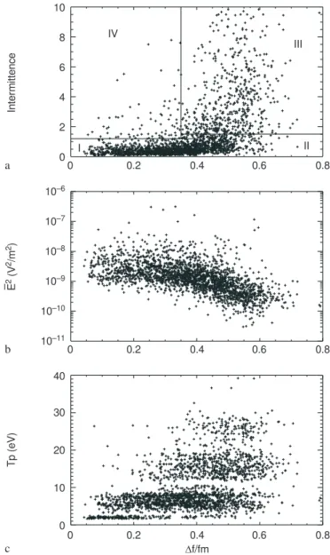
To illustrate how the spectral parameters and the intermittenceI (Eq. 4) allow us to separate the two types of low frequency waveforms, Fig. 2a displays a scatter plot ofI as a function ofDf=fm for all the TDS events
(2753) observed at fm<12 kHz. In this plane, four
regions have been delimited and two of them can be clearly identi®ed. Since IES are limited in time, they have a broad band Fourier spectrum and a large intermittence: Df=fm0:5 for the wave forms shown
in Fig. 1e, f while I '2 (Fig. 1e) and I '9 ( Fig. 1f). Thus IES are found in region III of Fig. 2a,
Df=fm>0:35 and I > 1.5. The LF wave packets are
more sinusoidal and correspond to region I,
Df=fm<0:4 andI 1.2; indeed they cover a narrower
frequency band and have a weaker intermittence. For example,Df=fm0:1 andI0:3 in Fig. 1b, the
corre-sponding values being 0:3 and 4 in Fig. 1c. Region II corresponds to wave forms which are not easily classi-®ed in one or the other category of wave forms, as for example the almost periodic succession of IES of Fig. 1d, for which Df=fm0:5 and I 0:6. Finally,
region IV corresponds to very short wave packets such as the one displayed in Fig. 1c.
Note that the Langmuir wave events have a very small relative band width and a small intermittence: for the wave form of Fig. 1a,Df=fm= 0.017 andI = 0.65.
Figure 2b displays the integrated energy density E2 (Eq. 3, in V2mÿ2) of the LF e.s. events as a function of
their relative band width Df=fm. The range is 310ÿ11
to 310ÿ7V2mÿ2 (the Langmuir waves, not shown,
have the same energy density range). E2, integrated
during the 17 ms of each event, decreases when Df=fm
increases: IES, which have the same amplitude as wave packets (Fig. 1), have a lower energy density because they are more intermittent (Fig. 2a).
It is also interesting to note that the proton temper-atureTp in the solar wind appears to be correlated with
the spectral properties of the LF wave activity. This is illustrated by Fig. 2c which displays a scatter plot in the plane [Df=fm,Tp] for the TDS events. A comparison of
Fig. 2b and c indicates that the events observed when Tp10 eV have a relatively broad band (Df=fm0:3)
and thus carry a weaker energy densityE2. We have not
found any correlation between the electron temperature and Df=fm or E2. In Sect. 6, we shall discuss in more
details the correlations between the wave properties and the solar wind parameters.
0 0.2 0.4 0.6 0.8
IV
III
II I
10
8
6
4
2
0
10–6
10–7
10–8
10–9
10–10
10–11
40
30
20
10
0
E(
V
/m
)
22
2
0 0.2 0.4 0.6 0.8
0 0.2 0.4 0.6 0.8
f/fm
Tp (
e
V)
b
c a
In
te
rm
itte
n
c
e
4 Properties of the low frequency wave packets
We shall now study the properties of the low frequency wave packets seen by the TDS and show that they have, besides their frequency range, all the properties of the IAC waves as described for example in the review by Gurnett (1991).
4.1 Polarisation
We ®rst note that, when the magnetic and electric wave forms were available, at the lowest sampling rate used here, no signi®cant magnetic counterpart was observed, indicating that in the range of frequency fpif fpe
the waves are basically electrostatic.
On the other hand, the TDS provides simultaneous measurements Ex and Ey of the electric ®eld amplitude
on the two orthogonal x and y antennas. These measurements may be used to obtain the polarisation of the waves and some information about the direction of the electric ®eld in the plane of the two antennas. Indeed, if DVx and DVy are the potential dierences
measured respectively at the terminals of the x and y-antenna, their ratio rxyDVy=DVx is a function of the
angle between the electric ®eld E and the unit vector along the x-antenna, ax. However, since the y-antenna
is much shorter than the x-antenna, the corresponding signal-to-noise ratio is much lower; so that in order to measure rxy the only reliable method is to perform a
linear regression DVy aDVxb and to assume that
the coecient a is a good estimate forrxy. The results
are shown in Fig. 3, which display a scatter plot of the antenna ratio rxy versus the cosine of the angle hxB
between ax and the magnetic ®eld B. In Fig. 3a, rxy is
shown for the wave packets and in Fig. 3b for the IES. It is clear thatrxy tends to decrease whenhxB decreases,
as expected if E is aligned with B. More precisely, let us calculate the ratio rxy obtained by assuming a
triangular distribution of current along the antennas and a monochromatic wave with a wave vector kLx1:1, typical of the wave packets, as we shall see
in Sect. 4.2. Let us also assume that the wave vector k
is aligned with B, so thathxkhxB. The expression for DVx is then
DVx/Lxcos hxB
sin kLxcoshxB=2
kLxcoshxB=2
2
5
and a similar expression forDVy. The theoretical ratiorxy
calculated in this way is the function of hxB shown in
Fig. 3a (solid line) forLy=Lx'0.1. It is equal to zero for hxB0 (the y-antenna is insensitive to electric ®elds
aligned with thex-antenna), it increases ashxBincreases
towards p=2, and it exhibits a divergence at hxB'p=2
(thex-antenna is insensitive to electric ®elds aligned with they-antenna). For small angles the theoretical curve is compatible with the data, indicating that the antennas behave as expected. However, the divergence of the rxy
data expected at large angles is not seen, a fact which may be explained in several ways. First, only TDS
events where the electric ®eld on thex-antenna is above a certain threshold are collected, so that very large values of rxy are not expected. Second, since we use
interpolated key parameter ®le magnetic ®eld data, our estimate of the angle hxB is probably not good enough,
especially close top=2. Furthermore, due to the presence of the spacecraft, the antennas may not behave exactly as orthogonal electric dipoles aligned with the physical antennas.
A similar trend is observed for the IES (see Fig. 3b), the ratio rxy also increasing with hxB. A theoretical
prediction ofrxy is however much harder to calculate for
IES without a model of the original (non sinusoidal) waveform in the plasma. Nevertheless, two conclusions may be drawn. First, the fact that the ratiorxy between
the output of the two antennas is correlated with the angle hxB between the local magnetic ®eld and the
x-antenna reinforces the argument of Sect. 3: the observed signals are not parasites (such as the shadow artefact described) but are produced in the solar wind plasma. Second, our results are consistent with the hypothesis that the wave vector is more or less aligned with the magnetic ®eld, for IES as well as for the LF wave packets. The use of magnetic ®eld data with a higher temporal resolution could help to be more speci®c.
0 0.2 0.4 0.6 0.8 1.0
0 0.2 0.4 0.6 0.8 1.0
cos XB 0.40
0.30
0.20
0.10
0 0.40
0.30
0.20
0.10
0
r=
V
/
V
XY
Y
X
r=
V
/
V
XY
Y
X
a
b
Fig. 3a, b. Scatter plot of the ratiorxyof the voltage dierencesDVy and DVx measured respectively on the y and xantenna versus the cosine of the anglehxBbetween the magnetic ®eld and the direction of thex-antennaafor wave packets; thesolid lineis a theoretical ratio
4.2 Doppler eect and wavelength
Let us now analyse of the Doppler eect on the observed frequencies. Consider ®rst the LF wave packets and let f0 be their frequency in the plasma rest frame, k their
wave vector (k2p=k being the corresponding wave-length) and f their frequency in the spacecraft frame. Since the waves are propagating along the local magnetic ®eld direction b, kkb, the relation between f0 and f can be written as .
f fpi
f0 fpi
kkD DfDopp
fpi
6
where
DfDopp
fpi
M
m
1=2
VswcoshBV
vthe
7
is the Doppler contribution to the observed frequency when kkD1, and hBV is the angle between the solar
wind velocity andb.
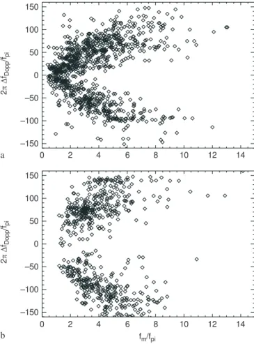
Figure 4a shows a scatter plot of the relative frequency fm=fpi versus 2pDfDopp=fpi for the LF wave
packets observed by the TDS, during the 19 days with the highest sampling rate, and selected as described in
Sect. 3 (region I of Fig. 2a). The cloud of points is V-shaped with a tip located around coshBV '0 and
fm=fpi1 and two linear branches, one for each sign
of coshBV. This result can be understood on the basis of
Eq. 6 if the main contribution to the observed frequen-cies comes from the Doppler eect, thus con®rming the previous analysis by Gurnett and Frank (1978). It is also consistent with the results obtained already that the waves are propagating along the ambient B ®eld. It shows further that the wave numbers of the wave packets do not cover a wide range. By estimating the slopes of the straight lines between which most of the points of Fig. 4a can be found, we ®nd
10 k
kD
50 or 0:1kkD0:6 : 8
Note that this estimate of the range of wave numbers of the LF wave packets is actually an upper limit, part of the scatter in Fig. 4a being probably due to the use of 1.5 min resolution magnetic and plasma data.
These results are compatible with the usual disper-sion relation of the ion acoustic waves; indeed, if we assume that the wave packets obey the linear, low frequency, dispersion relation
f0
fpi
kkD 1
3Tp
Te
1=2
9
we ®nd that the frequency in the plasma frame lies typically in the interval 0:1f0=fpi2 which is both
the range of values observed in Fig. 4a when the magnetic ®eld is nearly perpendicular to the solar wind velocity, and the typical range of ion acoustic waves. It has been suggested (Marsch, 1985) that waves observed in the rangefpi<f <fpe, in the Earth's foreshock, were
electron acoustic waves supported by the two electron populations (core and halo electrons). But the electron acoustic waves have a rest frame frequency higher than fpi, for parameters usually found in the solar wind, i.e.
higher thanf0 deduced from Fig. 4a.
We note in Fig. 4a that no wave packet has a frequency (in the spacecraft frame) lower than '0:3fpi
('200 Hz), and this minimum frequency is obtained when coshBV '0. Therefore the Doppler eect always
increases the frequency, independently of the sign of the radial component of the magnetic ®eld. This shows that the wave vector i.e. the direction of propagation of the observed wave packet, even if aligned withB, is oriented towards the Earth. It is unlikely that this result could be due to an observational bias. First, the total duration ('17 ms) of a TDS event at the highest sampling rate allows to resolve wave packets with frequencies of the order of 60 Hz. Second, the threshold above which an event is retained for an eventual transmission by the TDS experiment depends on the frequency, being about '50lV/m at a few kHz, and signi®cantly higher, '200lV/m, below 500 Hz, in order to reject more eciently low frequency aliases. However these instru-mental limitations cannot explain why a signi®cant number of wave packets with relative frequency fm=fpi0:3 were observed, and none below.
0 2 4 6 8 10 12 14
0 2 4 6 8 10 12 14
f /fm pi 150
100
50
0
–50
–100
–150
2f
/f
D
opp
pi
2f
/f
D
opp
pi
150
100
50
0
–50
–100
–150 a
b
To summarise this section, the waves measured by the TDS are electrostatic waves, with a wavelength of a few tens of Debye lengths propagating along the local magnetic ®eld. In the plasma frame they have a low frequency f0fpi, which is shifted upwards by the
Doppler eect into the range fpif <fpe in the
spacecraft frame. Therefore we have established ®rmly the relation between the LF wave forms observed by TDS and the electrostatic activity known as IAC waves. In conclusion, the observational evidence accumulated in the past and with the TDS experiment indicates that the IAC waves are coherent wave packets propagating along the ambient B ®eld, with wave numbers and frequencies compatible with the dispersion relation of ion acoustic waves.
5 Properties of the isolated electrostatic structures
IES similar to the ones shown in Fig. 1e, f are frequently observed; in many cases, the LF wave packets look like a rapid, nearly periodic succession of individual IES (Fig. 1d).
5.1 Doppler eect and spatial width
To estimate the spatial extension of the IES on a statistically signi®cant sample, we have used a method similar to the one used to analyse the Doppler eect on the LF wave packets. Indeed, for a non periodic signal which is limited in time, the mean frequency fm is
proportional to the inverse of the duration Dt of the signal, fm'1=Dt. This has been checked on a limited
sample of events which we have analysed in detail, with the expected result that the relation is true when the TDS event contains only one or very few spikes. Therefore, it is possible to use the spectral characteristics described in Sect. 3. The spatial extent along B of an IES, normalised to the local Debye length, can be estimated as
Dx
kD
'2pfpe
fm
VswcoshVB
vthe
10
if the IES velocity in the solar wind frame is negligible. We shall limit ourselves here to the events belonging to region III of Fig. 2a, i.e. with suciently large relative band width and intermittence, Df=fm> 0.35, I> 1.5:
this region only contains TDS events made of a small number of IES so as to minimise the aliasing produced by the presence of several IES in the same TDS event. For those IES, Fig. 4b shows the scatter plot of fm=fpi
versusDfDopp=fpi (Eq. 7). Once again we obtain a cloud
of points which is roughly V-shaped, showing that the main part of the observed temporal width of an IES is due to the advection by the solar wind of the structure past the spacecraft. This shape con®rms the inference that the IES are indeed propagating along the magnetic ®eld, as do the wave packets, with a speed which is small compared to the solar wind velocity.
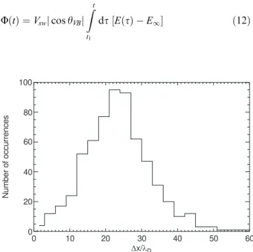
Figure 5 displays the corresponding histogram of spatial widths of the IES (Eq. 10), a typical value being '25kD. Once again it is hard to decide whether the
width of the histogram is real or results from the use of low resolution magnetic ®eld and plasma parameters.
5.2 Potential jump
Assuming that the IES are one-dimensional structures varying only along the magnetic ®eld, we can easily determine the spatial pro®les of the corresponding electric ®eld, electric potential U and charge density
dq. To obtain the sign of the electric ®eld we must take into account the orientation of the antenna ax with
respect to the solar wind velocity, measured by coshxV axVsw=Vsw.
Let us callEthe electric ®eld along the magnetic ®eld; it is related to the voltageDVxmeasured at thex-antenna
terminals by the relation
E t ÿDVxsign coshxV= LxjcoshxBj : 11
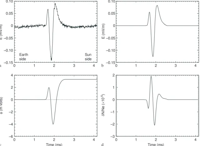
with the convention that it is positive if directed towards the Earth i.e. alongVsw. This electric ®eldE tis shown
in Fig. 6a for the largest IES of Fig. 1f. We have only considered here a ®nite time interval [t1;t2] of duration
'4:2 ms and containing'500 points around the time of maximum. This interval has been chosen so that it was possible to de®ne unambiguously two asymptotic states where the ®eld is almost constant and equal toE1which
has been taken as the zero of the electric ®eld. To eliminate the high frequency noise of Fig. 6a, the time pro®le has been smoothed over 10 points in the region of rapid variation and set to zero outside; the resulting electric ®eld pro®le is shown in Fig. 6b. The potentialU
is calculated from the de®nition as
U t VswjcoshVBj Zt
t1
dsE s ÿE1 12
0 10 20 30 40 50 60
x/ D 100
80
60
40
20
0
N
um
ber
of
occur
rences
while the charge separation dN NpÿNe is obtained
from Poisson's equation
dN t ÿ 1 4pqVswjcoshVBj
dE
dt : 13
The potential pro®le is shown in Fig. 6c. The remarkable feature is a ®nite potential jump of DU'3:3 mV between the two asymptotic states, the low potential side being towards the Earth. SinceDU is proportional to the average value hEi of the electric ®eld over the interval [t1;t2], the estimate of the potential jump is very
sensitive to the various osets which may aect the data and which we have supposed to be included in the non-zero value of E1. However it can be checked that, in
absolute value, hEi is signi®cantly higher than E1, so
that our estimate of the potential jump is not seriously aected.
We have repeated the calculation for a signi®cant number (75) of IES which have been chosen so that (1) they are clearly isolated structures (obtained by selecting TDS events of suciently high intermittenceI 5) and (2) the geometry is simple. By the latter we mean that the acute angles between the directions of the x-antenna, of
Band of the solar wind velocity are all smaller than 45.
The results were similar to those shown in Fig. 6. Figure 7 displays the histogram of the normalised potential jumps qDU= kBTemeasured for these 75 IES; a typical
value is qDU= kBTe '310ÿ4.
Therefore, the isolated electrostatic structures are actually weak double layers (WDL) with small relative amplitudes. They consist (see Fig. 6d) of two main layers of approximatively opposite charge, the positively charged one usually preceding the negatively charged one. Note that besides these two layers, one may distinguish a small negative precursor and a positive trailing region. The corresponding density ¯uctuation
dN=N is very small'10ÿ5. The similarity with the WDL
observed in the auroral regions (Mozer and Temerin,
0.10
0.05
0
–0.05
–0.10
–0.15
0.10
0.05
0
–0.05
–0.10
–0.15
E (
m
V/
m)
E (
m
V/
m)
4
2
0
–2
–4
–6
2
1
0
–1
–2
–3
(m
V
o
lts
)
N/
Ne
(
1
0
)
-5
Earth side
Sun side
a b
c d
0 1 2 3 4 0 1 2 3 4
0 1 2 3 4 0 1 2 3 4
Time (ms) Time (ms)
Fig. 6a±d. For the central double layer in Fig. 1f (between 8 and 9 ms), time pro®le of:athe measured electric ®eld (positive if directed towards the Earth);bthe electric ®eld smoothed over 10 points;cthe corresponding potential pro®le;dthe charge separationdNNpÿNe
–2 –1 0 1 2 3 4
qø/k T ( 10 )B e -3 0.50
0.40
0.30
0.20
0.10
0
P
robability of occurence
1983) is striking although there the peak amplitudes reach much higher values, qDU= kBTe '1. We have
also calculated the average electric ®eld and the poten-tial jump across short wave packets for which the asymptotic levels are clearly de®ned and, surprisingly, found a result not very dierent from the typical potential jumps across IES. For example, across the wave packet of Fig. 1c, the potential jump is qDU= kBTe 210ÿ4. For the 75 weak double layers
in the sample described, the potential jump (as a function of time) has generally the same sign as coshxV. Therefore, this potential usually drops towards
the Earth: it varies in the same sense as the interplan-etary electric potential which tends to decelerate the solar wind outward propagating electrons, or to accel-erate the protons. The weak double layers, as well as some wave packets, probably manifest a small scale charge separation due to a partial decoupling between electrons and protons on a Debye length scale. We have thus now to look for the solar wind regions where the electrostatic activity has been observed, and for the regions where the weak double layers are dominant.
6 Solar wind properties and electrostatic activity
We shall consider the question of how the electrostatic activity observed by the WIND/WAVES experiment depends on the local parameters of the solar wind. The 38-day period considered here is well suited for such an investigation since it exhibits a large range of variations of the physical properties of the solar wind. WIND was more then 85% of the time in the free solar wind i.e. not magnetically connected to the Earth's bow shock. It crossed three high speed ¯ows, two in the Northern magnetic ®eld Hemisphere, one in the Southern Hemi-sphere (Sandersonet al., 1998) and spent a long interval of time in a relatively low speed wind, in both hemispheres (Fig. 8). Six main crossings of the magnetic sector boundary were observed (days 142±143, 150, 158± 159, 165, 168±170 and 176) as well as four reverse interplanetary shocks (days 144, 150, 170 and 177). Unfortunately, however, natural electrostatic activity is observed by the TDS experiment only in regions of the solar wind where the particle density is below N 12 cmÿ3, because of the artefacts discussed in Sect. 2. As a
consequence, we were not able to make a complete statistical study of the occurrence of the IAC wave activity. Nevertheless, some interesting results have been obtained, which we shall now describe.
6.1 Synoptic view of the TDS observations
In Fig. 8, the electrostatic wave activity as observed by the TDS experiment is displayed as a function of time for two successive intervals of 19 days. Figure 8a covers the period from day 1995/05/20 (day 140) to 1995/06/07 (day 158), while Fig. 8b covers that from day 1995/06/08 (day 159) to 1995/06/26 (day 177). In the upper panels, the upper line gives the solar wind speed and the other
line the ratio Tp=Te. In the lower panels, the central
frequency and the band width (Eqs. 1 and 2) of every TDS event are indicated by a vertical bar centred onfm
with an extent of fm0:2Df. To illustrate the
limita-tions imposed on the TDS observalimita-tions, time intervals during which only artefacts are transmitted are indicated in Fig. 8a, b by bars at 30 Hz: this is the case, for example, on the days 159/95/06/08 and 169/95/06/18 (see Fig. 8b). The electron plasma frequency fpe12
kHz and gyrofrequency fce'100 Hz are given in each
®gure, as well as the Nyquist frequencies (3.8, 15 and 60 kHz) for the three sampling rates.
The e.s. activity occurs in two well-separated fre-quency bands, the LF band signi®cantly below the local electron plasma frequency fpe, and a narrow band
around fpe. In the high frequency range, our method
eliminates the waves at harmonics offpeexcept in a few
ambiguous cases. With these restrictions the Langmuir waves have a frequencyfmwhich follows very closely the
localfpe, con®rming the mode identi®cation. Sincefpe is
generally higher than 15 kHz, Langmuir waves can only be observed every two days, for the highest sampling rate. At the intermediate sampling rate (days 155 or 171 for example) aliasing of Langmuir waves are sometimes observed around 10 kHz.
Taking into account the limitations of the TDS observations, no apparent correlation can be found between the occurrence of the TDS activity and the plasma parameters displayed in Fig. 8, the solar wind speed and electron to proton temperature ratio: TDS events are observed on the day 151 (Vsw> 700 km/s,
Tp=Te>2) as well as on the day 164 (Vsw' 300 km/s,
Tp=Te<0.5).
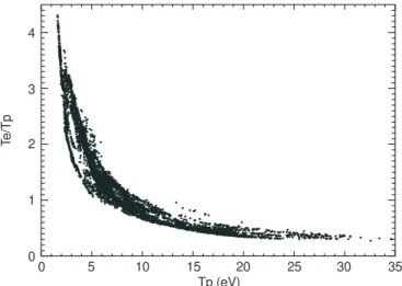
This is emphasised in Fig. 9: a 2D histogram of the values of [Vsw;Te=Tp] at all the times sampled by the TDS
is displayed as a one level contour line. The data ®ll a relatively narrow region of the plane, illustrating the well-known correlation between Vsw and Tp: fast winds
have higher proton temperatures than slow winds, the electron temperature having a smaller range of varia-tion. The energy density E2 of the 17 ms TDS events
(calculated using Eq. 3) is also shown as contours with grey levels in Fig. 9. It appears that the 17 ms TDS events have been observed for almost all solar wind conditions (except, of course, during periods of high density). The distribution of energy densityE2is almost
uniform in the [Vsw;Te=Tp] plane. There is however a
weak but signi®cant trend towards smaller energies in faster winds (with weaker Te=Tp). This trend is in
agreement with the Helios results (Fig. 5, 7 and 8 of Gurnettet al., 1979).
6.2 Correlation between the properties of the electrostatic waves and the solar wind parameters
weak double layers (region III of Fig. 2a) during the 19 days of the period studied here with the highest sampling rate.
We have found two parameters, namely the anglehBX
between the magnetic ®eld and the Earth-Sun direction
eX and the proton temperature Tp, which appear to
organise the data satisfactorily.
This is illustrated in Fig. 10a, b. Figure 10a displays the histogram of wave packets (dashed line), and WDL (solid line) in equal bins of jBX=Bj: the probability of
occurrence of wave packets does not depend on the modulus of coshBX, while the probability of WDL
events has a clear minimum for B perpendicular toeX,
and peaks for B along the Parker spiral and for more radial ®elds.
We have already shown (Sect. 3, Fig. 2b, c) that the events observed for Tp 10 or 11 eV have a relatively
broad band Df=fm 0.3 and a weaker energy density
E2. The scatter plot of Fig. 2c shows thatDf=f
mtends to
increase withTp. To illuminate the interpretation of the
scatter plot of Fig. 2c, Fig. 10b displays histograms ofTp
measured at the time of LF wave packets (dashed line) and of weak double layers (solid line). Crudely speaking, the wave packets and the WDL are both present when Tp<10 eV, while for higher proton temperatures Tp >
12 eV the WDL are dominant. Thus, the wave packets disappear gradually whenTpincreases from 10 to 30 eV.
Since there is a good correlation betweenTp andVswthis
disappearence of the wave packets is also observed for Vsw>500 km/s. This is probably the reason for the
Fig. 8a, b. Synopsis of the solar wind properties and e.s. activity: afrom May 20 to June 7, 1995. The numbers in abscissae indi-cate the beginning of the corre-sponding day of the year.Upper panel:Vsw andTp=Te.Lower
decrease of the electrostatic energy with increasing solar wind velocity mentioned in Sect. 6.1.
One would have expected that the temperature ratio Tp=Te, which is related to the damping of ion acoustic
waves, would also be correlated to the occurrence of wave packets. Indeed, the gradual disappearance of wave packets occurs forTp=Te1.2. However, a scatter
plot (not shown here) similar to Fig. 2c but for Tp=Te,
although exhibiting the same trend towards an increase of Df=fm with increasing Tp=Te, does so in a less
convincing way, just as one would expect if Te was a
statistically unrelated variable, with a range of variation 6 to 7 times smaller than that of Tp. There is thus no
evidence that a local macroscopic parameter like the temperature ratio Te=Tp plays a signi®cant role for the
type of the wave forms, contrary to theoretical
expec-tations and observations in other regions of the Earth environment (Kojima et al., 1994) and numerical sim-ulations (Omuraet al., 1994, 1996).
We conclude from Fig. 10 that isolated electrostatic structures, i.e. weak double layers, are found for any value ofTp but preferably when the ®eld is close to the
radial. The LF wave packets, i.e. TDS events with more sinusoidal wave forms are preferably found for low values ofTp, independently of the ®eld direction.
7 Discussion
It was totally unexpected to ®nd weak double layers in the free solar wind. These double layers are very weak, compared with those observed in numerical simulations (see Borovsky, 1984), in laboratory plasmas (see FaÈlt-hammar, 1993), or in the auroral regions (MaÈlkkiet al., 1993) where typically qD/'kBT. The whole LF e.s.
activity is only very weakly nonlinear, if the main source of nonlinearity is related to the macroscopic kinetic pressure, as is usually the case in the theoretical analysis of nonlinear ion acoustic waves (see e.g. Treumann and Baumjohann, 1997). Indeed, consider the equation of motion of the proton ¯uid:
@u
@t u ru ÿ q
Mr/ : 14
In the linear approximation, du being the velocity ¯uctuation andcs the sound speed, this gives
@du @t ' ÿcs
@du @x '
q M
@/
@x : 15
The degree of nonlinearity, i.e. the ratio between the nonlinear term in the left hand side of Eq. (14) and the electric restoring force, can be estimated as the Mach number du=cs'qDU=kBTe, which is generally weaker
than 10ÿ3 for LF wave packets as well as for WDL, as seen in Sect. 5.2. If we assume further that these ¯uctuations are weakly nonlinear ion acoustic waves with a typical wave vector k, their group velocity is of order vg 'cs1ÿ 3=2k2k2D. We can then de®ne a
typical time for the dispersal of a wave packet of width
Dx'2p=k via dispersive eects, sd 'Dx= csk2k2D and
compare it with the nonlinear time snl '1= kdu, the
ratio being
snl
sd
' kkD
2
2p
cs
du : 16
For the values of kkD'0.1 to 0.6 obtained in Sect. 4.2,
this ratio is typically of the order of 10 to 100, so that the dispersive eects are much stronger than the macro-scopic nonlinear eects. Since the wave forms shown in Fig. 1 are manifestly aected by nonlinear terms, this indicates that the corresponding source of nonlinearity is probably of microscopic origin.
The second result of our study is that the type of the e.s. waves depends on the proton temperature and on the direction of the magnetic ®eld. This result can be placed in a proper perspective if one recalls that the solar wind speed, density and proton temperature, and
200 300 400 500 600 700 800
Vsw (km/s) 4
3
2
1
0
Te
/T
p
Fig. 9 The thin line delimits the region of the plane [Vsw;Te=Tp] sampled by the TDS. Thegrey contoursgive the energy densityE2of the 17 ms TDS events, calculated with Eq. 3. The ®ve grey levels correspond to the valuesÿ12; ÿ10:5; ÿ9:35; ÿ8:75 andÿ7:75 for log10E2, in V2/m2
0 0.2 0.4 0.6 0.8 1.0 0 5 10 15 20 25 30 35
B /Bx Tp
0.25
0.20
0.15
0.10
0.05
0
0.3
0.2
0.1
0
P
robability of occurrence
a b
Fig. 10a, b. Histograms of the probability of occurrence of the IES (region III of Fig. 2a;solid line) and wave packets (region I of Fig. 2a,
the magnetic ®eld structure, are strongly dependent on the heliomagnetic latitude. Regions of high proton temperature and with more radial magnetic ®elds are likely to be found in the fast solar wind, at relatively high heliomagnetic latitudes. Away from the heliospher-ic current sheet, deep into the fast wind, LF wave packets are observed less and less frequently, and the e.s. activity occurs mainly in the form of WDL.
It is worthwhile mentioning that a number of proper-ties of the particle distribution functions depend also on the distance from the heliospheric current sheet, which explains why good correlations are usually found between IAC wave activity and non Maxwellian features of the distribution functions. For example, suprathermal elec-trons usually display an asymmetric structure in velocity space called astrahl(see Marsch, 1991, Sect. 8.2.3; Pilipp et al., 1987), a kind of beam more or less loosely aligned with the magnetic ®eld and directed towards the Earth. Pilippet al.(1987) noticed that the strahl disappears just at the magnetic sector boundary, and that the angular distribution of the strahl around the magnetic ®eld is narrower far from the heliospheric current sheet. It would be interesting to correlate the three states of e.s. activity (wave packets, weak double layers, no e.s. activity) to the three types of electron distributions observed by Pilipp et al.(1987) (broad strahl, narrow strahl, isotropic). This correlation will be studied in a future work.
We want to stress that while Tp appears to be an
important parameter for the properties of the LF waves, the electron temperature Te has no in¯uence on this
electrostatic activity, so thatTp=Teis less important than
Tp. Indeed, in our data set, the type of the wave forms
depends essentially onTp, as discussed in Sect. 3 and 6.2;
and waves are observed in the whole range 0.3 Te=Tp<4.5. What can be the in¯uence of the TDS data
selection on this result? We made a comparison (not shown here) of the histogram ofTp=Teat times when the
TDS transmitted a natural wave form, and of the corresponding histogram for all the 3D-Plasma points every 1.5 min during the considered 38 days: these histograms are very similar, with the same extrema Tp=Te0:2 and Tp=Te'3:5; the ®rst histogram peaks
around 0.8, while the second one peaks around 0.6. Therefore, we do not expect that our limitation to data with a relatively low density is signi®cant in this respect. Our results on the dominant role of Tp dier from the
results of Gurnettet al.(1979) who gave evidence for an in¯uence of Te=Tp. Actually, this contradiction is only
apparent since there is a strong anticorrelation between Te=Tp and Tp, partly due to the fact that the range of
variation of Te is much smaller than that of Tp. This
anticorrelation is displayed in Fig. 11, where the points correspond to all the TDS events, including artefacts, i.e. are typical of the solar wind at 1 UA.
8 Conclusion
The main results of the present analysis can be summarised as follows. When the density is smaller than about 10 cmÿ3, at the Lagrange point L
1, the time
domain sampler experiment detects a very bursty, but more or less continuous electrostatic activity in the frequency range between the ion and the electron plasma frequency, fpif <fpe. As seen with the TDS, this
electrostatic activity appears to be a mixture of coherent wave packets and weak double layers. A typical thickness of the double layers is 25kD; and a typical
value for the electric potential drop across the double layers is only a few mV, with qDU= kBTe '310ÿ4,
generally earthward. (When the solar wind density is larger than 10 cmÿ3an artefact prevents any observation
of the TDS activity.)
The highest intensity and level of wave activity in the range of frequency fpif <fpe is found for relatively
low proton temperatures, at low heliomagnetic latitudes. Towards higher latitudes, the frequency of occurrence of wave packets decreases, and one observes mainly weak double layers deep into the fast solar wind. No clear relation with important plasma parameters like the electron to proton temperature ratio was found.
To conclude, let us note that most of the Langmuir waves observed by the TDS are not associated with type III bursts and appear to be distributed as the low frequency activity described. Their detailed study will be the object of another investigation.
Acknowledgements. The WAVES instrument on WIND was built by teams at the University of Minnesota, the University of Iowa and the Observatoire de Paris, Meudon, with support of NASA/ GSFC. M. L. Kaiser is the Deputy PI. Use of the key parameter MFI data and 3D-plasma data is courtesy of the teams of the Magnetic Field Investigation experiment (PI R.P. Lepping) and the Three Dimensional Plasma experiment (PI R.P. Lin), and of the ISTP CDHF team at NASA/GSFC. The French contribution is supported by the Centre National d'Etudes Spatiales and the Centre National de la Recherche Scienti®que.
Topical Editor R. Schwenn thanks E. Marsch and another referee for their help in evaluating this paper.
References
Bale, S. D., D. Burgess, P. J. Kellogg, K. Goetz, R. L. Howard, and S. J. Monson, Phase coupling in Langmuir wave packets:
0 5 10 15 20 25 30 35
Tp (eV) 4
3
2
1
0
Te
/T
p
possible evidence of three-wave interactions in the upstream solar wind,Geophys. Res. Lett.,23,109±112, 1996.
Bale, S. D., D. Burgess, P. J. Kellogg, K. Goetz, and S. J. Monson, On the amplitude of intense Langmuir waves in the terrestrial electron foreshock,J. Geophys. Res.,102,11,281±286, 1997. Borovsky, J. E.,A review of plasma double-layer simulations, in
Second Symposium on Plasma Double Layers and Related Topics, Eds. R. Schrittwieser and G. Eder, Innsbruck, pp. 33± 54, 1984.
BostroÈm, R., G. Gustafsson, B. Holback, G. Holmgren, H. Koskinen, and P. Kintner, Characteristics of solitary waves and weak double layers in the magnetospheric plasma, Phys. Rev. Lett.,61,82, 1988.
Bougeret, J. -L., M. L. Kaiser, P. J. Kellogg, R. Manning, K. Goetz, S. J. Monson, N. Monge, L. Friel, C. A. Meetre, C. Perche, L. Sitruk, and S. Hoang, WAVES: the radio and plasma wave investigation on the WIND spacecraft,Space Sci. Rev,71,231± 263, 1995.
Dum, C. T., E. Marsch, W. G. Pilipp, and D. A. Gurnett,Ion sound turbulence in the solar wind, inSolar Wind Four, pp. 299±304, 1981.
FaÈlthammar, C. G.,Laboratory and space experiments as a key to the plasma universe, in Symposium on Plasma-93, Allahabad, India, 1993.
Forslund, D. W., Instabilities associated with heat conduction in the solar wind and their consequences,J. Geophys. Res.,75,17± 28, 1970.
Gary, S. P., Ion-acoustic-like instabilities in the solar wind,
J. Geophys. Res.,83,2504±2510, 1978.
Gary, S. P.,Theory of space plasma microinstabilities, Cambridge University press, 1993.
Gurnett, D. A., Waves and instabilities, in Physics of the inner heliosphere II, Eds. R. Schwenn and E. Marsch, Springer-Verlag, Berlin Heidelberg New York, pp. 135±157, 1991. Gurnett, D. A., and R. R. Anderson,Plasma wave electric ®elds in
the solar wind: initial results from Helios 1,J. Geophys. Res.,82, 632±650, 1977.
Gurnett, D. A., and L. A. Frank, Ion acoustic waves in the solar wind,J. Geophys. Res.,83,58±74, 1978.
Gurnett, D. A., E. Marsch, W. Pilipp, R. Schwenn, and H. Rosenbauer, Ion acoustic waves and related plasma observa-tions in the solar wind,J. Geophys. Res.,84,2029±2038, 1979. Kellogg, P. J., S. J. Monson, K. Goetz, R. L. Howard, J. -L. Bougeret, and M. L. Kaiser,Early Wind observations of bow shock and foreshock waves,Geophys. Res. Lett.,23,1243±1246, 1996.
Kojima, H., H. Matsumoto, T. Miyatake, I. Nagano, A. Fujita, L. A. Frank, T. Mukai, W. R. Paterson, Y. Saito, S. Machida, and R. R. Anderson, Relation between electrostatic solitary waves and hot plasma ¯ow in the plasma sheet boundary layer: GEOTAIL observations, Geophys. Res. Lett., 21, 2919±2922, 1994.
Kurth, W. S., D. A. Gurnett, and F. L. Scarf, High-resolution spectrograms of ion acoustic waves in the solar wind,
J. Geophys. Res.,84,3413±3419, 1979.
Lemons D. S., J. R. Asbridge, S. J. Bame, W. C. Feldman, S. P. Gary and J. T. Gosling,The source of electrostatic ¯uctuation in the solar wind,J. Geophys. Res.,84,2135, 1979.
Lepping, R. P., M. H. AcunÄa, L. F. Burlaga, W. M. Farrell, J. A. Slavin, K. H. Schatten, F. Mariani, N. F. Ness, F. M. Neubauer, Y. C. Whang, J. B. Byrnes, R. S. Kennon, P. V. Panetta, J. Scheifele, and E. M. Worley, The Wind magnetic ®eld investi-gation, in The global Geospace mission, Ed. C.T. Russell, Kluwer Academic Publishers, pp. 207±229, 1995.
Lin, N., P. J. Kellogg, R. J. MacDowall, A. Balogh, R. J. Forsyth, J. L. Phillips, A. Buttighoer, and M. Pick, Observations of
plasma waves in magnetic holes,Geophys. Res. Lett.,22, 3417± 3420, 1995a.
Lin, R. P., K. A. Anderson, S. Ashford, C. Carlson, D. Curtis, R. Ergun, D. Larson, J. McFadden, M. McCarthy, G. K. Parks, H. ReÁme, J. M. Bosqued, J. Coutelier, F. Cotin, C. d'Uston, K.-P. Wenzel, T. R. Sanderson, J. Henrion, J. C. Ronnet, and G. Paschmann,A three-dimensional plasma and energetic particle investigation for the Wind spacecraft, inThe global Geospace mission, Ed. C.T. Russell, Kluwer Academic Publishers, pp. 125±153, 1995b.
MacDowall, R. J., R. A. Hess, N. Lin, G. Thejappa, A. Balogh, and J. L. Phillips,Ulysses spacecraft observations of radio and plasma waves: 1991±1995,Astron. Astrophys.,316,396±405, 1996. MaÈlkki A., Eriksson A. I., Dovner P., R. BostroÈm, B. Holback, G.
Holmgren, and H. E. J. Hoskinen,A statistical study of auroral solitary waves and weak double layers, 1. Occurrence and net voltage,J. Geophys. Res.,98,15521, 1993.
Marsch, E.,Beam-driven electron acoustic waves upstream of the Earth's bow shock,J. Geophys. Res.,90,6327±6336, 1985. Marsch, E.,Kinetic physics of the solar wind plasma, inPhysics of
the inner heliosphere II, Eds. R. Schwenn and E. Marsch, Springer-Verlag, Berlin Heidelberg New York, pp. 45±133, 1991.
Matsumoto, H., H. Kojima, T. Miyatake, Y. Omura, M. Okada, I. Nagano, and M. Tsutsui,Electrostatic solitary waves (ESW) in the magnetotail: BEN wave forms observed by GEOTAIL,
Geophys. Res. Lett.,21,2915±2918, 1994.
Meetre, C., K. Goetz, R. Manning, J. -L. Bougeret, and C. Perche, A realtime neural network in space, Lund, July 29±31, 1997, in press in ESA Publications, 1998.
Meyer-Vernet, N., and C. Perche,Toolkit for antennae and thermal noise near the plasma frequency,J. Geophys. Res., 94,2405± 2415, 1989.
Mottez, F., S. Perraut, A. Roux, and P. Louarn, Coherent structures in the magnetotail triggered by counterstreaming electron beams,J. Geophys. Res.,102,11399±11408, 1997. Mozer, F. S., and M. Temerin,Solitary waves and double layers as
the source of parallel electric ®elds in the auroral acceleration region, in High Latitude Space Plasma Physics, Eds. B. Hultqvist and T. Hagfors, Plenum, London, 44, pp. 453, 1983. Omura, Y., H. Kojima, and H. Matsumoto,Computer simulation of electrostatic solitary waves: a nonlinear model of broadband electrostatic noise,Geophys. Res. Lett.,21,2923±2926, 1994. Omura, Y., H. Matsumoto, T. Miyake, and H. Kojima,Electron
beam instabilities as generation mechanism of electrostatic solitary waves in the magnetotail,J. Geophys. Res.,101,2685± 2697, 1996.
Pilipp, W. G., H. Miggenrieder, K. -H. Mulhauser, H. Rosenbauer, R. Schwenn, and F. M. Neubauer, Variations of electron distribution functions in the solar wind,J. Geophys. Res.,92, 1103±1118, 1987.
Richaume, P., J. -L. Bougeret, C. Perche, and S. Thiria,Simulation des traitements reÂseaux de neurones embarqueÂs sur la sonde spatiale Wind/Waves, inNeural networks and their applications 1994, pp. 141±150, 1995.
Sanderson, T. R., R. P. Lin, D. Larson, M. P. McCarthy, G. K. Parks, J. M. Bosqued, N. Lormant, K. Ogilvie, R. P. Lepping, A. Szabo, A. J. Lazarus, J. Steinberg, and J. T. Hoeksema,Wind observations of the in¯uence of the Sun's magnetic ®eld on the interplanetary medium at 1 AU,J. Geophys. Res.,103,17 235± 17 247, 1998.
Temerin, M., K. Cerny, W. Lotko, and F. S. Mozer,Observations of double layers and solitary waves in the auroral plasma,Phys. Rev. Lett.,48,1175±1179, 1982.
![Fig. 9 The thin line delimits the region of the plane [V sw ; T e =T p ] sampled by the TDS](https://thumb-eu.123doks.com/thumbv2/123dok_br/18399063.358466/12.892.65.431.91.350/fig-line-delimits-region-plane-v-sampled-tds.webp)