Antônio F. B. Almeida Prado
Member, ABCM
[email protected] Instituto Nacional de Pesquisas Espaciais - INPE Caixa Postal 515 12227-010 São José dos Campos, SP, Brazil
Orbital Maneuvers Between the
Lagrangian Points and the Primaries
in the Earth-Sun System
This paper is concerned with trajectories to transfer a spacecraft between the Lagrangian points of the Sun-Earth system and the primaries. The Lagrangian points have important applications in astronautics, since they are equilibrium points of the equation of motion and very good candidates to locate a satellite or a space station. The planar circular restricted three-body problem in two dimensions is used as the model for the Sun-Earth system, and Lamaître regularization is used to avoid singularities during the numerical integration required to solve the Lambert's three-body problem. The results show families of transfer orbits, parameterized by the transfer time.
Keywords: Astrodynamics, lagrangian points, orbital maneuvers, impulsive transfers
Introduction
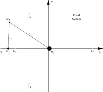
The well-known Lagrangian points that appear in the planar restricted three-body problem (Szebehely, 1967) are very important for astronautical applications. They are five points of equilibrium in the equations of motion, what means that a particle located at one of those points with zero velocity will remain there indefinitely. Their locations are shown in Fig. 1. The collinear points (L1, L2 and L3) are always unstable and the triangular points (L4 and L5) are stable in the present case studied (Sun-Earth system). They are all very good points to locate a space-station, since they require a small amount of ∆V (and fuel) for station-keeping. The triangular points are specially good for this purpose, since they are stable equilibrium points.1
In this paper, the planar restricted three-body problem is regularized (using Lamaître regularization) and combined with numerical integration and gradient methods to solve the two point boundary value problem (the Lambert's three-body problem). This combination is applied to the search of families of transfer orbits between the Lagrangian points and the primaries, in the Sun-Earth system, with the minimum possible energy. This paper is a continuation of two previous papers that studied transfers in the Earth-Moon system: Broucke (1979), that studied transfer orbits between the Lagrangian points and the Moon and Prado (1996), that studied transfer orbits between the Lagrangian points and the Earth.
The Planar Circular Restricted Three-Body Problem
The model used in all phases of this paper is the well-known planar circular restricted three-body problem. This model assumes that two main bodies (M1 and M2) are orbiting their common center of mass in circular Keplerian orbits and a third body (M3), with negligible mass, is orbiting these two primaries. The motion of M3 is supposed to stay in the plane of the motion of M1 and M2 and it is affected by both primaries, but it does not affect their motion (Szebehely, 1967). The canonical system of units is used, and it implies that: i) The unit of distance (l) is the distance between M1 and M2; ii) The angular velocity (ω) of the motion of M1 and M2 is assumed to be one; iii) The mass of the smaller primary (M2) is
given by µ =
2 1
2
m m
m
+ (where m1 and m2 are the real masses of M1
Paper accepted October, 2005. Technical Editor: Atila P. Silva Freire.
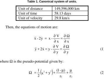
and M2, respectively) and the mass of M2 is (1-µ), so the total mass of the system is one; iv) The unit of time is defined such that the period of the motion of the primaries is 2π; v) The gravitational constant is one. Table 1 shows the values for these parameters for the Sun(M1)-Earth(M2) system, that is the case considered in this paper.
Table 1. Canonical system of units.
Unit of distance 149,596,000 km Unit of time 58.13 days Unit of velocity 29.8 km/s
Then, the equations of motion are:
x = x V -x = y 2 -x
∂ Ω ∂ ∂ ∂
y = y V -y = x 2 + y
∂ Ω ∂ ∂ ∂
(1)
where Ω is the pseudo-potential given by:
(
)
r + r
) -1 ( + y + x 2 1 =
2 1 2 2
µ µ
Ω (2)
This system of equations has no analytical solutions, and numerical integration is required to solve the problem. This system has an invariant called Jacobi integral. There are many ways to define the Jacobi integral (see Szebehely, 1967, pg. 449). In this paper the definition shown in Broucke (1979) is used. Under this version, the Jacobi integral is given by:
(
x +y)
-( )
x,y =Const 21 =
E 2 2 Ω
(3)
The three-body problem has also two important properties: 1) The existence of five equilibrium points (called the Lagrangian points L1, L2, L3, L4 and L5, as seen in Fig. 1), that are
the points where x ∂
Ω ∂
= y ∂
Ω ∂
= 0. It corresponds to say that a
stable for µ < 0.03852, what means that they are stable in the present case (Sun-Earth), since µ = 0.0000030359. Their locations and potential energy are shown in Table 2.
X L3 M1
L L2 M2 1
Y L 5 L4 Fixed System M3 r r 2 1
Figure 1. Geometry of the problem of three bodies.
Table 2. Position and potential energy of the five Lagrangian points.
x y E0
L1 -0.9899909 0 -1.5004485
L2 -1.0100702 0 -1.5001481
L3 1.0000013 0 -1.5000015
L4 -0.4999969 +0.8660254 -1.4999984 L5 -0.4999969 -0.8660254 -1.4999984
2) The curves of zero velocity, that are curves given by the expression:
( )
x,y -=E0 Ω (3)
that is the equivalent of equation (2) in the special case where 0
= y =
x . They are important, because they determine forbidden and allowed regions of motion for M3 based in its initial conditions. More details about these and other properties of the three-body problem can be found in Szebehely (1967) and Broucke (1979).
Lamaître Regularization
The equations of motion given by Eqs. (1) are not suitable for numerical integration in trajectories passing near one of the primaries. The reason is that the positions of both primaries are singularities in the potential V (since r1 or r2 goes to zero, or near zero) and the accuracy of the numerical integration is affected every time this situation occurs. The solution for this problem is the use of regularization, that consists in a substitution of the variables for position (x-y) and time (t) by another set of variables (ω1, ω2, τ),
such that the singularities are eliminated in these new variables. Several transformations with this goal are available in the literature (Szebehely, 1967, chapter 3), like Thiele-Burrau, Lamaître and Birkhoff. They are called "global regularization", to emphasize that both singularities are eliminated at the same time. The case where
only one singularity is eliminated at a time is called "local regularization". For the present research the Lamaître's regularization is used. To perform the transformation it is necessary first to define a new complex variable q = q1 + iq2 (i is the imaginary unit), with q1 and q2 given by:
y q , 2 / 1 x
q1= + −µ 2= (4)
Now, in terms of q, the transformation involved in Lamaître regularization is given by:
ω ω
ω 2 12
+ 4 1 = ) ( f = q (5)
for the old variables for position (x-y) and:
( )
ω ω ω τ ∂ ∂ 6 4 2 2 4 = ' f =t -1
(6)
where f '(ω) denotes ω ∂ ∂f
, for the time.
In the new variables the equation of motion of the system is:
* 2 grad = ' ) ( ' f '+2i
' ω ω Ω
ω ω (5)
where ω = ω1 + iω2 is the new complex variable for positions, ω' and ω" denotes first and second derivatives of ω with respect to the
regularized time τ, gradωΩ* represents
1 * ω ∂ Ω ∂
+ i
2 * ω ∂ Ω ∂
and Ω* is
the transformed pseudo-potential given by:
( )
ωΩ
Ω f' 2
*
2 C
-= (6)
where C = µ(1-µ) - 2E.
Equations (5) in complex variables can be separated in two second order equations in the real variables ω1 and ω2 and organized in the standard first order form, that is more suitable for numerical integration. The final form, after defining the regularized velocity components ω3 and ω4 as
ω
1' =
ω
3 andω
2' =
ω
4, is:3 ' 1=ω
ω
4 ' 2=ω
ω
( )
1 * 2 4 '3 2 f' ∂ω
Ω ∂ + ω ω = ω
( )
2 * 2 3 '4 2 f' ∂ω
Ω ∂ + ω ω − = ω (7)
Another necessary set of equations is the one to map velocity components from one set of variables to another. They are:
( )
( )
2 3 1 ' f ' f q ω ω ω =( )
The Mirror Image Theorem
The mirror image theorem (Miele, 1960) is an important and helpful property of the planar circular restricted three-body problem. It says that: "In the rotating coordinate system, for each trajectory defined by x(t),y(t),x(t),y(t) that is found, there is a symmetric (in relation to the "x" axis) trajectory defined by
(-t) y -(-t), x -y(-t),
-x(-t), ". The proof is omitted in this paper, but the reader can verify its veracity by substituting those two solutions in the equations of motion. With this property, there is no need to calculate the returning trajectories from the primaries to the Lagrangian points. For the collinear points, the symmetric of the trajectory that goes from the Lagrangian point to the Earth is the trajectory that goes from the Earth to the Lagrangian point. For the triangular points the situation is a little more complex, since these points are not in the "x" axis. The symmetric of the trajectory that goes from L4 to the Earth is the trajectory that goes from the Earth to L5 and the symmetric of the trajectory that goes from L5 to the Earth is the trajectory that goes from the Earth to L4.
The Lambert's Three-Body Problem
The problem that is considered in the present paper is the problem of finding trajectories to travel between the Lagrangian points and the primaries. Since the rotating coordinate system is used and all the primaries and the Lagrangian points are in fixed known positions, this problem can be formulated as:
"Find an orbit (in the three-body problem context) that makes a spacecraft to leave a given point A and goes to another given point B". That is the famous TPBVP (two point boundary value problem). There are many orbits that satisfy this requirement, and the way used in this paper to find families of solutions is to specify a time of flight for the transfer. Then, the problem becomes the Lambert's three-body problem, that can be formulated as:
"Find an orbit (in the three-body problem context) that makes a spacecraft to leave a given point A and goes to another given point B, arriving there after a specified time of flight". Then, by varying the specified time of flight it is possible to find a whole family of transfer orbits and study them in terms of the ∆V required, energy, initial flight path angle, etc.
The Solution of the TPBVP
The restricted three-body problem is a problem with no analytical solutions, so numerical integration is the only possible approach to solve it. To solve the TPBVP in the regularized variables the following steps are used:
i) Guess a initial velocity
V
i, so together with the initial prescribed positionr
i the complete initial state is known;ii) Guess a final regularized time τf and integrate the regularized equations of motion from τ0 = 0 until τf;
iii) Check the final position
r
f obtained from the numerical integration with the prescribed final position and the final real time with the specified time of flight. If there is an agreement (difference less than a specified error allowed) the solution is found and the process can stop here. If there is no agreement, an increment in the initial guessed velocity Vi and in the guessed final regularized time is made and the process goes back to step i).The method used to find the increment in the guessed variables is the standard gradient method, as described in reference 7. The routines available in this reference are also used in this research with minor modifications.
Numerical Results
The Lambert's three-body problem between the primaries and the Lagrangian points is solved for several values of the time of flight. Since the regularized system is used to solve this problem, there is no need to specify the final position of M3 as lying in an primary's parking orbit (to avoid the singularity). Then, to make a comparison with previous papers (Broucke, 1979 and Prado, 1996) the primary's center is used as the final position for M3. The results are organized in plots of the energy (as given by Eq. 3) and the initial flight path angle in the rotating frame against the time of flight. The definition of the angle is such that the zero is in the "x" axis, (pointing to the positive direction) and it increases in the counter-clock-wise sense. Plots of the trajectory in the rotating system are also included. This problem, as well as the Lambert’s original version, has two solutions for a given transfer time: one in the counter-clock-wise direction and one in the clock-wise direction in the inertial frame. In this paper, emphasis is given in finding the families with the smallest possible energy (and velocity at the Lagrangian points, as a consequence of Eq. 3), although many other families do exist.
Trajectories from L1
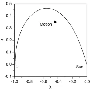
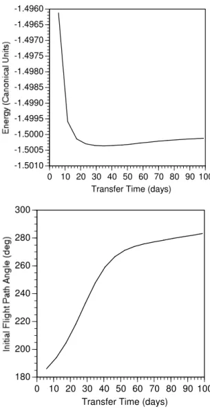
In the nomenclature used in this paper, L1 is the collinear Lagrangian point that exists between the Sun and the Earth. It is located about 1,496,867 km from the Earth. Figure 2 shows the results for the least expensive family of transfers to the Sun that was found in this research and Fig. 3 shows the transfers to the Earth. The local minimum for a transfer to the Sun occurs for a time of flight close to 64 days, requires an energy E = -1.0101 and has a initial flight path angle of 90 deg. In terms of velocity increment (∆V) it means an impulse of 29.5 km/s (0.9903 canonical units) applied at L1. For a transfer to the Earth, the minimum occurs for a time of flight close to 35 days, requires an energy E = -1.5004 and has a initial flight path angle of 248 deg. In terms of velocity increment (∆V) it means an impulse of 0.298 km/s (0.01 canonical units) applied at L1.
-0.1 0.0 0.1 0.2 0.3 0.4 0.5
-1.0 -0.8 -0.6 -0.4 -0.2 0.0 Y
X
Sun L1
Motion
-1.20 -1.00 -0.80 -0.60 -0.40 -0.20 0.00
0 20 40 60 80 100 120 140 160 Transfer Time (days)
0 20 40 60 80 100 120 140
0 20 40 60 80 100 120 140 160 Transfer Time (days)
Figure 2. (Continued).
-0.006 -0.005 -0.004 -0.003 -0.002 -0.001 0.000 0.001
-1.000 -0.998 -0.996 -0.994 -0.992 -0.990 Y
X Earth
L1
Motion
Figure 3. Transfers from L1 to the Earth.
-1.5010 -1.5005 -1.5000 -1.4995 -1.4990 -1.4985 -1.4980 -1.4975 -1.4970 -1.4965 -1.4960
0 10 20 30 40 50 60 70 80 90 100 Transfer Time (days)
180 200 220 240 260 280 300
0 10 20 30 40 50 60 70 80 90 100 Transfer Time (days)
Figure 3. (Continued).
Trajectories from L2
-0.1 0.0 0.1 0.2 0.3 0.4 0.5
-1.2 -1.0 -0.8 -0.6 -0.4 -0.2 0.0 Y
X
L2 Sun
Motion
-1.00 -0.80 -0.60 -0.40 -0.20 0.00
0 20 40 60 80 100 120 140
Transfer Time (days)
0 20 40 60 80 100 120 140
0 20 40 60 80 100 120 140
Transfer Time (days)
Figure 4. Transfers from L2 to the Sun.
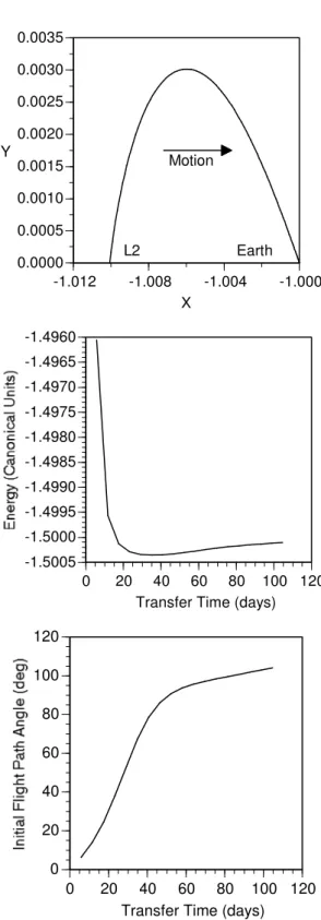
0.0000 0.0005 0.0010 0.0015 0.0020 0.0025 0.0030 0.0035
-1.012 -1.008 -1.004 -1.000 Y
X
Earth L2
Motion
-1.5005 -1.5000 -1.4995 -1.4990 -1.4985 -1.4980 -1.4975 -1.4970 -1.4965 -1.4960
0 20 40 60 80 100 120
Transfer Time (days)
0 20 40 60 80 100 120
0 20 40 60 80 100 120
Transfer Time (days)
Figure 5. Transfers from L2 to the Earth.
Trajectories from L3
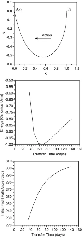
the Earth. The local minimum for a transfer to the Sun occurs for a time of flight close to 70 days, requires an energy E = -0.9965 and has a initial flight path angle of 275 deg. In terms of velocity increment (∆V) it means an impulse of 29.9 km/s (1.0035 canonical units) applied at L1. For a transfer to the Earth, the minimum occurs for a time of flight close to 169 days, requires an energy E = -1.4390 and has a initial flight path angle of 253 deg. In terms of velocity increment (∆V) it means an impulse of 10.4 km/s (0.3493 canonical units) applied at L1.
-0.6 -0.5 -0.4 -0.3 -0.2 -0.1 0.0 0.1
0.0 0.2 0.4 0.6 0.8 1.0 1.2
Y
X
L3 Sun
Motion
-1.00 -0.95 -0.90 -0.85 -0.80 -0.75 -0.70 -0.65 -0.60 -0.55 -0.50
0 20 40 60 80 100 120 140 160 Transfer Time (days)
220 230 240 250 260 270 280 290 300 310
0 20 40 60 80 100 120 140 160 Transfer Time (days)
Figure 6. Transfers from L3 to the Sun.
-0.2 -0.1 0.0 0.1 0.2 0.3
-1.0 -0.6 -0.2 0.2 0.6 1.0 Y
X Motion
Earth L3
-1.44 -1.43 -1.42 -1.41 -1.40 -1.39 -1.38 -1.37 -1.36
120 130 140 150 160 170 180 190 Transfer Time (days)
210 220 230 240 250 260 270
120 130 140 150 160 170 180 190 Transfer Time (days)
Figure 7. Transfers from L3 to the Earth.
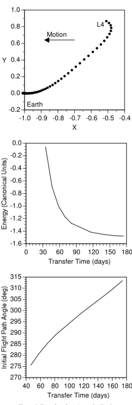
Trajectories from L4
minimum for a transfer to the Sun occurs for a time of flight close to 64 days, requires an energy E = -0.9999 and has a initial flight path angle of 29 deg. In terms of velocity increment (∆V) it means an impulse of 29.8 km/s (1.0001 canonical units) applied at L1. For a transfer to the Earth, the minimum occurs for a time of flight close to 174 days, requires an energy E = -1.4790 and has a initial flight path angle of 313 deg. In terms of velocity increment (∆V) it means an impulse of 6.1 km/s (0.2049 canonical units) applied at L1.
••••
•
•
•
•
•
•
•
•
•
•
•
•
•
•
•
•
•
••
•
•
•
•
•
•
•
•
•
•
•
••
•
•
•
•
•
••
•
•
•
•
•
••
•
•
•
••
•
••
•
•••
•
•••
•
•
•
•
•
•
•
•
•
•
•
•
•
•
•
•
•
•
•
•
•
•
•
•
•
•
•
•
•
•
•
•
•
•
•
0.0 0.1 0.2 0.3 0.4 0.5 0.6 0.7 0.8 0.9 1.0-0.5 -0.4 -0.3 -0.2 -0.1 0.0 0.1 0.2 Y X Motion Sun L4 -1.00 -0.95 -0.90 -0.85 -0.80 -0.75 -0.70
0 20 40 60 80 100 120 140 160 180 Transfer Time (days)
-10 0 10 20 30 40 50 60 70
0 20 40 60 80 100 120 140 160 180 Transfer Time (days)
Figure 8. Transfers from L4 to the Sun.
••••
•
•
•
•
•
•
•
•
•
•
•
•
•
•
•
•
•
•
•
•
•
•
•
•
•
•
••
••
••
••
•••
••••
••••••••
••••••••••••••••••••••••••••••••••••••••••••••••
-0.2 0.0 0.2 0.4 0.6 0.8 1.0-1.0 -0.9 -0.8 -0.7 -0.6 -0.5 -0.4 Y X Earth L4 Motion -1.6 -1.4 -1.2 -1.0 -0.8 -0.6 -0.4 -0.2 0.0
0 30 60 90 120 150 180
Transfer Time (days)
270 275 280 285 290 295 300 305 310 315
40 60 80 100 120 140 160 180 Transfer Time (days)
Figure 9. Transfers from L4 to the Earth.
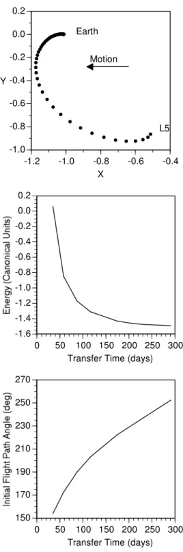
Trajectories from L5
a time of flight close to 64 days, requires an energy E = -0.9999 and has a initial flight path angle of 149 deg. In terms of velocity increment (∆V) it means an impulse of 29.8 km/s (1.0001 canonical units) applied at L1. For a transfer to the Earth, the minimum occurs for a time of flight close to 291 days, requires an energy E = -1.4910 and has a initial flight path angle of 252.40 deg. In terms of velocity increment (∆V) it means an impulse of 4.0 km/s (0.1342 canonical units) applied at L1.
•••
••
•
•
•
•
•
•
•
•
•
•
•
•
•
•
•
•
•
•
•
•
•
•
•
•
•
•
•
•
•
•
•
•
•
•
•
•
•
•
•
•
•
•
•
•
•
•
•
•
•
•
•
•
•
••
•
•
•
•
•
•
•
•
•
•
•
•
•
•
•
••
•
•
•
•
•
•
•
•
•
•
•
•
•
•
•
•
•
•
•
•••••
-1.0 -0.8 -0.6 -0.4 -0.2 0.0 0.2-0.8 -0.6 -0.4 -0.2 0.0 0.2 Y X Sun L5 Motion -1.1 -0.9 -0.7 -0.5 -0.3 -0.1 0.1
0 10 20 30 40 50 60 70 80 90 100 Transfer Time (days)
80 90 100 110 120 130 140 150 160 170 180
0 10 20 30 40 50 60 70 80 90 100 Transfer Time (days)
Figure 10. Transfers from L5 to the Sun.
•
•
•
•
•
•
•
•
•
•
•••••••••••••••••••••••••••••••••••••••••••••
•••••••
•
••••••
••••
•••
••
•
•••
••
•
•
•••
•
•••
•
••
•
•
•
••
-1.0 -0.8 -0.6 -0.4 -0.2 0.0 0.2-1.2 -1.0 -0.8 -0.6 -0.4 Y X Earth L5 Motion -1.6 -1.4 -1.2 -1.0 -0.8 -0.6 -0.4 -0.2 0.0 0.2
0 50 100 150 200 250 300 Transfer Time (days)
150 170 190 210 230 250 270
0 50 100 150 200 250 300 Transfer Time (days)
Figure 11. Transfers from L5 to the Earth.
Comparison with Transfers in the Earth-Moon
(fixed) system. In the sideral system, all bodies and points are rotating with unit angular velocity and it means that their linear velocity is equal to their distance from the center of the system. The Earth and the Lagrangian points have distances from the center of the system in the same order of magnitude (the approximate values are: Earth = 0.9999969, L1 = 0.9899909, L2 = 1.0100702, L3 = 1.0000013, L4 = L5 = 0.9999984), so their linear velocities are similar and a small ∆V is enough to cause an approximation and the rendezvous desired.
However, the Sun has a very small distance from the center (0.0000030359), and in consequence a very small linear velocity. As seen from the Sun, in the fixed coordinate system, to transfer a satellite from one of the Lagrangian points (or the Earth) to the Sun is equivalent to transfer a satellite from a high (about 1,500,000 km) circular orbit with a transverse velocity near 29.8 km/s (the circular velocity for this altitude) to the Sun. The best way to do it is to apply a ∆V of about 29.8 km/s in the opposite direction of the motion to reduce the velocity to a value in the order of magnitude of the velocity required by a Hohmann-type transfer (not the same value, because this is not a two-body problem, since the Moon is still acting in the system). The order of magnitude of this velocity is near zero, considering a two body Hohmann type transfer from the Lagrangian point to the center of the Earth. This means that a ∆V in the order of magnitude of 29.8 km/s is always required for those transfers, and there is no hope to reduce it by a large amount.
Conclusions
In this paper, the Lamaître regularization is applied to the planar restricted three-body problem to solve the Lambert's three-body problem (TPBVP) and it gives families of transfer orbits between
the primaries and all the five Lagrangian points that exist in the Sun-Earth system.
Families of transfer orbits with small residual velocities at the Lagrangian points were not found in this case, although they do exist in the case of transfers to the Moon. In particular, it means that the transfer with the absolute minimum ∆V between the Earth and the Moon passing by L1 was not found.
Acknowledgments
This work was funded by FAPESP (São Paulo State Foundation Research Fund) under the Grant 2000/14769-4 and CNPq (National Council for Scientific and Technological Development) under the Grant 1995/9290-1.
References
Broucke, R. 1979, “Traveling Between the Lagrange Points and the Moon”, Journal of Guidance and Control, Vol. 2, nº 4, July-Aug. pp. 257-263.
Farquhar, R. W. 1969, “Future Missions for Libration-point Satellites”, Astronautics and Aeronautics, May.
Miele, A. 1960, “Theorem of Image Trajectories in the Earth-Moon Space”, 11th International Astronautical Congress, Stockholm, Sweden, Aug. Astronautica Acta, pp. 225-232.
Prado, A.F.B.A. 1969, “Traveling Between the Lagrangian Points and the Earth”. Acta Astronautica, Vol. 39, no. 7, October, pp. 483-486.
Press, W. H.; Flannery, B. P.; Teukolsky, S. A. and Vetterling, W. T. 1989, “Numerical Recipes”, Cambridge University Press, NewYork.