M. P. de Abreu
Departamento de Modelagem Computacional Instituto Politécnico Universidade do Estado do Rio de Janeiro Caixa Postal 97282 28601-970 Nova Friburgo, RJ. Brazil [email protected]
A Mathematical Method for Solving
Mixed Problems in Multislab Radiative
Transfer
In this article, we describe a mathematical method for solving both conservative and non-conservative radiative heat transfer problems defined on a multislab domain, which is irradiated from one side with a beam of radiation. We assume here that the incident beam may have a monodirectional (singular) component and a continuously distributed (regular) component in angle. The key to the method is a Chandrasekhar decomposition of the (mathematical) multislab problem into an uncollided transport problem with singular boundary conditions and a diffusive transport problem with regular boundary conditions. Solution to the uncollided problem is straightforward, but solution to the diffusive problem is not so. For then we make use of a recently developed discrete ordinates method to get an angularly continuous approximation to the solution of the diffusive problem. We suitably compose uncollided and diffuse solutions, and the task of generating an approximate solution to the original multislab radiative transfer problem is complete. We illustrate the accuracy of the proposed method with numerical results for a test problem in shortwave atmospheric radiation, and we conclude this article with a discussion.
Keywords: Radiative transfer, multislab problems, mixed beams, conservative scattering, discrete ordinates
Introduction
We have been long working on the development of analytical and numerical methods for solving basic and important problems in neutron transport theory. These methods are intended to yield accurate solutions to discrete ordinates (SN) versions of the integrodifferential neutron transport equation (Davison, 1957; Duderstadt and Martin, 1979; Lewis and Miller Jr., 1993). Roughly speaking, an SN version of a transport equation consists of taking the integrodifferential transport equation in a finite set of angular directions (discrete ordinates), and replacing therewith the integral source term by a suitable quadrature formula. As a result, we obtain a coupled system of linear differential equations of the first order whose unknowns are approximations to the angular density of neutrons in the discrete directions considered. This system of linear differential equations is referred to as the SN equations (Lewis and Miller Jr., 1993). Discrete ordinates approximations to the boundary conditions can be likewise derived, and an SN problem is said to be stated (SN equations plus SN boundary conditions).1
The neutron transport problems that can be solved with our current SN methods can be divided into two major classes: multiplying and non-multiplying problems. The first class incorporates neutron transport problems defined in critical systems with respect to neutron fission chain reactions (de Abreu, Alves Filho and Barros, 1993, 1996; de Abreu and Barros, 1994; de Abreu, 1995, 1997). A typical problem in this class is that of computing thermal power distribution and neutron multiplication factor in nuclear reactor design and analysis (Duderstadt and Hamilton, 1976). The second class addresses those problems where neutron regeneration is only due to scattering events, and the boundary conditions are modelled by smooth functions of the angular variable (Barros and Larsen, 1990, 1991; de Abreu et al., 1998; de Abreu, 1998, 2001a, 2001b, 2002). A classical problem here is that of computing the emerging space-energy-angle distribution of neutrons due to a highly active neutron source in radiation shielding design (Shultis and Faw, 1996).
As noticed by S. Chandrasekhar (1950) more than a half century ago, the mathematical problems that arise in neutron transport
Paper accepted July, 2005. Technical Editor: Atila P. Silva Freire.
theory and radiative heat transfer are essentially the same. For example, some problems in the second class above and some problems in radiative transfer in planetary atmospheres (Chandrasekhar, 1950; Liou, 2002) and in vegetation canopies (Myneni and Ross, 1991; Ganapol et al., 1998, 1999) are formulated by essentially the same transport equation, with the differences lying only in the integral source terms. These matters have recently attracted our attention to the point that we have been dedicating part of our work with transport methods to the extension of some of our slab-geometry SN analytical and numerical methods to solve basic and important problems in the theory of radiative transfer. Unfortunately, things are not so straightforward. For example, the boundary conditions for radiative transfer problems are often more complicated than those in neutron transport due to the presence of interacting (absorbing-emitting-scattering) boundaries (Stamnes et al., 1988; Myneni and Ross, 1991; Liou, 2002). Also, basic and important problems in radiative transfer are characterized by highly anisotropic scattering (Garcia and Siewert, 1985; Liou, 2002). In this case, the phase function of the scattering angle is often approximated by a high order polynomial expansion. And, particularly in atmospheric radiative transfer, we have most often to solve conservative problems, i.e., those associated to the
conservative case of perfect scattering of radiation (Chandrasekhar,
solved basic and important problems in atmospheric radiative transfer such as the four azimuthally symmetric test problems posed in 1977 by the Radiation Commission of the International Association of Meteorology and Atmospheric Physics (Lenoble, 1985), as well as some multislab problems adapted from a six-layer model atmosphere discussed in a work of Devaux et al. (1979) on the facile (FN) method.
We find it appropriate at this point to make things clear as to what we mean when we speak of a multislab conservative problem and of a multislab non-conservative problem in radiative transfer. A standing point in the theory of radiative transfer is the formulation (and subsequent analysis) of conservative and non-conservative
problems defined in a homogeneous plane-parallel medium. These nomenclatures are direct reference to the conservative case of perfect scattering of a pencil of radiation by a mass element in the medium (Chandrasekhar, 1950; Thomas and Stamnes, 1999). In the conservative case of perfect scattering, the radiant energy removed from a pencil of radiation traversing a mass element in a given direction of propagation is entirely transferred to other directions as scattered radiation of the same energy. Otherwise, part of the radiant energy removed is transformed into other forms of energy or even into scattered radiation of other energies. The fraction of the energy removed from the pencil of radiation, which appears as scattered radiation of the same energy in all directions, is the single scattering
albedo (ϖ) of the homogeneous medium. From the above
discussion, it is apparent that if ϖ = 1 then, the homogeneous medium is conservative in the sense described above, and a radiative transfer problem defined therein is said to be conservative. If
otherwise 0 ≤ϖ < 1, then the homogeneous medium truly absorbs
(Chandrasekhar, 1950) radiant energy and a radiative transfer problem defined therein is now said to be non-conservative. These definitions are appropriate to problems defined in homogeneous media but we do not think the same for the problems dealt with in this article – multislab problems. For it may well happen that ϖ = 1 for a given layer in the multislab domain and that 0 ≤ ϖ < 1 for another one, and according to the Principle of Non-Contradiction (Russell, 1976), a radiative transfer problem cannot be conservative and non-conservative at the same time. We shall therefore have to give a definition for a conservative problem defined on a multislab domain. Since a multislab is a stratified plane-parallel non-homogeneous region, it seems to be appropriate to define a multislab conservative problem as follows: a radiative transfer problem defined on a multislab domain Ω is conservative if ϖ(τ) = 1 for some τ on Ω. And denying our condition for conservativeness, i.e. 0 ≤ ϖ(τ) < 1 everywhere in Ω provides a definition for a multislab non-conservative problem. Though unexpected from a physical standpoint, these definitions proved to be useful as regarding computational efficiency. We shall return to this point in a section ahead.
In this article, we describe a mathematical method for approximately solving both conservative and non-conservative problems in radiative transfer defined on a multislab domain. We assume here that the multislab domain has transparent boundaries. We assume further that the multislab domain is irradiated from one side with a beam of radiation having a monodirectional (singular) component and/or a continuously distributed (regular) component in
angle. This makes the method here a bit more general, for it enables us to solve problems covered by the method recently developed by the present author (de Abreu, 2004) and problems not covered so far (with mixed beams). To our knowledge, a mathematical method with the features presented here is not found in the specialized literature.
An outline of the remainder of this article follows. Right after the Nomenclature section, we formulate and perform an analysis of the target problem that represents the class of radiative transfer
problems dealt with in this article. We then develop a mathematical method for accurately solving the target problem. We next discuss computational aspects of the method, and we present numerical results for a test problem. In the last section, we conclude this article with closing remarks, and we report ongoing research.
Nomenclature
a = angular component, dimensionless A = auxiliary operator, dimensionless c = source vector, W/(m2 sr)
d = source vector, W/(m2 sr)
E = real square matrix, dimensionless F = real square matrix, dimensionless
f= constant in the particular solution component of the intensity, W/(m2 sr)
g = Chandrasekhar polynomial, dimensionless, and coefficient in the ESGF equations, W/(m2 sr)
H = unit step function, dimensionless
I = identity matrix, dimensionless
I = frequency-integrated intensity of the radiation field, W/(m2 sr)
K = positive real number, dimensionless L = order of Legendre expansion, dimensionless M = diagonal matrix, dimensionless
N = order of quadrature set, dimensionless P = Legendre polynomial, dimensionless q = radiative heat flux, W/m2
R = number of layers, dimensionless S = scattering source, W/(m2 sr) T = real square matrix, dimensionless
Greek Symbols
α = expansion coefficient in the homogeneous solution
component of the intensity, W/(m2 sr)
β = factor in a Legendre component of the scattering phase function, dimensionless
γ = boundary function for the intensity, W/(m2 sr)
∆τ = optical thickness, dimensionless
δ= Dirac distribution, dimensionless, and Kronecker discrete function, dimensionless
θ = coefficient in the ESGF equations, dimensionless
µ = cosine of the polar angle, dimensionless ν = separation constant, dimensionless
ρ = reflectance of an interacting boundary, dimensionless
τ = optical depth, dimensionless
φ = angular moment of the intensity, W/m2
Ω = multislab domain, dimensionless
ω = angular weight, dimensionless
ϖ = single scattering albedo, dimensionless Subscripts
d relative to diffuse reflection
i relative to ordered set
j relative to layer edge and ordered set
relative to a component in a Legendre expansion
m relative to discrete direction N relative to order of quadrature set n relative to discrete direction p relative to particular solution
R relative to right boundary and rightmost layer
r relative to layer number and layer edge
s relative to specular reflection
Superscripts
d relative to diffusive problem
r relative to layer number T relative to transpose
u relative to uncollided
0 relative to left boundary and zeroth order
+ relative to positive directions and upward heat flux – relative to negative directions and downward heat flux
Formulation and Analysis of the Target Problem
We start this section with a mathematical formulation of the target problem representing a class of radiative transfer problems with anisotropic scattering defined on a multislab domain irradiated from one side with a beam of radiation. Let us consider the equation of transfer with azimuthal symmetry and anisotropic scattering of the form
, 1 1 ], , [ ), , ( ) , ( ) ,
( + = ∈ ≡ 0 − ≤ ≤
∂
∂ τ µ τ µ τ µ τ Ω τ τ µ
τ
µ I I S R (1)
where τ is the optical variable defined on a multislab domain Ω with transparent boundaries denoted by τ0 (left) and τR (right),
respectively; µ is the cosine of the polar angle defined by the direction of the propagating radiation and the positive τ-axis. The quantity I(τ,µ) is the frequency-integrated intensity of the radiation field in direction µ at optical depth τ and S(τ,µ) is the scattering source function given by
. ) , ( ) ( ) ( ) ( ) 1 2 ( 2
) ( ) , (
0
1
1
∑
∞∫
= −
′ ′ ′ +
=ϖτ β τ µ µ µ τ µ
µ
τ P d P I
S (2)
The quantity ϖ(τ) is the single scattering albedo at depth τ; (2 +1)β(τ) is the th-order component of the Legendre expansion of the scattering phase function and P (µ) denotes the th-degree
Legendre polynomial. We assume that the multislab domain Ω
consists of R contiguous and disjoint layers of homogeneous
material each, i.e. the quantities ϖ(τ) and β(τ) for all are piecewise constant functions of τ on Ω. In accordance with our definitions for multislab conservative and non-conservative problems given in the introductory section, if ϖ(τ) = 1 somewhere in
Ω, then the multislab problem is conservative. Otherwise, the problem is non-conservative. The transfer Eq. (1) is subject to the boundary conditions
, 0 , 0 ), ( ) ( ) ,
(τ0 µ =I0δ µ−µ0 +γ0µ µ> µ0>
I (3.1)
I(τR,−µ)=0,µ>0, (3.2)
where I0 is a nonnegative real; µ0 is the cosine of the polar angle defining the direction of incidence of the monodirectional component of the beam of radiation upon the left boundary of the multislab domain Ω; the symbol δ is to denote a Dirac distribution and γ0(µ), µ > 0, is a nonnegative function of µ representing the angularly continuous component of the incident beam of radiation. Equations (1-3) define the (mathematical) target problem representing the class of radiative transfer problems dealt with in this article.
Following a decomposition technique considered by Chandrasekhar (1950) in solving a basic problem in radiative transfer in planetary atmospheres, we decompose the target problem (1-3) into the uncollided problem
( , )+ ( , )=0, ∈ ,−1≤ ≤1,
∂
∂ τ µ τ µ τ Ω µ
τ
µ Iu Iu (4)
with the left singular boundary conditions
, 0 , 0 , 0 ) , ( ); ( ) ,
(τ0 µ = 0δ µ−µ0 u τR−µ = µ> µ0>
u I I
I (5)
and the diffusive problem
, 1 1 , ), , ( ) , ( ) ( ) ( ) ( ) 1 2 ( 2
) (
) , ( ) , (
0
1
1
≤ ≤ − ∈ +
′ ′ ′ +
= + ∂
∂
∑
∞∫
= −
µ Ω τ µ τ µ τ µ µ µ τ β τ
ϖ
µ τ µ τ τ µ
u d
d d
s I P d P
I I
(6)
with the regular boundary conditions
, 0 , 0 ) , ( ); ( ) ,
(τ0µ=γ0µ dτR−µ= µ>
d I
I (7)
so that
1 1 , ),
, ( ) , ( ) ,
(τ µ =Iuτ µ +Idτµ τ0≤τ≤τR− ≤µ≤
I .
The quantity
∑∞ ∫
= −
′ ′ ′ +
≡ 0
1
1
) , ( ) ( ) ( ) ( ) 1 2 ( 2
) ( ) ,
(τ µ ϖ τ β τ µ µ µ uτ µ
u
I P d P
s (8)
in Eq. (6) is a depth-dependent anisotropic source given in terms of the solution Iu
(τ,µ) to the uncollided problem (4-5).
We perform an analysis of both the uncollided problem and the diffusive problem in order to get analytical results important to define and support our mathematical method. We begin with the uncollided problem (4-5). Since the uncollided problem (4-5) represents an auxiliary problem defined in a purely absorbing domain with transparent boundaries, with no source of radiation and with an incident beam upon the left (τ0) boundary only, we must
have Iu(τ,µ) = 0, for µ < 0 and for all τ ∈ Ω (Case and Zweifel, 1967; Liou, 2002). For µ > 0 and τ ∈ Ω, we have Iu
(τ,µ) > 0, and we can write the uncollided Eq. (4) in the integral form
. 0 , , ) ( 1 ) , ( ) , (
1
0 0
> ∈ − − = ∂
∂
∫
τ τ τ Ω µµ µ µ
τ
τ
dv v I v v I
u
u (9)
We solve Eq. (9) for Iu
(τ,µ) and we successively obtain
), ( 1 ) , (
ln 0
0 µ τ τ
µ τ
τ =− −
v
Iu (10)
1( )
) , (
) , (
ln 0
0
τ τ µ µ τ
µ
τ =− − u
u
I
I (11)
and
. 0 , , ) ( 1 exp ) , ( ) ,
( 0 0 ∈ >
− −
= τ τ τ Ω µ
µ µ
τ µ
τ u
u
I
I (12)
< Ω ∈ =
> > Ω ∈
− − − =
. 0 , , 0 ) , (
, 0 , 0 , , ) ( 1 exp ) ( ) ,
( 0 0 0 0
µ τ µ τ
µ µ τ τ τ µ µ µ δ µ τ
u u
I I
I (13)
At this point, we may substitute the closed form solution (13) into the depth-dependent anisotropic source (8) to completely define the more challenging problem – the diffusive problem (6-7). So, we substitute solution (13) into the source (8) to obtain
. ) ( ) ( ) ( ) 1 2 ( 2
) ( ) ( 1 exp ) , (
0 0
0 0
0
∑
∞
= +
− −
= τ τ ϖτ β τ µ µ
µ µ
τ I P P
su (14)
We now perform an analysis of the diffusive problem (6-7). We decompose the multislab domain Ω into its R contiguous and disjoint homogeneous subdomains (layers) and we define the local (layer-level) diffusive equations
, 1 1 , : 1 ,
), , ( ) , ( ) ( ) ( ) 1 2 ( 2 ) , ( ) , (
1
0
1
1 ,
≤ ≤ − = ≤ ≤
+ ′ ′ ′ +
= + ∂
∂
−
∞
= −
∑
∫
µ τ
τ τ
µ τ µ τ µ µ µ β ϖ µ τ µ τ τ µ
R r
s I P d P I
I
r r
u r d r r
r d r d
r (15)
with
, ) , ( I ); ( ) , (
I1dτ0µ =γ0µ RdτR−µ =0 µ > 0,
and with intensity continuity conditions at layer interfaces, i.e.
, 1 : 1 , 0 , 1 1 ), , ( ) ,
( =I+1 − ≤ ≤ ≠ j= R−
I j
d j j d
j τ µ τ µ µ µ (16)
where τj , j = 1 : R-1, is to denote the jth layer interface. We remark
that if R = 1, then the multislab domain Ω consists of one single layer. We note further that
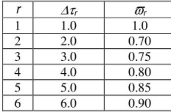
ϖ(τ) = ϖr, β(τ) = β,r , τr−1≤τ≤τr, r = 1 : R.
If ϖ(τ) happens to be equal to 1 for some τ in the interval [τr-1 ,τr]
then, ϖ(τ) = 1 everywhere in [τr-1 ,τr], and therefore ϖr = 1. In this
sense, we may think of a “conservative layer”, and we are giving an alternative definition (perhaps more adequate at this point) for a multislab conservative problem: a multislab problem is conservative if at least one layer is conservative. It is non-conservative otherwise. Continuing, the depth-dependent anisotropic source that appears in Eq. (15) can be expressed as
.) ( ) ( ) 1 2 ( 2 ) ( 1 exp ) , (
0
0 , 0
0
0
∑
∞
=
+
− −
= τ τ ϖ β µ µ
µ µ
τ I P P
s r
r u
r (17)
Result (17) can be written in the shorter form
, : 1 , ,
1 1 , ) ( 1 exp ) ( ) ,
( 0 1
0 0
R r s
s r r r
u
r − ≤ ≤ ≤ ≤ =
− −
= µ µ τ τ µ τ− τ τ
µ
τ (18)
where
.) ( ) ( ) 1 2 ( 2 ) (
0 , 0
0
0
∑
∞= +
≡ ϖ β µ µ
µ I P P
s r
r
r (19)
We follow by considering standard SN approximations (Lewis and Miller Jr., 1993) to the local diffusive equations (15) of the form
, : 1 , ,
: 1 ), (
) ( ) ( ) ( ) 1 2 ( 2 ) ( ) (
1 ,
0 , 1 ,
, ,
R r N
m s
I P P
I I d
d
r r u
m r
r
L N
n
d n r n n m r r
d m r d
m r m
= ≤ ≤ =
+
+ =
+
−
= =
∑
∑
τ τ τ τ
τ µ ω µ β ϖ
τ τ τ
µ (20)
where
) , ( ) (
, m
d r d
m
r I
I τ ≅ τ µ , , ( ) ( , m)
u r u
m
r s
s τ ≅ τ µ ,
and {µm}, m = 1 : N, is a finite set of angular directions on the
interval [-1,1]. In this article, we consider even-order Gauss-Legendre quadrature sets (Lewis and Miller Jr., 1993). That is to say, the directions µm, m = 1 : N, are the roots of the Nth-degree
Legendre polynomial PN(µ), and the angular weights ωn , n = 1 : N,
are so that the quadrature formula on the right side of the equal sign in Eqs. (20) integrates exactly Legendre polynomials from P0(µ) to
P2N-1(µ). We remark that we have ordered the directions µm so that µm> 0 holds for m = 1 : N/2, µm< 0 holds for m = N/2+1 : N, where µm-1 < µm, m = 2 : N/2 and µm+N/2 = –µm, m = 1 : N/2. We remark also
that the nonnegative integers Lr in Eqs. (20), r = 1 : R, indicate that
the Legendre expansions of the scattering phase functions in corresponding layers have been truncated after (Lr+ 1) terms. We
note further that intensity continuity conditions still hold at layer interfaces, and that we have used the standard discrete boundary conditions (Lewis and Miller Jr., 1993)
, , ) ( I ); ( ) (
I1d,m τ0 =γ0 µm Rd,−m τR =0 µm >0 21)
where the subscript –m is to denote the angular direction –µm.
Solution to the SN system (20) can be expressed for each r in terms of the solution to the homogeneous version of Eqs. (20), and a particular solution in the vector form
, ),
( I ) ( I ) (
I , 1
1 , , r r
d p r N
i d
i r i r d
r τ = α τ + τ τ − ≤τ ≤τ
=
∑
(22)where
; )] ( I , ), ( I ), ( I [ )
( rd, rd, dr,N T
d
r τ ≡ 1τ 2τ τ
I
αr,i , i = 1 : N, are scalars depending upon the discrete boundary
conditions (21);
, ,
N : i , )] ( I , ), ( I ), ( I [ )
( rdi,, rd,i, rd,i,N T r r
d i ,
r τ ≡ 1τ 2τ τ =1 τ −1≤τ≤τ
I (23)
are the elements of a vector basis for the null space of the local SN radiative transfer operator
, : 1 , ) )( ( ) ( ) 1 2 ( 2 ) ( 1
0 , 1
N m P P
d
d Lr N
n n n m r r
m • − + • =
+
∑
∑
= β µ =ω µ
ϖ τ
µ (24)
where (•) denotes appropriate operations on the entries of vector (23), and
. ,
)] ( I , ), ( I ), ( I [ )
( dr,p, rd,p, rd,p,N T r r d
p ,
r τ ≡ 1τ 2 τ τ τ −1≤τ≤τ
I (25)
, : 1 , : 1 , ,
exp ) ( )
( 1
, , ,
, ,
, a i N m N
I r r
i r
i r i
r m r d
m i
r ≤ ≤ = =
−
= ν τντ τ − τ τ
τ (26)
where τr,i, i = 1 : N, are appropriate depths. The quantities νr,i and ar,m(νr,i), are the separation constants and the angular components
(de Abreu, 1998; Siewert, 2000) of the elementary solutions (26), respectively.
We now show that the natural choice (26) implies that the vector basis with elements (23) is a basis of eigenvectors of an auxiliary local SN operator. For so we substitute the exponential solutions (26) into the homogeneous version of the SN Eqs. (20), we first order operate on the left side of the equal sign and we obtain
. : 1 ,
, exp
) ( ) ( ) ( ) 1 2 ( 2
exp ) ( exp
) (
1
0 1 ,
, ,
, ,
, , ,
, ,
, ,
, ,
N m
a P P
a a
r r r
L N
n ri
i r i
r n r n n m r r
i r
i r i
r m r i r
i r i
r m r i r
m
= ≤ ≤
−
+
=
−
+
−
−
= =
∑
∑
τ τ τ
ν τ τ ν µ ω µ β ϖ
ν τ τ ν ν
τ τ ν ν
µ
(27)
Equations (27) can be reformulated further and be cast in the matrix form
) ( )
(
A r r,i
i , r i , r
i , r i
, r r r i , r
i ,
r ν
ν ν
τ τ ν
ν τ τ
a
a exp 1
exp
−
=
−
(28)
or, equivalently,
, ) ( ) (
A d
i , r i , r d
i , r
rI τ ν I τ
1
= (29)
where the operator Ar on the left side of the equal sign in Eq. (29) is an auxiliary SN (matrix) operator with entries
, : 1 , : 1 , ) ( ) ( ) 1 2 ( 2 1
0 ,
, P P m Nn N
A n
r L
n m r r
mn m r
n
m = =
+ +
−
≡
∑
= β µ µ ω
ϖ δ
µ (30)
where δmn is the Kronecker delta and
. N : i , )] ( a , ), ( a ), ( a [ )
( r,i r, r,i r, r,i r,N r,i T
r ν ≡ 1ν 2 ν ν =1
a (31)
Equation (29) is an eigenvalue problem defined by the auxiliary local SN operator Ar. The eigenvalues (νr,i)-1, i = 1 : N, of operator Ar
are the reciprocals of the separation constants νr,i and the
corresponding eigenvectors are the basis vectors (23) with entries given by (26). Therefore, the vector basis for the null space of operator (24) with elements (23) and entries (26) is a basis of eigenvectors of the auxiliary local SN operator Ar. But nothing has
been said until now about the existence of such basis of eigenvectors. We discuss this very important point next.
For an oriented discussion of the existence for the null space of operator (24) of a basis of eigenvectors of the auxiliary operator Ar,
we shall step back a bit to state some preliminary results and to make a relevant assumption. We begin by dividing Eqs. (27) by the function exp [(τ – τr,i) / νr,i], and we notice that the resulting
-dependent, N-term series on the right side of the equal sign is just the zeroth-order th-degree Chandrasekhar polynomial (1950) evaluated at νr,i. Then, we may write
. : 1 , ) ( ) ( ) 1 2 ( 2 ) ( ) (
0 ,
0 , , ,
, , , ,
N m g P a
a
r L
i r r m r r
i r m r i r m r i r
m + =
∑
+ == β µ ν
ϖ ν ν
ν
µ (32)
Now, with the parity relations
P (–µm) = (–1) P (µm) andg0r,(−νri,)=(−1) gr0,(νri,)
for Legendre (Lewis and Miller Jr., 1993) and Chandrasekhar (1950) polynomials, respectively, it is not difficult to draw that the separation constants appear in ± pairs of numbers and that the angular components satisfy the relation ar,m(νr,i) = ar,–m(–νr,i) for all r, m and i. In this article, we assume that the ± pairs of separation constants are distinct and real. The relationship for the angular components will be brought to further discussion only in the final section of this article. Let us make use of the former result (± pairs of numbers) and of our assumption (distinct real) to discuss the existence of a basis of eigenvectors of operator Ar. If the separation
constants are bounded, i.e. there exists a positive real number K so that |νr,i| < K for all i, then zero is not at all an eigenvalue of Ar, viz
Eq. (29). Since the separation constants are distinct pairs of ± real numbers and zero is not an eigenvalue of Ar, the eigenvalues of Ar
form a distinct set of real numbers. This implies that there exists a basis of eigenvectors of Ar (Schneider and Barker, 1989). Numerical
evidence (Shultis and Hill, 1976; Siewert, 1978, 2000) indicates that this is true of non-conservative layers (0 ≤ ϖr < 1). On the other
hand, it is known (Chandrasekhar, 1950; Case and Zweifel, 1967; Benassi et al., 1984; Siewert, 2000) that, for conservative layers, there exists a ± pair of unbounded constants satisfying for example Eqs. (27). Therefore, the auxiliary local SN operator Ar has a zero
eigenvalue with algebraic multiplicity (Schneider and Barker, 1989) equal to 2 (a double zero eigenvalue), viz Eq. (29). Unfortunately, the operator Ar has no special properties (to our knowledge) to
guarantee that the geometric multiplicity (Schneider and Barker, 1989) of the double zero eigenvalue be also equal to 2. So, for the conservative case ϖr = 1, the operator Ar may not provide a basis of
eigenvectors for the null space of the local SN operator (24). But even so we can do the following: when generating the eigenvalues and corresponding eigenvectors of the auxiliary local SN operator Ar
and for ϖr = 1, we simply discard the eigenvector(s) corresponding
to the double zero eigenvalue and replace it (them) with a pair of vectors of the form (23) belonging to the null space of the local SN operator (24). These replacing vectors have entries given by the elementary solutions
,m :N,
) ( ) (
r , r
m
r
r 1
1 1
= − + −
β τ ∆
µ τ
∆ τ
τ (33)
and
, N : m , ) ( ) (
r , r
m
r
r 1
1 1
1 =
− −
− −
β τ ∆
µ τ
∆ τ
τ (34)
respectively, with ∆τr ≡ τr – τr-1 and |β1,r| < 1 for all r. The
elementary solutions (33-34) are SN variants to elementary solutions of the homogeneous integrodifferential transfer equation reported on page 14 of the book of Chandrasekhar (1950) for the conservative case (the reader may check solutions (33-34) against the homogeneous version of the SN Eqs. (20)). Similar solutions are also reported in the Appendix F of Case and Zweifel (1967) for neutron transport problems but for isotropic scattering (β1,r = 0 in this case).
Elementary solutions very similar to (33-34) can also be found in a recent work by Siewert (2000).
. : 1 , ,
exp )
( 1
0 ,
,
, f m N
Irdpm rm r ≤ ≤ r =
−
= µτ τ − τ τ
τ (35)
The exponential functions (35) are SN versions of the particular solution used by Chandrasekhar (1950) to express the solution to the classical albedo problem in radiative transfer, and fr,m , m = 1 : N,
are constants to be determined upon substitution of functions (35) into Eqs. (20). As noted by Siewert (2000) in a recent work, the exponential functions (35) are not valid in the (unlikely) event that
µ0 be equal to one of the separation constants νr,i , i = 1 : N. So, we
are assuming here that µ0 does not match any νr,i for all i. The
constants fr,m, m = 1 : N, in the exponential functions (35) can be
efficiently computed with the help of the parity relation for the Legendre polynomials and through a not-so-straightforward use of matrix algebra for splitting and handling the matrix equation resulting from the substitution of the exponential functions (35) into the SN Eqs. (20). An outline of this technique follows. For fixed r, the constants fr,m , m = 1 : N, are the entries of the
(N/2)-dimensional column matrices
(
)
(
)
(
)
(
)
+ −
+ + −
−
= − − −
+
r r r r r r
r r r r
r M FE d Fc EF c Ed
f 0
1 2 0 0
1 2 0 1 0
Ι
Ι
2
1µ µ µ µ µ (36)
and
(
FE)
(
F)
(
EF)
(
E)
,M r r r r r r r r r r
r
+ −
− + −
−
= − − −
− d c c d
f 0
1 2 0 0
1 2 0 1 0
Ι
Ι
2
1µ µ µ µ µ (37)
where
[
]
T/ N , r , r
r+≡ f 1; ;f 2
f (38)
and
fr− ≡
[
fr,N/2+1; ;fr,N]
T, (39)respectively. The quantities
1
Ι + − −
+ −
≡[ (T T)]M
Er r r and 1
Ι + − −
− −
≡[ (T T)]M
Fr r r
are (N/2)-dimensional real square matrices. The symbol I is to denote the (N/2)-dimensional identity matrix and M is the (N/2)-dimensional diagonal matrix whose entries are Mii = µi, i = 1 : N/2.
The quantities Tr+ and Tr− denote (N/2)-dimensional real square matrices with entries
(2 1) ( ) ( ) , 1: /2, 1: /2,
2 0 ,
,
, P P m N n N
T n
r L
m r r
n n m
r = =
+
=
∑
=
+ ω ϖ β µ µ (40)
and
, 2 / : 1 , 2 / : 1 , ) ( ) ( ) 1 ( ) 1 2 (
2 0 ,
,
, P P m N n N
T n
r L
m r r
n n m
r = =
− +
=
∑
=
− ω ϖ β µ µ (41)
respectively. The quantities cr and dr in results (36-37) are (N/2)-dimensional column matrices given by
[
]
TN , r / N , r /
N , r , r / N , r ,
r s ;s s ; ;s s
s01+ 0 2+1 02+ 0 2+2 0 2+ 0 (42)
and
[
sr0,1−sr0,N/2+1;s0r,2−s0r,N/2+2; ;sr0,N/2 −sr0,N]
T, (43) respectively.From the foregoing analysis, we may draw a number of conclusions important to define and substantiate the method to be described in the next section. Firstly, if I0 = 0 and the boundary function γ0(µ) ≠ 0, then we draw from result (13) that Iu(τ,µ) = 0 everywhere in Ω and for all µ, from result (14) that su(τ,µ) = 0 everywhere in Ω and for all µ and from results (36) through (43) that the constants fr,m = 0, for all r and for m = 1 : N. Therefore, the
exponential functions (35) are zero everywhere in the real interval [τr-1 ,τr] for all r and the particular solution vector (25) is the null
vector of the null space of operator (24). In this case, solution to the target problem (1-3) in each of the discrete directions in the finite set {µm}, m = 1 : N, is approximately given by the open form
solution (22). This should not be surprising, for the resulting target problem is just the diffusive problem (6-7) with su
(τ,µ) = 0, which
has been formulated and approximately solved with our previous SN
analytical and numerical methods. On another hand, if I0≠ 0 and the boundary function γ0(µ) = 0 then, formulation and analysis provided here are mathematically equivalent to those recently reported by us (de Abreu, 2004) for problems with only a monodirectional beam. Therefore, a mathematical method founded in the results derived in the foregoing analysis may be expected to work with both one-type (singular or regular) and mixed boundary conditions. Secondly, the scalars αr,i are hitherto unknown quantities. This is a call for one of
the open questions in our preceding analysis – the determination of the scalars αr,i in all layers of the multislab domain Ω, and we intend
to address an appropriate reply in the coming section. Thirdly, even with the scalars αr,i on hand, the best we can do with available
information is to close up the open form solution (22) and add it to the closed solution (13) to yield an approximate solution to the target problem (1-3) only in the discrete directions considered in the SN Eqs. (20). In the preceding analysis, nothing has been said about a way of obtaining approximate solutions to the local diffusive equations (15) that are continuous in τ and µ. This gap is bridged
with the equivalence between the SN formulation considered in this
article and an angularly continuous formulation classical in radiation transport theory.
At this point, we proceed to describe a mathematical method for an approximate solution to the target problem (1-3).
A Mathematical Method for Solving the Target Problem The mathematical method described in this section is a conjugation of basic relations from more general results in the theory of radiation transport and a two-component method based on recently developed SN analytical and numerical methods for an approximate solution to the target problem (1-3). The approximate solution we seek is a distribution on τ and µ of the form
, ,
), , ( I ) , ( I ) , (
INτ µ = u τ µ + Nd−1τ µ τ0≤τ≤τR −1≤µ≤1 (44)
where Iu(τ,µ) means that we have directly incorporated the closed form (13) into our approximate solution, and the second term on the right side of the equal sign in (44) denotes the well-known spherical harmonics (PN-1) approximation (Duderstadt and Martin, 1979; Lewis and Miller Jr., 1993) to the solution of the diffusive Eqs. (15) given by
, : 1 , 1 1 , ,
) ( ) ( 2
) 1 2 (
) , (
1 1
0 ,
1
R r P
I
r r N
d r d
N
= ≤ ≤ − ≤ ≤ +
=
− −
= −
∑
φ τ µ τ τ τ µ µτ
where
R : r , ,
N : m ), ( I ) , (
INd−1τµm = rd,mτ =1 τr−1≤τ≤τr =1 .
The quantities
, : 1 , ,
) ( ) ( )
( 1
1 ,
, P I r r r R
N
t
d t r t t d
r = − ≤ ≤ =
=
∑
ω µ τ τ τ ττ
φ (46)
are the PN-1 angular moments (Duderstadt and Martin, 1979; Lewis
and Miller Jr., 1993) of the diffuse component of the intensity of the radiation field. Results (45) and (46) can be shown to come up from two different and equivalent formulations of the diffusive problem (6-7) – the SN formulation composed by the SN Eqs. (20) and the discrete boundary conditions (21) and the classical PN-1 formulation with the corresponding boundary conditions due to Mark (Davison, 1957; Duderstadt and Martin, 1979). Expressions (44-46) constitute the basic relations of the mathematical method described in this section. We should note that the diffuse component (45) of our approximate solution (44) is continuous in τ and µ on Ω. We note further that the only unknown quantities in expressions (44-46) are the entries of the SN solution vector (22), which will be provided by
a two-component method based on recently developed SN analytical
and numerical methods.
As the name implies, our two-component method has two ingredients: a numerical component and an analytical component. The numerical component is to provide layer-average
, R : r , N : m , d ) ( I I
r
r
d m , r r d
m ,
r 1 1
1
1
= =
≡
∫
− τ
τ
τ τ τ
∆ (47)
and layer-edge values for the entries of the SN solution vector (22)
without having to determine the scalars αr,i, r = 1 : R, i = 1 : N, in
the open form (22). The numerical component is thus suited to radiative transfer problems where the quantities of interest are, for example, the angular distribution of radiation leaving the multislab domain and angle-integrated layer-edge quantities such as radiative heat fluxes (Chandrasekhar, 1950; Thomas and Stamnes, 1999). For the angular distribution of leaving radiation, we make direct use of results (46) through (44) at τ = τ0 for µ < 0 and at τ = τR for µ > 0.
For layer-edge radiative heat fluxes, we may use expression (46) at
τj, j = 0 : R, to get approximations for the downward (+) and upward
(–) partial fluxes
, 2
1 2
) 1 ( 2
) 1 ( ) ( 2
) 1 2 (
exp
) , ( )
, ( )
, (
2 / ) (
1 1
0 ,
0 0 0
0
1
0 1 1
0 1
0
∑
∑
∫
∫
∫
= −
=
±
− ±
+ +
± +
+
−
−
= ± +
± =
±
=
N
m
m m
m N
j d r
j
j d N j
u j
N
j N
P I
H
d I
d I
d I
q
µ µ
ω τ
φ
µ τ τ µ
µ µ τ µ µ µ τ µ µ µ τ µ
π τ
(48)
where H± is the unit step function (H+= 1 and H−= 0), as well as for the net fluxes
). ( ) ( )
( j N j N j
N q q
q τ = +τ − − τ (49)
The analytical component of our two-component method is to reconstruct the approximate solution (44) by solving a system of
linear algebraic equations for the scalars αr,i in the SN solution (22). Inputs to the system are layer-edge values for Ird,m(τ) supplied by
the numerical component. The analytical component is to be applied when the intensity of the radiation field IN(τ,µ) at any depth τ and
direction µ is sought, for then we make use of results (22) and (46) back to (44). We remark that, with the scalars αr,i determined, the
radiative heat fluxes (48-49) can also be obtained at any depth τ
through results (22) and (46). We describe next either component. The numerical component of our two-component method is a numerical method designed for solving the SN diffusive problem (20-21) with no optical truncation error. That is to say, the numerical solution of the SN diffusive problem (20-21) generated by our numerical method agrees to the analytical solution (22) on corresponding layer-edge points, apart from computational finite arithmetic considerations and regardless of the optical thicknesses of the layers forming the multislab domain. Our numerical method is an extension to anisotropic scattering of arbitrary (Legendre) order and to depth-dependent anisotropic sources of the former spectral Green’s function (SGF) method for neutron transport problems (Barros and Larsen, 1990). For this reason, we refer to our numerical method as the extended spectral Green’s function (ESGF) method.
The ESGF method has two main ingredients: one is standard and the other is nonstandard. The standard ingredient is the derivation of the local radiative balance equations
, : 1 , : 1 , )
( ) ( ) 1 2 ( 2
) (
,
0 , 1 ,
, , 1 ,
N m R r s I P P
I I I
u m r r
L N
n
d n r n n m r r
d m r d
m r d
m r r m
= = + +
= + −
∑
∑
= =
−
µ ω µ β ϖ
τ ∆
µ
(50)
where Idj,m≡Ird,m(τj),j = r-1 : r, r = 1 : R,
are layer-edge intensities;
, s
) ( s d
s r r
r m , r u
m , r r u
m , r
r
r
− −
− =
≡
∫
−− 0 0
1 0
0 exp exp
1
1 µ
τ µ
τ τ
∆µ τ
τ τ ∆
τ
τ
(51)
and d
m , r
I , r = 1 : R, m = 1 : N, is given by definition (47). The local
balance Eqs. (50), together with the discrete boundary conditions (21), form a system of linear algebraic equations whose unknowns are layer-average and layer-edge intensities. Such a system does not have a unique solution because there are more unknowns than equations. A simple count gives us N(R+1) layer-edge intensities, NR layer-average intensities, NR balance equations and N boundary
equations. The net score is N(2R+1) unknowns against N(R+1)
equations. Therefore, N(2R+1) – N(R+1) = NR additional equations are needed or, equivalently, N additional equations per layer relating layer-edge and layer-average intensities.
The nonstandard ingredient is to provide NR equations to the system of N(R+1) equations referred to in the preceding paragraph. These NR additional equations are the ESGF auxiliary equations
, : 1 , : 1 , , 1
2 / , , , 2
/
1 , , 1,
, I I g r Rm N
I rm
N
N u
d u r u m r N
u d
u r u m r d
m
r =
∑
+∑
+ = =+ =
= θ − θ
(52)
where the layer-dependent coefficients θr,m,u and gr,m are determined
in a layer-by-layer process in order that the analytical solution (22) do satisfy the ESGF auxiliary Eqs. (52), for arbitrary scalars αr,i and
exponentials) or conservative (two vectors have polynomial entries and the remaining vectors have exponential entries), our presentation will be oriented by layer type. So, let us consider a layer in the multislab domain Ω and let us calculate the layer-average intensities in terms of analytical results derived in the preceding section. If the target layer is non-conservative, then we consider the SN analytical solution (22) with the entries of all basis vectors (23) given by (26), we substitute the entries of (22) into definition (47) and, after some Calculus, we obtain
, exp exp exp exp ) ( 0 0 1 , 0 1 , , 1 , , , , , , , − − − + − − − = − = −
∑
µ τ µ τ τ ∆ µ ν τ τ ν τ τ τ ∆ ν ν α r r r m r Ni ri
i r r i r i r r r i r i r m r i r d m r f a I (53)
for m = 1 : N. However, if the target layer is conservative, we shall consider that two basis vectors (23) have entries given by the elementary solutions (33) and (34), respectively, and the remaining vectors have entries given by (26). If we tag these two basis vectors with i = 1 and i = 2, and if we proceed as in the non-conservative case, then we can obtain
. : 1 , exp exp exp exp ) ( ) 1 ( 2 1 ) 1 ( 2 1 0 0 1 , 0 3 , , 1 , , , , , , , 1 2 , , 1 1 , , N m f a I r r r m r N
i ri
i r r i r i r r r i r i r m r i r r r m r r r m r d m r = − − − + − − − + − − + − + = − = −
∑
µ τ µ τ τ ∆ µ ν τ τ ν τ τ τ ∆ ν ν α β τ ∆ µ α β τ ∆ µ α (54)Since the ESGF auxiliary Eqs. (52) are to be satisfied by the SN analytical solution (22) for arbitrary scalars αr,i, for the entries of the
particular solution vector (25) given by the exponential functions (35), and for every layer in the multislab domain, we can substitute result (53) and the entries of the analytical solution (22) (with entries (26) for the basis vectors (23)) evaluated at τr-1 and τr into the
ESGF auxiliary Eqs. (52) to obtain for a non-conservative layer the SN equations
, exp exp ) ( exp exp ) ( exp exp ) exp ) exp ) ( , 1 2
/ 1 , , 0
, , , , , , 2 / 1 0 1 , 1 , , 1 , , , , , 0 0 1 , 0 1 , , 1 , , , , , , m r N N u r u r N
i ri
i r r i r u r i r u m r N u r u r N
i ri
i r r i r u r i r u m r r r r m r N
i ri
i r r i r i r r r i r i r m r i r g f a f a f a + − + − + − + − = − − − + − − −
∑
∑
∑
∑
∑
+ = = = − = − − = − µ τ ν τ τ ν α θ µ τ ν τ τ ν α θ µ τ µ τ τ ∆ µ ν τ τ ν τ τ τ ∆ ν ν α (55)for m = 1 : N. For a conservative layer, we proceed similarly to get
. : 1 , exp exp ) ( ) 1 ( 1 ) 1 ( exp exp ) ( ) 1 ( ) 1 ( 1 exp exp exp exp ) ( ) 1 ( 2 1 ) 1 ( 2 1 , 0 , 3 , , , , , 1 2
/ , , ,1 1, ,2 1,
0 1 , 3 , , 1 , , , 2 /
1 , , ,1 1, ,2 1,
0 0 1 , 0 3 , , 1 , , , , , , , 1 2 , , 1 1 , N m g f a f a f a m r r u r N
i ri
i r r i r u r i r N N
u r r
u r r r u r u m r r u r N
i ri
i r r i r u r i r N
u r r
u r r r u r u m r r r r m r N
i ri
i r r i r i r r r i r i r m r i r r r m r r r m r = + − + − + − − + − + − + − + − − + − + = − − − + − − − + − − + − +
∑
∑
∑
∑
∑
= + = − = − = − = − µ τ ν τ τ ν α β τ ∆ µ α β τ ∆ µ α θ µ τ ν τ τ ν α β τ ∆ µ α β τ ∆ µ α θ µ τ µ τ τ ∆ µ ν τ τ ν τ τ τ ∆ ν ν α β τ ∆ µ α β τ ∆ µ α (56)Since Eqs. (55-56) hold for arbitrary scalars αr,i , they hold for αr,i
set equal to zero for all i from 1 to N. This yields the coefficients
, : 1 , exp exp exp exp 1 2 / , , , 0 2 /
1 , , ,
0 1 0 0 1 , 0 , N m f f f g N N u u r u m r r N u u r u m r r r r r m r m r = − + − − − − − =
∑
∑
+ = = − − θ µ τ θ µ τ µ τ µ τ τ ∆ µ (57)in either case (conservative and non-conservative). We substitute result (57) into Eqs. (55-56), we cancel equivalent terms out on both sides of the equal sign and we arrive at
, ) ( exp ) ( exp exp exp ) ( 1 2 / , , , , , , 2 /
1 , , , ,
, , 1 1 , 1 , , 1 , , , , , , − + − = − − −
∑
∑
∑
∑
+ = = − = = − N N u i r u r u m r i r i r r N u i r u r u m r i r i r r N i i r Ni ri
i r r i r i r r r i r i r m r i r a a a ν θ ν τ τ ν θ ν τ τ α ν τ τ ν τ τ τ ∆ ν ν α (58)
for a non-conservative layer, and
, ) ( exp ) ( exp ) 1 ( 1 ) 1 ( ) 1 ( ) 1 ( 1 exp exp ) ( ) 1 ( 2 1 ) 1 ( 2 1 1 2 / , , , , , , 2 /
1 , , , , , , 1 3 , 1 2
/ , , 1,
2 /
1 , , 1,
2 ,
1 2
/ , , 1,
2 /
1 , , 1,
1 , 3 , , 1 , , , , , , , 1 2 , , 1 1 , − + − + − − + − − + − + − + = − − − + − − + − +
∑
∑
∑
∑
∑
∑
∑
∑
+ = = − = + = = + = = = − N N u i r u r u m r i r i r r N u i r u r u m r i r i r r N i i r N Nu r r
u u m r N
u r r
u u m r r N N
u r r
u u m r N
u r r
u u m r r N
i ri
i r r i r i r r r i r i r m r i r r r m r r r m r a a a ν θ ν τ τ ν θ ν τ τ α β τ ∆ µ θ β τ ∆ µ θ α β τ ∆ µ θ β τ ∆ µ θ α ν τ τ ν τ τ τ ∆ ν ν α β τ ∆ µ α β τ ∆ µ α (59)
for a conservative one, with m = 1 : N. Since Eqs. (58-59) hold for arbitrary scalars αr,i , they must hold for the N ordered sets of scalars
(δ1j, δ2j, δ3j, …, δNj), j = 1 : N. These ordered sets of scalars yield,