A. Campos
R. Guenther
and D. Martins
Universidade Federal de Santa Catarina Departamento de Engenharia Mecânica Laboratório de Robótica Caixa Postal 476 Campus Universitário – Trindade 88040 900 Florianópolis, SC. Brazil [email protected] [email protected] [email protected]
Differential Kinematics of Serial
Manipulators Using Virtual Chains
This paper presents a new approach to calculate the direct and inverse differential kinematics for serial manipulators. The approach is an extension of the Davies method for open kinematic chains based on a virtual kinematic chain concept introduced in this paper. It is a systematic method that unifies the kinematics of serial manipulators considering the type of kinematics and the coordinate system of the operational space and constitutes an alternative way to solve the differential kinematics for manipulators. The usefulness of the method is illustrated by applying it to an industrial robot.Keywords: Robot analysi, differential kinematics, screw theory
Introduction
Kinematics is a branch of physics concerned with the geometrically possible movements of a body or a system of bodies without considering the forces and masses involved.
Robot manipulator kinematics deals with the movements of the robot end-effector and how the robot joints need to move, in a coordinate manner, to achieve the end-effector prescribed movement. 1
Differential kinematics relates the velocities of the manipulator components. These velocities may be the velocities at the joints of the manipulator or the velocities of one or more links in the manipulator kinematic chain. The standard approach to differential kinematics is to relate joint and end-effector velocities through the Jacobian matrix, which allows the calculation of the end-effector velocities given the joint velocities (direct differential kinematics) or, to determine the joint velocities in order to move the end-effector with a prescribed speed (inverse differential kinematics).
Another important feature of differential kinematics is the singularity analysis, commonly based on the Jacobian matrix.
Furthermore, differential kinematics is used to define indices for the evaluation of the manipulator performance (Sciavicco, 1996),
e.g. manipulability ellipsoids (Angeles, 1997). Such indices, also known as quality indices (Downing, 2002), may be helpful both for the mechanical manipulator design and for determining suitable manipulator configurations to execute a given task.
In the literature, the differential kinematics of robots with serial kinematic chains (serial robots for short) is described using variations of two main approaches: the method based on Denavit-Hartenberg parameters (Sciavicco, 1996) and the screw-based method (Hunt, 1987; Duffy, 1996; Davidson and Hunt, 2004). The latter allows the expression of the Jacobian manipulator in a greatly simplified manner by expressing the screws in a properly chosen reference frame (Tsai, 1999).
In both descriptions the direct differential kinematics is usually obtained by calculating the Jacobian and, after this, the inverse kinematics is obtained by inverting the Jacobian matrix.
This paper presents a new variation of the screw-based method that allows the determination of the direct and the inverse differential kinematics using a single systematic approach.
This approach is derived from the Davies formulation of the Kirchhoff law, here designated as the Davies method (Davies, 1981,
Paper accepted July, 2005. Technical Editor: José Roberto de França Arruda.
1983). The Davies method uses the differential kinematics screw representation, as described below for completeness.
The Davies method allows the calculation of the differential kinematics of closed kinematic chains by relating the joint rates along the chain. By considering that closed kinematic chains have actuated joints (with known velocities) and passive joints (in which the velocities will be calculated), it may be stated that, more specifically, the Davies method is a systematic way to express the joint rates of passive joints as functions of the joint rates of the actuated joints.
The Davies method, very useful for analyzing mechanical networks with multi-loop kinematic chains, has, however, two drawbacks when applied to robot kinematics. First, it is limited to fully closed kinematic chains; therefore, it is not possible to apply this method to solve the differential kinematics of serial robots (open kinematic chains). Second, the method cannot be used to obtain information about the rigid body movement of a specific link, e.g. the robot end-effector in a desired operational space (Cartesian, cylindrical etc.).
This paper formalizes the concept of a virtual kinematic chain as suggested by Davies (Davies, 2000) and shows that by using this concept it is possible to overcome the Davies method drawbacks mentioned above and to extend the method to robot kinematics in order to calculate its direct and inverse differential kinematics using the same single systematic approach.
Furthermore, it allows the determination of the inverse differential kinematics in a coordinate system (Cartesian, cylindrical etc.) suitable for the end-effector task, which is not so evident to be achieved using conventional methods.
This paper has the following structure. Initially, the differential kinematics of a body is represented using screws. Next, the Davies method and the joint space kinematic solution are described. Then, the concept of a virtually modified chain and its properties are proposed. Following this, the joint space kinematics for a virtually modified chain is solved. Finally, the differential kinematics using virtual chains is discussed and the direct and inverse differential kinematics for a PUMA serial manipulator is calculated using the proposed method for a Cartesian and a cylindrical operational space.
Nomenclature
$= screw movement or twist h = pitch of the screw Vp= linear velocity of point p
SO= position vector of any point at the screw axis
S = normalized vector parallel to screw axis N = matrix containing the normalized twists Fb =gross degree of freedom
FN =net degree of freedom
d =order of the screw system
n =number of links of a kinematic chain f =degree of freedom of a kinematic pair
m =rank of matrix containing the normalized twists T = transformation matrix of screw coordinates R = rotation matrix
W = skew-symmetric matrix representing a vector
Greek Symbols
ω
= differential rotation about the screw axis, angular velocity
τ
= differential translation along the screw axis, linear velocity
Ψ
= twist magnitude
θ
= position angles at the rotary joints Subscripts
s relative to secondary
p relative to primary
i,j relative to link or joint i,j
Screw Representation of Differential Kinematics
The Mozzi theorem (see Ceccarelli, 2000, for the original quotation and historical remarks) states that the velocities of the points on a rigid body with respect to an inertial reference frame
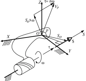
O(X,Y,Z) may be represented by a differential rotation ω about a certain fixed axis and a simultaneous differential translation τ along the same axis. The complete movement of the rigid body, combining rotation and translation, is called screw movement or twist $. Fig. 1 shows a body “twisting” around an axis instantaneously fixed with respect to the inertial reference frame. This axis is called the screw axis and the ratio of the linear velocity and the angular velocity is called the pitch of the screw h= ||τ ||/||ω ||.
τ
ω
O
$
X
Y Z
Figure 1. Screw movement or twist.
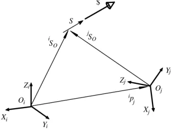
The twist represents the differential movement of the body with respect to the inertial frame and may be expressed by a pair of vectors, i.e. $=(ω ;Vp). The vector ω =(L, M, N ) represents the angular velocity of the body with respect to the inertial frame. The vector Vp=(P*, Q* ,R*) represents the linear velocity of a point P
attached to the body which is instantaneously coincident with the origin O of the reference frame (see Fig. 2).
The vector Vp consists of two components: a) a velocity parallel
to the screw axis represented by τ =hω ; and b) a velocity normal to the screw axis represented by SOxω , where S
O is the position vector
of any point at the screw axis.
$ xω
τ= ω
τ
ω
So o
S
X
Y
O p
Z h
S Vp
Figure 2. Twist components for a general screw kinematic pair.
A twist may be decomposed into its amplitude and its corresponding normalized screw. The twist amplitude Ψis either the magnitude of the angular velocity of the body, ||ω ||, if the kinematic pair is rotative or helical, or the magnitude of the linear velocity, ||Vp||, if the kinematic pair is prismatic. Consider a twist
given by $=(ω ;V
p)
T
= (L, M, N ;P*, Q* ,R*)T. Then, the correspondent
normalized screw is $ˆ =(L, M, N; P*, Q* ,R* )T. This normalized
screw is a twist in which the magnitude Ψis factored out, i.e.
Ψ =$ˆ
$ (1)
The normalized screw coordinates (Davidson and Hunt, 2004) may be defined as a pair of vectors, namely, (L,M,N) and (P*,Q*,R*), given by,
+ × =
=
S S S
S
O h
R Q P N M L
* * *
$ˆ (2)
where S is the normalized vector parallel to the screw axis. Notice that the vector (SO×S)determines the moment of the screw axis
with respect to the origin of the reference frame.
The movement between two adjacent links, belonging to an n-link kinematic chain, may also be represented by a twist. In this case, the twist represents the movement of link i with respect to link (i-1).
In Robotics, generally, the movement between a pair of bodies is determined by either a rotative or a prismatic kinematic pair.
× =
S S
S
O
$ˆ (3)
For a prismatic pair the pitch of the twist is infinite (h=∞) and the normalized screw reduces to
=
S
0
$ˆ (4)
Often it is useful to represent the differential movement of a body, expressed by a twist $, in different reference frames. In what follows, a 6 x 6 matrix of transformation T to serve this purpose is presented (Tsai,1999).
Consider two reference frames of interest (Xi,Yi,Zi) and (Xj,Yj,Zj)
as in Fig. 3.
S
Oi
S
Oj
p
iS
$
Z
jX
jO
jX
Y
Z
O
i
i i
i
Y
jj
Figure 3. Coordinate transformation of a screw.
The position of origin Ojrelative to the (Xi,Yi, Zi) frame is given
by ip
j=[px,py,pz] T
and the orientation of the (Xj,Yj,Zj) frame relative
to the (Xi,Yi,Zi) frame is described by a rotation matrix iRj. A screw
represented in the (Xi,Yi, Zi) frame is denoted by i$, and the same
screw represented in the (Xj,Yj,Zj) frame is denoted by j$.
Following the normalized screw definition, we have
+ × =
S S S
S
O
i i i
i i
h
$ˆ (5)
+ × =
S S S
S O
j j j
j j
h
$ˆ (6)
The line vectors S and the moment vectors SOof the two screws
are related by the following transformations:
O
O S
S
S S
j j i j i i
j j i i
R p
R + =
=
(7)
Hence
$ˆ j$ˆ
j i i
T
= (8)
where
=
j i j i j i
j i
j i
R R W
R
T 0 (9)
is a 6 x 6 matrix, and
− − − =
0 0 0
x y
x z
y z
j i
p p
p p
p p
W (10)
is a 3 x 3 skew-symmetric matrix representing the vector ip j
(expressed in the ith frame). Since i
Wj is skew-symmetric and iRj is orthogonal, the inverse
transformation matrix can be written as
= T
j i T j i T j i
T j i
i j
R R W
R
T 0 (11)
Hence, given a screw in the jth frame, we can express it in the ith frame by applying Eq. (9), and vice versa using Eq. (11).
Davies Method
The Kirchhoff circulation law states that the algebraic sum of potential differences along any electrical circuit is zero. Davies adapts the Kirchhoff law to solve the differential kinematics of closed chain mechanisms.
The Kirchhoff-Davies circulation law states that "The algebraic sum of relative velocities of kinematic pairs along any closed kinematic chain is zero'' (Davies, 1981).
Using this law the relationship between the velocities of a closed kinematic chain may be obtained in order to solve its differential kinematics, as is presented in the following example.
Let the planar four bar mechanism of Fig. 4 be formed by links 1, 2, 3 and 4 and by the rotative joints A, B, C and D.
2
4
3 C
D B
A
1 Circuit
Figure 4. Four bar mechanism.
Let the twist $A represent the movement of link 2 in relation to
link 1, $B represent the movement of link 3 in relation to link 2, $C
represent the movement of link 4 in relation to link 3 and $D
represent the movement of link 1 in relation to link 4. The twists $A,
$B, $C and $D represent the kinematic pairs A, B, C and D,
respectively. Consider that the planar mechanism lies in the XY -plane, so the twists $A, $B, $C and $D have only three components
since the linear velocity Vpat any point on the mechanism does not
have the R* component in the Z-axis direction. Additionally, the
angular velocity ω of any link of the mechanism does not have the L and M components in the XY-plane. Therefore, for the four bar mechanism in the XY-plane, the twist components are only N , P*
and Q*and all the twists are spanned by three independent twists.
The movement of link 3 in relation to link 1 is expressed by $A+$B.
The movement of link 4 in relation to link 1 is given by $A+$B+$C
and the movement of link 1 in relation to itself is $A+$B+$C+$D.
The kinematic pairs connecting link 1 to itself form a closed kinematic chain and, for this closed chain, the Kirchhoff-Davies circulation law, regarding the circuit direction indicated in Fig. 4, is given by
0 $ $ $
$A+ B+ C+ D= (12)
where 0 is a zero vector whose dimension (3x1) corresponds to the dimension of twists A, B, C and D.
According to Eq. (1) this equation may be rewritten as
0 $ˆ $ˆ $ˆ
$ˆAΨA+ BΨB+ CΨC+ DΨD= (13)
where $ˆ represents the normalized screw of twist $A A and ΨA represents the velocity (angular in this case) magnitude of twist A, with the same applying to the kinematic pairs B, C and D.
Equation (13) is referred to as the constraint equation of the four bar mechanism and, in matrix form, is given by
[
$ˆ $ˆ $ˆ $ˆ]
=0
Ψ Ψ Ψ Ψ
D C B A
D C B
A (14)
The considered four bar mechanism is planar and, as explained above, all the twists are spanned by three independent twists. In this case all the normalized screws belong to a third order screw system (Hunt, 1978). Additionally, it may be observed that the four bar mechanism has only one independent circuit or loop in its closed kinematic chain.
In general the constraint equation of a mechanism with movements in a d-th order screw system is given by
) 1 ( ) 1 ( )
( 0
Ψ
× × ×F F = d
d b b
N (15)
where N is the network matrix containing the normalized screws whose signs depend on the circuit direction, Ψ is the magnitude vector and Fb is the gross degree of freedom i.e. the sum of the
degrees of freedom of all mechanism joints (Fb=∑fi), with fi
being the degree of freedom of the ith joint.
Joint Space Kinematic Solution
Closed kinematic chains, unlike open kinematic chains, contain passive kinematic pairs, in addition to active kinematic pairs. The velocity of an active kinematic pair is given by an external actuator,
e.g. a servomotor. The velocities of the passive kinematic pairs are functions of the velocities of the active kinematic pairs due to the closure of the kinematic chain.
The use of the constraint equation, Eq. (15), allows the calculation of the passive joint velocities as functions of the active joint velocities. This procedure is referred to as the joint space kinematic solution (Davies, 1981).
To achieve this solution, the constraint equation needs to be rearranged, highlighting the actuated and the passive pair velocities.
To this end, one may consider that Eq. (15) establishes d
constraints for a kinematic chain with Fb
≥
d variables. This meansthat there are only FN ≤ Fb independent variables in the constraint
equation, being
d F
FN = b− (16)
where FN is the net degree of freedom or the mobility of the
kinematic chain, which is also the number of variables necessary to describe all the mechanism movements considering all kinematic pairs.
To obtain the joint space kinematics we rewrite the magnitude vector Ψ rearranging it in d secondary or unknown magnitudes
s
Ψ and FN primary or known magnitudes Ψp, i.e.
[
]
Tp
s Ψ
Ψ =
Ψ . Rearranging the network matrix
[ ]
N (d×Fb)coherently with the magnitude division, we get[ ]
( ) [ ( ) ( )]N
b sd d pd F
F
d N N
N × = × × , where the secondary network
sub-matrix Ns corresponds to the secondary joints and the primary
network sub-matrix Np corresponds to the primary joints. This
results in
[ ]
[ ]
[ ]
[ ]
[ ]
( )1) 1 (
) 1 ( ) ( )
( 0 ×
× × ×
× =
Ψ Ψ
d
F p
d s
F d p d d s
N N
N
N (17)
This equation may be rewritten as
p p s
s N
NΨ =− Ψ (18)
and the joint space kinematic solution is given by
p p s
s N N Ψ
Ψ
1 −
−
= (19)
The four bar mechanism (Fig. 4) is planar (d=3) and has four joints, with one degree of freedom (fi=1) each. The sum of the
degrees of freedom of all mechanism joints results in (Fb=4). The
net degree of freedom of a four bar mechanism is FN=Fb-d=4-3=1.
Consider that A is an actuated (primary) kinematic pair and that B, C and D are non actuated or passive (secondary) pairs. In this case, the velocity magnitude Ψ A
of pair A is determined by an external actuator and the velocity magnitudes of the passive kinematic pairs,
B
Ψ
, C
Ψ
and D
Ψ
, are functions of the magnitude A
Ψ
.
Rearranging Eq. (14), the network primary sub-matrix results
] $ˆ [ A p
N = and the network secondary sub-matrix is
] $ˆ $ˆ $ˆ
[ B C D
s
N = . If Nsisinvertible, the velocity magnitudes
of secondary pairs Ψ s
are calculated by
[
B C D] [ ]
A A DC
B Ψ
$ˆ $ˆ $ˆ $ˆ
Ψ
Ψ
Ψ
1 −
− =
(20)
which is the joint space kinematic solution for the four bar mechanism.
The Virtual Kinematic Chain Concept
The virtual kinematic chain, virtual chain for short, is essentially a tool to obtain information about the movement of a kinematic chain or to impose movements on a kinematic chain.
In this paper we define a virtual chain as a kinematic chain composed of links (virtual links) and joints (virtual joints) satisfying the following three properties: a) the virtual chain is open; b) it has joints whose normalized screws are linearly independent; and c) it does not change the mobility of the real kinematic chain.
Either to obtain information about the movement of a (real) chain or to change its movement, we apply virtual chains to close open real chains.
A serial manipulator is an open kinematic chain and so, to obtain its differential kinematics using the Davies method, a virtual chain needs to be added in order to close the chain and to obtain the constraint equation and the joint space kinematic solution.
In this paper we present two useful virtual chains to obtain and impose movement in Robotics: the orthogonal PPPS chain and the
RPPS chain. For these virtual chains, consider the movements in the space described by a inertial reference frame named B-system
(X,Y,Z).
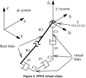
Orthogonal PPPS Virtual Chain (Cartesian System)
A virtual chain useful to describe movements in three-dimensional space is the PPPS orthogonal chain with three prismatic joints whose movements are in the X, Y and Z orthogonal directions and a spherical joint which is instantaneously substituted by three serial orthogonal rotative joints in the X, Y and Z directions, see Fig. 5. The prismatic joints are called px, py and pz, and the rotative joints are called rx, ry and rz.
-system
B
links virtual -system
C
R1
C1
C2
C3
Z
px py
pz
(rx,ry,rz) Y
Z
X
C
C C
S
Real links
R2
X Y
Figure 5. PPPS virtual chain.
The first prismatic joint (px) and the last rotative joint (rz) are attached to the real chain (kinematic chain to be analyzed). Joint px
connects real link R1 with virtual link C1, joint py connects virtual link C1 with virtual link C2, joint pz connects virtual link C2 with virtual link C3 and joint S connects virtual link C3 with real link R2 (see Fig. 5).
Let the twist $px represent the movement of link C1 in relation to
link R1, twist $py represent the movement of link C2 in relation to
link C1, twist $pz represent the movement of link C3 in relation to
link C2, twist $rx+$ry+$rz represent the movement of link R2 in
relation to link C3. Therefore, the movement of real link R2 in
relation to real link R1 may be expressed by
$px+$py+$pz+$rx+$ry+$rz.
Consider the C-reference system (C-system) attached to the virtual link C3 at the spherical joint. Therefore, there is no rotation between the C-system and B-system and the three orthogonal rotative joints are aligned, respectively, with the X, Y and Z axes. So, the normalized screws corresponding to the virtual joints represented in the C-system are
T pz
C T py
C T px
C
T rz
C T ry
C T rx
C
) 1 , 0 , 0 ; 0 , 0 , 0 ( $ˆ , ) 0 , 1 , 0 ; 0 , 0 , 0 ( $ˆ , ) 0 , 0 , 1 ; 0 , 0 , 0 ( $ˆ
) 0 , 0 , 0 ; 1 , 0 , 0 ( $ˆ , ) 0 , 0 , 0 ; 0 , 1 , 0 ( $ˆ , ) 0 , 0 , 0 ; 0 , 0 , 1 ( $ˆ
= =
=
= =
=
(21)
It may be observed that the orthogonal PPPS virtual chain represents the movements in a spatial Cartesian system.
RPPS Virtual Chain (Cylindrical System)
Another useful virtual chain to describe movements in the three-dimensional space is the RPPS kinematic chain composed of a rotative joint (rz) aligned with the Z axis, a prismatic joint (pz) in the
Z axis direction, a prismatic joint (pr) in a direction orthogonal to the Z axis direction (named radial direction) and a spherical joint (S), see Fig. 6. It should be highlighted that when the spherical joint is along the Z axis, the normalized screws corresponding to the rz
and S joints are linearly dependent and the RPPS kinematic chainis in a singularity, and cannot be used as a virtual chain.
C
ZC
-system
B
-system
C
links virtual
links real
R2
R1
P2
P3
P1
r X
α
rz pz pr
X
Y (rn,rt,rb)
Y
(radial)
C(tangential)
(binormal)
S
Z
Figure 6. RPPS virtual chain.
In this virtual chain the first three joints (rz, pz and pr) move into a cylinder. The spherical joint may be instantaneously substituted by three serial orthogonal revolute joints with movements in the normal (rn), tangential (rt) and binormal (rb) cylinder directions.
The joints rz and rb are attached to the real chain: joint rz
connects real link R1 with virtual link P1, joint pz connects virtual link P1 with virtual link P2, joint pr connects virtual link P2 with virtual link P3 and joint S connects virtual link P3 with real link R2 (see Fig. 6).
Let twist $rz represent the movement of link P1 in relation to
link R1, twist $pz represent the movement of link P2 in relation to
link P1, twist $pr represent the movement of link P3 in relation to
link P2, and twist $rn+$rt+$rb represent the movement of link R2 in
relation to link P3. Then, the movement of real link R2 in relation to real link R1 may be expressed by $rz+$pz+$pr+$rn+$rt+$rb.
Consider that the Cˆ -system at the spherical joint is fixed to the
virtual link P3 and that the three orthogonal rotative joints are aligned, respectively, with the
C
normalized screws corresponding to the virtual joints represented in
the Cˆ -system are
(
)
(
)
(
)
(
)
(
)
(
)
Trz C T pz
C T pr
C
T rb
C T rt
C T rn
C
r,0 , 0 ; 1 , 0 , 0 $ˆ ; 1 , 0 , 0 ; 0 , 0 , 0 $ˆ ; 0 , 0 , 1 ; 0 , 0 , 0 $ˆ
0 , 0 , 0 ; 1 , 0 , 0 $ˆ ; 0 , 0 , 0 ; 0 , 1 , 0 $ˆ ; 0 , 0 , 0 ; 0 , 0 , 1 $ˆ
ˆ ˆ
ˆ
ˆ ˆ
ˆ
− = =
=
= =
=
(22)
where r is the ray distance, i.e. the instantaneous distance from the cylindrical axis to the Cˆ -system origin.
It may be observed that the RPPS virtual chain represents a cylindrical coordinate system.
Modified Kinematic Chain
The modified kinematic chain is the closed chain obtained by adding one or more virtual chains to the real chain. The virtual chain selection depends on the information to be obtained or imposed between the real links jointed by the virtual chain.
In this section we describe the modified kinematic chain obtained by adding a virtual chain to a n-link serial manipulator whose movements belong to a d order screw system.
Consider that the manipulator chain has n links (Fig. 7), numbered from zero (link at the base) to n (end-effector). The movement of link (i) in relation to link (i-1) is defined by the kinematic pair Ai, and it is represented by the twist $Ai.
Additionally, $ˆAi represents its corresponding normalized screw.
A
2
1
0
n
A
A n-1
-1 n
A
An 3
2
1
Figure 7. Real n-link manipulator kinematic chain.
Consider that it is necessary to acquire information on or impose movement between the base and the end-effector of the serial manipulator. To achieve this end a suitable virtual chain is added between these two links. A general virtual chain used to modify the open chain is shown in Fig. 8 in thinner lines.
As the manipulator movements belong to a d order screw system, this virtual chain should have d joints with linearly independent normalized screws in order not to change the mobility of the real kinematic chain.
Thus, the virtual chain has d links numbered from (n+1) (link jointed to the base) to (n+d) (link jointed to the end-effector). The relative movement between two adjacent virtual links is defined by the corresponding virtual kinematic pair. The movement of the virtual link (n+1) with respect to the base (link 0) is defined by the kinematic pair B1 and is represented by the twist $B1. The
movement of the virtual link (n+2) with respect to the virtual link (n+1) is given by the kinematic pair B2 and is represented by the
twist 2
$B , and so on.
Serial manipulator pair n-1
d-1
1
B
+ +2
A
-1 2
1
0
Virtual pair 2
1
3
n
n n
n
3 2
d
d n
A
A
A
B
B B
B A
+1
n
Figure 8. Modified (n+d)-link manipulator kinematic chains.
In general, each virtual kinematic pair has only one degree of freedom (f=1). If a pair of the virtual chain has more degrees of freedom (f >1), it could be instantaneously substituted by f serial virtual pairs with one degree of freedom (e.g. spherical pair).
Adding this virtual chain to the manipulator converts the real open chain in a modified closed kinematic chain with (n+d) links.
The kinematic pairs of this modified chain may be divided into actuated (primary) pairs and passive (secondary) pairs like parallel manipulators.
For a serial manipulator in the 3D operational space the order of the screw system is six and the virtual chain has six virtual pairs. These six pairs are represented by six mutually independent twists.
The constraint equation for the modified kinematic chain is obtained by applying the Kirchhoff-Davies circulation law to the modified kinematic chain, considering the circuit direction indicated in Fig. 8, and is given by
0
= − − − − + +
+ A An B B(d-) Bd
A $ $ $ $ $
$
1 1
2
1 (23)
Notice that virtual twists are negative because they represent the velocity of the base in relation to the end-effector, in the opposite direction of the circuit, while the real twists represent the velocity of the end-effector in relation to the base.
The network matrix results in:
[
A A An B B(d-) Bd]
ˆ ˆ ˆ ˆ ˆ ˆ
N=$1$2 $ −$1 −$ 1 −$ (24)
and the velocity magnitude vector is
[
ΨAΨA ΨAnΨB ΨB(d-)ΨBd]
=Ψ 1 2 1 1 (25)
The network matrix (24) and the velocity magnitude vector (25) define the modified kinematic chain constraint equation which allows the calculation of the differential kinematics as is described below.
Differential Kinematics Using Virtual Chains
Differential Kinematics using virtual chains relates the link movements of a kinematic chain applying the Davies method to a virtually modified kinematic chain. Due to the freedom to select the primary kinematic pairs, it is possible to solve different kinematic problems, employing the same method.
kinematics consider the velocity of the end-effector in relation to the base. For this purpose, we add a virtual chain between the base and the end-effector of the serial manipulator as shown in Fig. 8.
Direct Kinematics.
In direct kinematics the objective is to determine the velocity of the end-effector in the operational space as a function of the velocities of the actuated kinematic pairs in the joint space.
To this end the magnitudes of the real kinematic pairs (joint space) are selected as the primary vector components (Ψ p
) and the
magnitudes of the virtual kinematic pairs (operational space) are selected as the secondary vector components (Ψ s
). Thus, Eq.(19) becomes
[
] [
]
− − − − =
−
n n d
)
(d-d )
(d-A A A
A A A B B B
B B
B
Ψ
Ψ
Ψ
$ˆ $ˆ $ˆ $ˆ $ˆ $ˆ
Ψ
Ψ
Ψ
2 1
2 1 1
1 1
1
1
(26)
This highlights that using the virtual kinematic chain concept the Davies method should be extended to calculate the direct differential kinematics of serial manipulators.
Inverse Kinematics.
The inverse kinematics maps end-effector velocities (operational space) into joint velocities (joint space).
To solve the inverse kinematics we select the components of the vector Ψ p
as the magnitudes of the virtual kinematic pairs
(operational space) and the components of the vector Ψ s as the magnitudes of the real kinematic pairs (joint space) of the modified kinematic chain, then Eq.(19) results in
[
] [
]
− − − −
=
−
d ) (d-d ) (d-n
n B
B B
B B B A A A
A A A
Ψ
Ψ
Ψ
$ˆ $ˆ $ˆ $ˆ $ˆ $ˆ
Ψ
Ψ
Ψ
1 1
1 1 2
1 2 1
1
(27)
It could be remarked that, using the virtual kinematic chain concept integrated with the Davies method, the direct and inverse differential kinematics of serial manipulators may be obtained employing the same method, simply by selecting the primary and secondary kinematic pairs according to the desired result.
In the following, the method presented is applied to an industrial robot manipulator.
Differential Kinematics of the PUMA Robot
The direct and inverse differential kinematics of the PUMA robot, considering a Cartesian and a cylindrical operational space, is presented in this section in order to illustrate the approach presented.
The PUMA robot and its variants have widespread use as industrial robots. It is also one of the most studied configurations found in research papers on Robotics. For these reasons, this robot was chosen as an example of differential kinematics using the virtual chains proposed in this work.
The PUMA robot is a serial manipulator with six degrees of freedom. All joints are rotative kinematic pairs. The last three joint axes intersect at a single point forming a so-called spherical wrist.
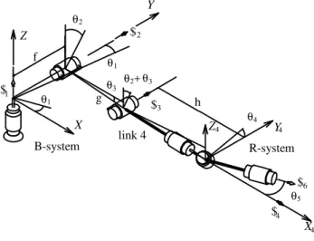
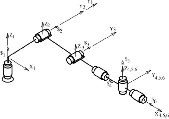
In Fig. 9, θ i
(i=1,…, 6) are the position angles at the rotary joints. The twists $i corresponding to joint movements are aligned
with the joint axes and are shown in the figures as conical arrows.
$4
θ1 2
$
R-system link 4
h
θ θ
θ
θ
$
$
θ
3 2+θ3 3 2
4
5 6
X Y Z
g f
$1
Z
B-system
θ1
Y
4 4
4
X
Figure 9. The Puma robot.
In this paper the PUMA robot differential kinematics is described using screws to represent the movement of the kinematic pairs. The reference frame in which the screws are expressed could be suitably chosen in order to get screws with simple components.
To this end several authors (Hunt, 1987; Martins and Guenther, 2003) use a system fixed to link 4 (X4,Y4,Z4 ) at the center of the
spherical wrist to describe the screws corresponding to the kinematic pairs of the manipulator.
In this work, the reference system fixed to link 1 (base) is named the B-system and the reference system fixed to link 4 is named the R-system, see Fig. 9. The normalized screws of the PUMA robot, represented in the R-system, see Appendix A for details, are (Hunt, 1987)
(
)
(
)
(
)
(
)
(
)
TR
T R
T R
T R
T R
T R
s s s c c
c s
x s
s x c c s
0 , 0 , 0 ; , , $ˆ
) 0 , 0 , 0 ; , , 0 ( $ˆ
0 , 0 , 0 ; 0 , 0 , 1 $ˆ
h , 0 , 0 ; 0 , 1 , 0 $ˆ
, 0 , g ; 0 , 1 , 0 $ˆ
f , , f ; , 0 , $ˆ
5 4 5 4 5 6
4 4 5 4 3
14 23 2
23 14 23 23 23 1
= − = =
− =
′ =
− − −
=
(28)
where, si=sin(θ i); s
ik=sin(θ
i+ θ
k); ci=cos(θ
i); cik=cos(θ
i+ θ
k); etc... 23
2 14 gc hc
x = + ; x14′ =−
(
gc3+h)
; and f, g and h are the distances shown in Fig. 9.Cartesian Operational Space
The Cartesian operational space corresponds to a screw system with d=6. To obtain the differential kinematics in the Cartesian operational space, we chose the PPPS virtual chain presented in Fig. 5 to be added between the base and the end-effector.
$
rx$
ry$
rz(
,
,
)
$
1Circuit
$
2$
3$
4$
5$
6-system
B
-system
$
px$
$
py pz
Z
Y
X
X
Y
Z
C
link of -system
C
Figure 10. Schematic of modified kinematic chain for Puma robot in Cartesian operational space.
According to the Kirchhoff-Davies circulation law the network matrix N of this closed kinematic chain is
[
rx ry rz px py pz]
N=$ˆ1 $ˆ2 $ˆ3 $ˆ4 $ˆ5 $ˆ6−$ˆ −$ˆ −$ˆ −$ˆ −$ˆ −$ˆ (29)
where all the normalized screws are represented in the same coordinate system and the normalized screw signs depend on the circuit direction shown in Fig. 10. The corresponding velocity magnitude vector is
[
rx ry rz px py pz]
TΨ
Ψ
Ψ
Ψ
Ψ
Ψ
Ψ
Ψ
Ψ
Ψ
Ψ
Ψ
Ψ
6 5 4 3 2 1
= (30)
Direct Kinematics in the Cartesian Operational Space
The direct kinematics is obtained by calculating the virtual chain twist magnitudes, which are chosen as the secondary magnitude vector components, i.e.,
[
]
Tpz py px rz ry rx s
Ψ
Ψ
Ψ
Ψ
Ψ
Ψ
Ψ
= (31)
Consequently, the network secondary sub-matrix is given by
Ns=
[
−$ˆrx−$ˆry−$ˆrz−$ˆpx−$ˆpy−$ˆpz]
(32)The primary magnitude vector has the input as components, i.e., the magnitudes of the actuated pairs:
[
]
Tp 1 2 3 4 5 6
Ψ
Ψ
Ψ
Ψ
Ψ
Ψ
Ψ
= (33)
Therefore, the network primary sub-matrix is
Np=
[
$ˆ1$ˆ2$ˆ3$ˆ4$ˆ5$ˆ6]
(34)The secondary magnitude vector is calculated using Eq.(19). In order to simplify the inversion of matrix Ns we choose the C-system
to represent the normalized screws and, thus, Eq.(19) is given by
Ψ s CNs CNpΨ p
1 −
=− (35)
From Eq.(21) it is observed that Ns I
C =− , where
I is the (6×6) identity matrix and employing Eq.(8)
p R R C p
CN = T N (36)
where from Eq.(28)
− ′ − −
− −
=
0 0 0
0 0 0 0 0
0 0 0 0
0 0 0
0 1 1 0
0 1 0 0
14 23 14
23 23
5 4 4 23
5 4 4
5 23
h x fs x
gs fc
s s c c
s c s
c s
Np
R (37)
Thus, the direct kinematics (Eq.(35)) is given by
p p R R C
s T N Ψ
Ψ = (38)
where C
TR is the transformation matrix of screw coordinates
calculated using the rotation matrix C
RR and the position vector CpR
(see Eq.(9)).
There is no rotation between the C-system and the B-system so the C-system is always parallel to the B-system and thus, we have,
R B R C
R
R = (39)
The matrix C
RR is obtained through a matrix product, see (Hunt,
1987) for details, as
− − =
23 23
23 1 1 23 1
23 1 1 23 1
0 c
s s s c c s
s c s c c RR C
(40)
Taking into account that the movements of the spherical wrist do not affect the end-effector translation, the R-system origin may represent the position of the PUMA end-effector. The C-system origin and the R-system origin may then be considered coincident. So the vector C
pR is null.
Therefore, using Eq.(9), the transformation matrix of screws coordinates may be expressed by
[ ]
[ ]
[ ]
[ ]
=
R C R C R C
R R T
0
0 (41)
where
[ ]
0 is the (3 x3 ) zero matrix.Equation (38) establishes the relation between the real joint velocity magnitudes Ψ p
(Ψ 1 ,…,Ψ 6
) and the virtual joint velocity
magnitudes Ψ s (Ψ rx
,…,Ψ pz) which, considering the special configuration of the virtual chain, represent the Cartesian velocity of the end-effector with respect to the base represented in the C -system. The former three components of the velocity state (Ψ rx
,Ψ ry,
rz
Ψ
) are the angular velocities of the end-effector with
respect to the base, represented in the C-system, and the latter three components (Ψ px
,Ψ py ,Ψ pz
) are the linear velocities of a point on
[
]
Tpz py px rz ry rx EE C
Ψ
Ψ
Ψ
Ψ
Ψ
Ψ
$ = (42)
Inverse Kinematics in the Cartesian Operational Space
The inverse kinematics is obtained by calculating the real chain twist magnitudes which, in this case, are chosen as the secondary magnitude vector components,
[
]
Ts 1 2 3 4 5 6
Ψ
Ψ
Ψ
Ψ
Ψ
Ψ
Ψ
= (43)
Accordingly, the network secondary sub-matrix is
[
$ˆ1$ˆ2$ˆ3$ˆ4$ˆ5$ˆ6]
=
s
N (44)
The primary magnitude vector has the input as components, i.e., the magnitudes of the virtual pairs:
Ψ p
[
Ψ rxΨ ryΨ rzΨ pxΨ pyΨ pz]
T= (45)
Thus, the network primary sub-matrix is given by
Np=
[
−$ˆrx−$ˆry−$ˆrz−$ˆpx−$ˆpy−$ˆpz]
(46)The secondary magnitude vector is calculated using Eq.(19), which, aiming at simplifying the inversion of the network secondary sub-matrix (Ns,), R-system is represented as
p p R s R
s N N
Ψ
Ψ −1
=− (47)
where, using Eq.(28),
− ′ − −
− −
=
0 0 0
0 0 0 0 0
0 0 0 0
0 0 0
0 1 1 0
0 1 0 0
14 23 14
23 23
5 4 4 23
5 4 4
5 23
h x fs x
gs fc
s s c c
s c s
c s
Ns
R (48)
and employing Eq.(8)
p C C R p R
N T
N = (49)
where from Eq.(21) it could be observed that CN p=-I.
Thus, replacing Eq.(48) and Eq.(49) into Eq.(47), the inverse kinematics becomes
p C R s R
s N T
Ψ
Ψ −1
= (50)
Note that the transformation of the screw matrix, according to Eq.(11) and Eq.(41) may be written as
[ ]
[ ]
[ ]
[ ]
=
= −
T R C T R C R C C R
R R T
T
0 0
1 (51)
Equation (50) establishes the inverse differential kinematics of the PUMA robot where the end-effector velocity is given in the Cartesian system described by the virtual chain.
Matrix R
Nsin Eq.(50) is the Jacobian of the PUMA manipulator
when it is calculated throughout the screw theory (Hunt, 1987), i.e.
the screw based Jacobian. The method presented in this paper, like the screw based Jacobian method, allows the selection of a suitable coordinate system (R-system) aiming at obtaining a sparser Jacobian matrix.
Cylindrical Operational Space
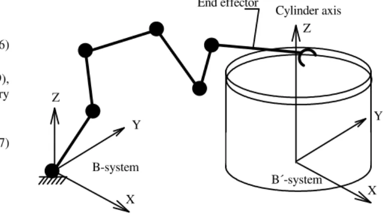
For certain tasks, the description of the movements in operational spaces other than the Cartesian could be useful. For instance to represent a radial or tangential velocity of the end-effector to weld a pipe, the cylindrical operational space may be more suitable than the Cartesian space.
In order to illustrate the flexibility of the approach presented in this paper, the direct and inverse differential kinematics of the PUMA robot using a general cylindrical operational space is presented below.
Consider a robot welding around a pipe whose axis coincides with the Z axis of the B´-system shown in Fig. 11.
Z
Y
X
End effector
B-system
Cylinder axis
Y
X B´-system
Z
Figure 11. Schematic of Puma robot welding a pipe.
The cylindrical operational space corresponds to a screw system in which d=6. To obtain the differential kinematics in the cylindrical operational space, we chose the virtual chain RPPS presented in Fig. 6 to be added between the base and the end-effector.
For this case the modified kinematic chain is shown in Fig. 12.
$2
$3
$4
$5
$6
$1
Circuit
$rz $pz pr $ , ($rn$rt,$rb) End effector
Applying the Kirchhoff-Davies circulation law, regarding the circuit direction indicated in Fig. 12, the network matrix N results in
[
rn rt rb pr pz rz]
N= $ˆ1$ˆ2$ˆ3$ˆ4$ˆ5$ˆ6−$ˆ −$ˆ −$ˆ −$ˆ −$ˆ −$ˆ (52)
and the corresponding velocity magnitudes vector is
[
]
Trz pz pr rb rt rn
Ψ
Ψ
Ψ
Ψ
Ψ
Ψ
Ψ
Ψ
Ψ
Ψ
Ψ
Ψ
Ψ
6 5 4 3 2 1
= (53)
Direct Kinematics in the Cylindrical Operational Space
The direct kinematics is obtained by calculating the virtual chain screw magnitudes which are chosen as the secondary magnitude vector components,
[
]
Trz pz px rb rt rn s
Ψ
Ψ
Ψ
Ψ
Ψ
Ψ
Ψ
= (54)
Consequently, the network secondary sub-matrix is given by
Ns=
[
−$ˆrn−$ˆrt−$ˆrb−$ˆpx−$ˆpz−$ˆrz]
(55)The primary magnitude vector has the input as components, i.e., the magnitudes of the actuated pairs:
[
]
Tp 1 2 3 4 5 6
Ψ
Ψ
Ψ
Ψ
Ψ
Ψ
Ψ
= (56)
Therefore, the network primary sub-matrix is
Np=
[
$ˆ1$ˆ2$ˆ3$ˆ4$ˆ5$ˆ6]
(57)The secondary magnitude vector is calculated using the constraint equation shown in Eq.(19). To simplify the inversion of
matrix Ns we chose the Cˆ -system to represent the normalized
screws and thus Eq.(19) is given by
p p C s C
s N N Ψ
Ψ
ˆ 1 ˆ −
=− (58)
where, using Eq.(22),
− −
− − − −
=
0 1 0 0 0 0
0 0 0 0 0
0 0 1 0 0 0
1 0 0 1 0 0
0 0 0 0 1 0
0 0 0 0 0 1
ˆ
r Ns
C (59)
and employing Eq.(8)
p R R C p C
N T
N ˆ
ˆ
= (60)
The screw coordinates matrix transformationC R
T ˆ
is calculated
using the rotation matrix CˆRR and the position vector CˆpR.
Considering that the origins of the Cˆ -system and R-system
coincide, the vector CˆpR is null. The rotation matrix R CˆR may be
obtained by the matrix product
R B B C R C
R R
R ˆ
ˆ
= (61)
where B
RR is described in Eq.(40-41) and
− =
1 0 0
0 0
) ( ) (
) ( ) ( ˆ
rz rz
rz rz
B C
c s
s c
R (62)
where c(rz) and s(rz) represent the cosine and sine, respectively, of the
instantaneous angular position θ rz
of the virtual rotative pair $rz. It
could be observed that the angleθ rz
is null when the Cˆ -system and
the B-system are parallel.
Therefore, the transformation matrix CˆTR is given by
[
]
[ ]
[ ]
[
]
=
R B B C R B B C R C
R R R R
T ˆ
ˆ ˆ
0
0
(63)
The calculation of the direct kinematics is obtained using Eq.(58)
p P R R C s C
s N T N Ψ
Ψ
ˆ 1 ˆ −
=− (64)
Equation (64) describes the relation between the real joint velocity magnitudes p
Ψ
(Ψ 1,…, 6
Ψ ) and the virtual joint velocity magnitudes Ψ s (
rx
Ψ ,…,
az
Ψ ) which, considering the special configuration of the virtual chain, represent the cylindrical velocity of the end-effector with respect to the base represented in the Cˆ
-system. The former three terms (Ψ rn,
rt
Ψ ,
rb
Ψ ) of the end-effector velocity state represent the angular velocity (normal, tangential and binormal) of the end-effector with respect to the base, represented
in the Cˆ -system. The latter three (Ψ px,
pz
Ψ ,
rz
Ψ .) indicate, respectively, the radial linear velocity Ψ px
, the axis linear velocity
pz
Ψ
and the azimuthal angular velocity Ψ rzof a point on the
end-effector, instantaneously at the Cˆ -system origin, with respect to the
base, represented at the Cˆ -system.
Inverse Kinematics in the Cylindrical Operational Space
The inverse kinematics is obtained by calculating the real chain screw magnitudes which are the secondary magnitude vector components, i.e.,
[
]
Ts 1 2 3 4 5 6
Ψ
Ψ
Ψ
Ψ
Ψ
Ψ
Ψ
= (65)
Then, the network secondary sub-matrix is
Ns=
[
$ˆ1$ˆ2$ˆ3$ˆ4$ˆ5$ˆ6]
(66)The primary magnitude vector contains the magnitudes of the virtual pairs:
[
]
Trz pz pr rb rt rn p
Ψ
Ψ
Ψ
Ψ
Ψ
Ψ
Ψ
= (67)
[
rn rt rb pr pz rz]
p
N =−$ˆ −$ˆ −$ˆ −$ˆ −$ˆ −$ˆ (68)
The secondary magnitude vector is calculated using the constraint equation (Eq.(19)), which, aiming to simplify the inversion of the matrix, is represented in the R-system, as shown in Eq.(47), here repeated
p p R s R
s N N
Ψ
Ψ −1
=− (69)
and employing Eq.(8)
C p
C R p R
N T
N = ˆˆ (70)
where the transformation of the screw coordinate matrix, using Eq.(11), is
[
]
[ ]
[ ]
[
]
=
= −
T R B B C T R B B C
R C C R
R R R R T
T ˆ
ˆ 1 ˆ ˆ
0
0 (71)
So, the inverse kinematics, using Eq.(69), is given by
p p C C R s R
s N T N Ψ
Ψ
ˆ ˆ 1 −
=− (72)
It should be remarked that the inverse differential kinematics is obtained by inverting the matrix corresponding to the manipulator joint screws represented in the R-system, the same matrix is inverted to obtain the inverse kinematics in the Cartesian operational space.
Similarly, by adding a suitable virtual chain, between the base and end-effector, it is to possible calculate the inverse differential kinematics based on the end-effector velocity given in a spherical coordinate system.
This example shows that the proposed method allows the determination of the inverse differential kinematics in a coordinate system (Cartesian, cylindrical etc.) suitable for the end-effector task. This is not so evident achieved using conventional methods (e.g.
Denavit-Hartemberg based method and screw based method).
Conclusions
This paper presents a simple, systematic and unified approach to obtain the differential kinematics of serial manipulators using the screw representation.
By introducing a virtual chain concept in order to close open kinematic chains it is shown that the differential kinematics of serial manipulators can be calculated using the Davies method, a simple and systematic way to relate the joint velocities in closed kinematic chains.
The proposed approach results unified because the direct and the inverse kinematics are obtained in a similar way, by selecting variables according the desired result.
Furthermore, the approach allows the determination of the inverse differential kinematics in a coordinate system (Cartesian, cylindrical, etc.) suitable for the end-effector task, which could be very useful, and this is not trivially achieved using conventional methods.
Like the screw based Jacobian method, the presented approach allows the selection of a suitable coordinate system aiming at a sparser Jacobian matrix.
Acknowledgments
This work was partially supported by `Fundação Coordenação de Aperfeiçoamento de Pessoal de Nível Superior (CAPES)', Brazil, and by `Conselho Nacional de Desenvolvimento Científico e Tecnológico (CNPq)´, Brazil.
Appendix A
In this appendix a method to calculate the normalized screws correponding to the joint movements of the PUMA robot is presented.
Aiming to find the screws corresponding to the PUMA joints, we first define a reference (home) configuration for the manipulator and a coordinate system fixed to each link, namely 1,2, ... and 6. Although the reference position can be chosen arbitrarily, it is usually chosen at a location where, if possible, all the joint axes are parallel or orthogonal. The reference configuration for PUMA and the coordinate systems 1,2,... and 6 fixed to the respective links are showed in Fig. A1 where all the joint angles (θ i
) are null and the coordinate systems are parallel.
Z Z
$1 Z
Z
$5 $2
$3
$6 $4
Y2
Y 1
2
4,5,6
4,5,6
4,5,6 X1
3
3
Y
X Y1
Figure A1. The Puma robot reference configuration.
According to Eq.(3) the normalized screws of joints 1,2,.. and 6 expressed, respectively, at the coordinate system 1,2,… and 6 are easily identified as
(
)
(
)
(
)
(
)
(
)
(
)
TT T T T T
0 , 0 , 0 ; 0 , 0 , 1 $ˆ
0 , 0 , 0 ; 1 , 0 , 0 $ˆ
0 , 0 , 0 ; 0 , 0 , 1 $ˆ
0 , 0 , 0 ; 0 , 1 , 0 $ˆ
0 , 0 , 0 ; 0 , 1 , 0 $ˆ
0 , 0 , 0 ; 1 , 0 , 0 $ˆ
6 6
5 5
4 4
3 3
2 2
1 1
= = = = = =
(A1)
where the subindex represents the joint and the superindex represents the coordinate system where the normalized screws are described.
Considering the coordinate systems of Fig. A1, the rotation matrices i i
R 1
− and the vectors i i
p 1
− between adjacent coordinate