Todos os direitos reservados.
É proibida a reprodução parcial ou integral do conteúdo
deste documento por qualquer meio de distribuição, digital ou
impresso, sem a expressa autorização do
REAP ou de seu autor.
Labor Earnings Dynamics in Post-Stabilization
Brazil
Amanda Cappellazzo Arabage
André Portela Souza
Labor Earnings Dynamics in Post-Stabilization Brazil
Amanda Cappellazzo Arabage
André Portela Souza
Amanda Cappellazzo Arabage1
R. Itapeva, 286. Sao Paulo, SP, Brazil, 01332-000
Sao Paulo School of Economics (EESP/FGV)
Center for Applied Microeconomic Studies (C-Micro/EESP/FGV)
André Portela Souza
R. Itapeva, 474/1205. Sao Paulo, SP, Brazil, 01332-000
Sao Paulo School of Economics (EESP/FGV)
Labor Earnings Dynamics in Post-Stabilization Brazil
✩May 12, 2015
Amanda Cappellazzo Arabage1
R. Itapeva, 286. Sao Paulo, SP, Brazil, 01332-000
Sao Paulo School of Economics (EESP/FGV)
Center for Applied Microeconomic Studies (C-Micro/EESP/FGV)
Andr´e Portela Souza2,∗
R. Itapeva, 474/1205. Sao Paulo, SP, Brazil, 01332-000
Sao Paulo School of Economics (EESP/FGV)
Center for Applied Microeconomic Studies (C-Micro/EESP/FGV)
Abstract
This paper analyzes both the levels and evolution of wage inequality in the Brazilian formal labor market using administrative data from the Brazilian Ministry of Labor (RAIS) from 1994 to 2009. After the covariance structure of the log of real weekly wages is estimated and the variance of the log of real weekly wages is decomposed into its permanent and transitory components, we verify that nearly 60% of the inequality within age and education groups is explained by the permanent component, i.e., by time-invariant individual productive charac-teristics. During this period, wage inequality decreased by 29%. In the first years immediately after the macroeconomic stabilization (1994−1997), this decrease is explained entirely by
re-ductions in the transitory component, suggesting that the end of the macroeconomic instability was a relevant factor in reducing inequality. In the second sub-period (1998−2009), the
de-crease is mostly explained by reductions in the permanent component. Finally, we show that education and age account for a sizable share of the permanent component (54% on average).
Keywords: Earnings dynamics, wage inequality, formal labor market, variance decomposition
JEL:J3, J6, O5
✩The authors would like to thank Sao Paulo School of Economics (EESP/FGV) and Con-selho Nacional de Desenvolvimento Cientfico e Tecnolgico (CNPq) for financial support.
∗Corresponding author.
1
amanda.arabage@fgv.br
2
1. Introduction
It has been well documented that Latin American countries have experienced
decreased income inequality over the most recent two decades and that these
decreases are mostly associated with decreased inequalities in labor earnings
(e.g., Lopez-Calva and Lustig (2010) [31]; Azevedo et al. (2013) [2]). However,
the underlying forces behind these trends remain the subject of debate. Some
authors argue that such trends are mainly explained by structural changes in
the economic fundamentals of these countries. For instance, relying on studies
of Argentina, Brazil, and Mexico, Lustig et al. (2013) [33] explain the decrease in inequality by the decrease in the observed skill premia. Manacorda et al.
(2010) [35] also find a decline in the skill premia and argue that it is largely
explained by the sharp rise in the supply of secondary-level educated workers
relative to primary-level educated workers in the 1980s and 1990s. Additionally,
for selected countries in Latin America, there is evidence that openness to trade
reduced wage differentials in the 1990s (e.g., Gonzaga et al. (2006) [22] and
Ferreira et al. (2007) [18] for Brazil and Robertson (2004 [44], 2007 [45]) for
Mexico). However, other authors argue that the decrease in inequality may be
attributable to more transient factors. For instance, Gasparini et al. (2011) [21]
argue that the increase in the supply of more educated workers cannot account for the decrease in inequality. Other factors including changes in terms of trade
(e.g., the commodities boom) and changes in trade and industrial policies are
likely to be more important. The authors also suggest the possibility that skill
mismatches reduce the productivity of highly educated workers. Additionally,
Gasparini et al. (2009) [20] posit the hypothesis that the observed
compres-sions in wage distributions may be associated with realignments after the strong
shocks of the 1990s in the region.
We aim to shed some light on this debate by examining the relative
impor-tance of these two groups of factors in a unified framework. Specifically, we
country Brazil in the 1990s and 2000s. We rely on a large body of literature
that discusses the causes of changes in wage inequalities in the United States
and other developed countries. In particular, there is a branch of this literature
that addresses this issue by quantifying the relative importance of transitory and
permanent shocks over time. By examining the relative importance of each, it is possible to understand the underlying factors that might explain the evolution
of inequality, which is helpful for understanding the functioning of the labor
market and for designing appropriate public policies3 . This literature is well
suited to help clarify the debate on the underlying causes of the decreases in
wage inequality in the Latin American region.
In contrast to developed countries, Latin American countries (including
Brazil) have recently experienced decreases in inequalities in their labor
earn-ings. As we document below, the decreases in wage inequality also occur within
groups by education level and age (at least in the country we analyze). To the
best of our knowledge, there is no systematic data and analysis available re-garding the evolution of unobserved skills and their returns in the region or on
the relative importance of transitory and permanent shocks in explaining the
decline in the region’s wage inequality observed during the post-stabilization
period. This paper aims to fill this gap by exploring a unique panel dataset
from Brazil that covers an extended period of time.
The permanent wage component relates to workers’ productivity
charac-teristics (such as human capital), whereas the transitory component is
associ-ated with noise caused by economic instability. In other words, the permanent
3
component is associated with individuals’ wage profiles during their lifetimes,
whereas the transitory component represents stochastic fluctuations. A
down-trend or updown-trend in inequality may be explained by different factors. A decrease
in inequality resulting mainly from a decrease in the permanent component is
associated with a mobile labor market in which workers are able to change posi-tions in wage distribution during their lifetimes. Individuals with lower lifetime
earnings have relatively larger increases in their earnings. A change in demand
in favor of less skilled workers would cause a shift in wage distribution; thus, the
position occupied by each worker would change, which would lead to a decrease
in the variance of the permanent component and, ultimately, in the variance of
inequality. This result, for example, would be consistent with openness to trade
where less-skilled workers are relatively more abundant.
By contrast, a decrease in inequality resulting from a decrease in the
tran-sitory component is related to lower mobility. In this case, changes occur in
wage distribution, but the positions occupied by workers remain unchanged; there are no systematic changes in their lifetime earnings. Some possible causes
for changes in the transitory component are macroeconomic shocks that affect
workers differently, changes in competition and weaker worker-firm attachment
(Haider (2001) [25]), changes in regulations or in union activities and even
changes in the demand for temporary jobs and for self-employment (Moffitt and
Gottschalk (2012) [40]).
Understanding which component is responsible for the variation in inequality
is important both to check the impact on social welfare (given that permanent
and transitory shocks have different effects) and to design public policies that
are appropriate for the proper functioning of the labor market. If the permanent component is predominant, policies oriented toward enhancing worker education
and qualifications and toward better matching between workers and firms are
more appropriate. However, if the transitory component is stronger, policies
should be adopted that mitigate the effects of any negative shocks workers may
suffer in the labor market. Wage instability particularly when it results from
consumption. Because individuals’ welfare depends on their capacity to smooth
consumption over their lifetimes (Friedman (1957) [19]), transitory shocks are
more easily absorbed than permanent shocks and are therefore associated with
reduced social welfare loss and reduced impact on inequality.
Most of the previous literature has sought to explain the increases in wage inequality that have been observed in developed countries, such as the United
States (Lillard and Willis (1978) [29], MaCurdy (1982) [34], Baker (1997) [3],
Haider (2001) [25], Moffitt and Gottschalk (2011) [39], Hryshko (2012) [28],
Moffitt and Gottschalk (2012) [40] and Lochner and Shin (2014) [30]), Canada
(Baker and Solon (2003) [4] and Beaudry and Green (2000) [6]), the United
Kingdom (Ramos (2003) [42] and Dickens (2000) [15]), Italy (Cappellari (2000)
[10]) and Norway (Blundell, Graber and Mogstad (2014) [7]).
To the best of our knowledge, there is no such decomposition exercise for a
developing country and finding evidence of transitory and permanent
inequal-ities for a developing country is interesting in and of itself. Additionally, we have a rare opportunity to exploit a long-period longitudinal dataset from a
representative country in Latin America to investigate possible explanations for
the decreases in wage inequality experienced throughout the region in recent
decades. This paper assesses the changes in formal wage inequality in Brazil
between 1994 and 2009 using variance decomposition, as referenced in the labor
economics literature. After the covariance structure of the log of real weekly
wages is estimated and the variance of the log of real weekly wages is
decom-posed into permanent and transitory components, we verify that nearly 60% of
the inequality within age and education groups is explained by the permanent
component, i.e., by time-invariant individual productive characteristics. We also show that education accounts for a sizable share of this component (54%, on
average).
The overall wage inequality decreased over the 1994−2009 period. This
wage inequality decrease is also observed within formal and informal sectors.
In the years immediately following the stabilization of the Brazilian economy
the decline in the transitory component of wage inequality. By contrast, in
the second sub-period (1998−2009), the decrease in formal wage inequality is
mostly explained by the decrease in the permanent component of wage
inequal-ity. These findings suggest, first, that (the end of) economic instability is an
important element in the explanation of the decrease in inequality, and its ef-fects can be immediately sensed in the labor market. Second, changes in the
fundamentals also have an important role in explaining the decrease in
inequal-ity following economic stabilization. Notably, because we use wage inequalinequal-ity
within education and age groups, the changes in the fundamentals are associated
with factors beyond education and demographic composition changes.
The paper is organized in seven sections, including this introduction. The
second section presents stylized facts about the economic performance and
evo-lution of wage inequality in Brazil over recent decades. The third section
presents the empirical models and estimation method. The fourth section
de-scribes the dataset and the sample used. The fifth section presents the results, and the sixth section presents a more detailed discussion of certain results. The
seventh section concludes.
2. Economic Instability and Wage Inequality in Brazil
Latin American countries, including Brazil, experienced strong
macroeco-nomic instability in the 1980s and 1990s. This period included a sequence of
negative economic shocks that led to high inflation and volatile growth.
Af-ter four failed attempts to control inflation, the Brazilian government finally
launched a successful stabilization plan, the Real Plan, in 1994. Concurrently,
Brazil and the region implemented market structural reforms such as
imple-menting economic openness to trade, government reforms, privatization,
dereg-ulation and liberalizations in the financial sector throughout the 1990s (see, e.g.,
Edwards (1995) [17] and Lora (2012) [32]).
launched based on a pegged exchange rate in mid-1994. A new currency was
established (the Real), and inflation was finally controlled. From 2,477% a year
in 1993, the inflation rate decreased to a single-digit rate in 1996 and remained
near the single-digit range during most of the subsequent period. Economic
growth was volatile in the 1990s, ranging from 4% a year to no growth in the second part of the decade. In the 2000s, Brazil experienced better economic
performance with higher growth rates (an average of approximately 4%
annu-ally, with the exception of 2009, the year of the global financial crisis). Adult
unemployment rose after the price stabilization from approximately 5% to 10%
in 2003 but decreased to approximately 7−8% by the end of the first decade of
the 2000s.
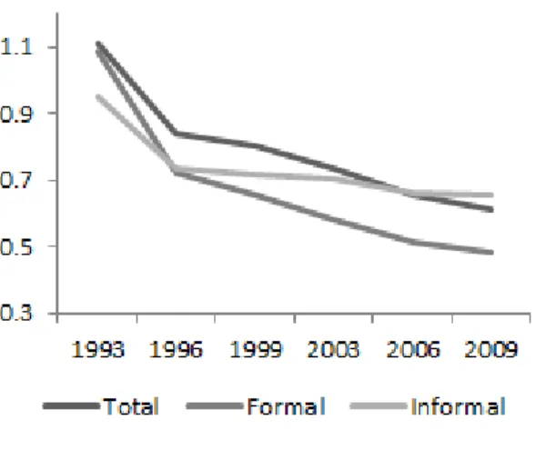
Using the Brazilian National Household Survey (PNAD/IBGE) for selected
years, we note that wage inequality decreased throughout the period for all
waged workers and for both formal and informal waged workers separately. The
average proportion of formal waged workers is 71% and the standard deviation is 0.024. Figure 1 presents the evolution of the variance of the log of real wages,
and Figure 2 presents the variance of the residual of the regression of the log of
real wages on age and education dummies.
We note that wage inequality decreased between 1993 and 2009. This pattern
is observed whether considering the variance of the unconditional log of real
wages or the variance of residuals. Figure 1 shows that there was a decrease in
unconditional wage inequality during the period. Figure 2 shows that there was
a decrease in within-group (age and education level) wage inequality during the
period.
These trends are not sensitive to the inequality measure used; we found the
4
Figure 1: Variance of the log of real wage. Inequality Measures: Brazil (selected years). Source: Brazilian National Household Survey (PNAD/IBGE).
Figure 2: Variance of residuals. Inequality Measures: Brazil (selected years). Source: Brazil-ian National Household Survey (PNAD/IBGE).
same patterns using the Gini coefficient and the Theil measure. Regardless of
the inequality measure used, there is evidence of a decrease in wage inequality
among both formal waged workers and informal waged workers. Understanding
The changes in the economic environment and in wage inequality may be
linked in a number of ways. On the one hand, the structural changes in the
Brazilian economy in recent decades may have caused permanent shocks in
the labor market. Openness to trade, skilled-biased technological changes, and
demographic and skill composition changes in the workforce may have changed the distribution of skills, occupations and their returns in the market.
On the other hand, alongside the structural changes, the end of economic
instability may have contributed to the decrease in wage inequality by reducing
the frequency of negative transitory shocks. The Brazilian economy experienced
a number of external shocks in the 1990s but enjoyed a positive external
envi-ronment in the 2000s with favorable terms of trade and a commodities boom.
Moreover, before inflation was curbed, Brazilians had been living under high
and volatile inflation for more than a decade. As a result, they had developed
mechanisms to work around inflation, such as indexation mechanisms, specific
financial contracts, and formal and informal labor agreements. When these mechanisms are unevenly distributed across individuals, inflation can
exacer-bate inequality. Indeed, Cysne et al. (2005) [14] show formally that in an
economy in which (i) the higher the inflation the more monetary assets are
substituted by shopping time and (ii) the poor have more restricted access to
financial assets, a positive link can be found between inflation and inequality as
long as the productivity of the interest-bearing assets in the transacting
tech-nology is sufficiently high. In fact, there is evidence from Argentina that people
do take more time to shop during an economic crisis (Mackenzie and
Schar-grodsky (2011) [36]). Additionally, there is evidence from Brazil that inflation
and wage inequality are positively correlated (Cardoso et al. (1995) [11], Bar-ros et al. (2000) [5] and Souza (2002) [46]). Under very low inflation, this
inequality-enhancing mechanism is no longer relevant.
In this paper, we will not examine one or some specific mechanisms directly.
Instead, we will apply an earnings dynamics model that evaluates the relative
importance of the permanent and transitory components associated with wage
3. Models and Estimation Methods
Variance decomposition models decompose covariance into two types of
com-ponents: permanent and transitory. This type of model is commonly used in
studies whose objective is to explain cross-sectional inequality and its
evolu-tion over time. By modeling a labor income funcevolu-tion based on permanent and
transitory components, the variance and covariance of earnings can be analyzed
over time, which allows the importance of each component to be assessed in the
cross-sectional variance as well as in their changes over time. To avoid
partic-ipation self-selection bias issues, this study (like most studies) considers only economically active prime-age males.
3.1. The Covariance Structure
Consider the following canonical model5:
yit=µi+vit (1)
whereyit is a measure of individuali’s earnings attand corresponds to the
sum of a time-invariant individual componentµi, which is uncorrelated between
individuals, and of a serially uncorrelated transitory component (white noise),
vit. We also have that:
µi∼iid(µi, σµ2) (2)
vit∼iid(0, σ2v) (3)
Assuming both components are orthogonal, such that Cov(µi, vit) = 0, we
obtain:
5
Cov(yit, yis) =
σ2
µ+σv2 for t=s
σ2
µ for t6=s
(4)
The variance of the permanent component (σ2
µ) represents the effect of
in-dividuals’ characteristics whether observable or not that do not change over
time, fully determining the covariance between different time periods, as the
transitory component corresponds to white noise.
Because this approach has strict constraints on the dynamic structure, a
number of authors have proposed more sophisticated and complex approaches.
The permanent component may be modified by including time-varying factor
models (factor loads), and the transitory component may be treated as a time
series model (ARMA(p, q))6. In matrix notation, we have:
yit=ρ′tµi+vit (5)
a(L)vit=m(L)ǫit (6)
where ρ′
t = (ρ1t, . . . , ρgt) is a 1×g vector of coefficients that may or may
not be known,µ′
i= (µ1, . . . , µg) is a 1×gvector of time invariant disturbances
with:
E(µiµ′j) =
σµ2 if i=j
0 otherwise (7)
andLis a lag operator such that the roots ofm(L) = 0 lie outside the unit
circle by hypothesis, andǫit is white noise with:
E(ǫitǫjt∗) =
σ2
ǫ if i=j andt=t∗
0 otherwise (8)
6
In this case, the covariance matrix is given by:
Ω =E(yityit′ ) =ρσ2µρ′+E(vitv′it) (9)
Depending on the ARMA(p, q) model used for vit, the covariance matrix
changes via E(vitvit′ ). We tested the following different specifications: AR(1),
ARMA(1,1), ARMA(1,2), AR(2), ARMA(2,1) and ARMA(2,2)7. AR(1) was
the specification with the best fit, and this model is described below. Assuming
vitfollows an AR (1) process, we have:
yit=ρtµi+vit (10)
vit=φvit−1+ǫit (11)
where:
µi∼iid( ¯µi, σµ2) (12)
ǫit∼N(0, σǫ2) (13)
E(ǫitǫjt∗) =
σ2
ǫ if i=j andt=t∗
0 otherwise (14)
Cov(µi, vit) = 0 (15)
Including parameterσ2
v−1, which corresponds to the variance of the
transi-tory component (vit) in the period immediately before the initial period, it is
possible to identify the variance ofyit as:
7
V ar(yit) =ρ2tσµ2+φ2(t+1)σ2v−1+
t
X
j=0
φ2(t−j)σ2
ǫ (16)
Additionally, the covariance between periodst andt+sis:
Cov(yit, yit+s) =ρtρt+sσµ2+φ2t+s+2σv2−1+
t
X
j=0
φ2t+s−2jσ2
ǫ (17)
Inequality in the labor market may be decomposed as a whole (by directly
analyzing wages) and/or within age and education groups. To do so, the same
analysis is conducted using the residuals of the regression of the log of wages on
the age and education indicator variables. Because we aim to investigate the
trends in unobserved skills and to control for changes in workers’ demographic
and education compositions within the formal sector, we first present the results
for the residuals of the log of wages. We also performed the same
decomposi-tion for uncondidecomposi-tional wages, and the results, which are presented succinctly in
subsection 6.2 below, are qualitatively similar8.
3.2. Estimation
Using individual panel data on the log of real weekly wages overT periods,
it is possible to calculate observed covariance matrices C, and the covariance
matrix of observed covariance, V9. As shown in the previous subsection, the
elements of the covariance matrix for the log of wages can be modeled in various and distinct ways. Consider any model that depends on a vector of parameters
b(whose size is smaller than T) such thatm=f(b). We can estimateb using
minimum distance methods in which the following expression is minimized:
(m−f(b))′A(m−f(b)) (18)
whereAcorresponds to a positive definite weighting matrix (Dickens (2000)
[15]). Hence,bis chosen to reduce the distance between the observed moments
8
These results are available upon request.
9
m and the theoretical moments predicted by the model f(b) as close to zero
as possible. For the specific case of the AR(1) model with factor loads, the
expression to be minimized is indicated in Appendix B.
Let R−1 be the inverse matrix of R = P V P′, where V is the covariance
matrix of the log of wage covariance, and P = I −F(F′AF)−1F′A, where F=F(b∗) is the Jacobian matrix assessed inb∗ (the estimated value ofb):
F(b∗) =∂f(b) ∂b (b
∗) (19)
Inference is made based on the following statistic, which, under the null
hypothesis thatm=f(b∗) (equivalent to the specification used being correct),
has a chi-squared asymptotic distribution (as demonstrated by Newey (1985)
[41]):
n[(m−f(b∗))′R−(m−f(b∗))]∼χ2
h (20)
where R− corresponds to the generalized inverse10 of matrix R, and h is
the number of degrees of freedom, representing the difference between the size
ofmand the rank of the Jacobian matrix assessed in b∗(F(b∗)). This statistic
may be used to test the general structure of the model and to compare different
methods.
The standard errors of the estimated parameters can be obtained by
calcu-lating the asymptotic variance ofb∗, thus allowing forttests to be conducted for
each of the estimated coefficients. According to Chamberlain (1984) [12], under
some conditions,b∗ converges to the true value ofb and √n(b∗−b) converges
in distribution to N(0,Ω), where Ω = (F′AF)−1F′AV AF(F′AF)−1. We can
treatb∗as if:
b∗∼N(b,Ω/n) (21)
such that the asymptotic variance ofb∗ can be estimated using:
10
AV ar(b∗) = [(F′AF)−1F′AV AF(F′AF)−1]/n (22)
The choice of A determines the type of minimum distance to be estimated.
One alternative would be the optimal minimum distance method, where A =
V−1and whereV−1corresponds to the inverse matrix ofV (covariance matrix
of covariance), thereby minimizing:
(m−f(b))′V−1(m−f(b)) (23)
This method is referred to as optimal because it minimizes the asymptotic
variance ofb∗, reducing it to Ω = (F′V−1F)−1.
Another alternative is the equally weighted minimum distance, whereA=I,
minimizing (m−f(b))′(m−f(b)). In this case, the weight attributed to each
moment is the same. However, because an unbalanced panel is used and different
numbers of observations are thus utilized for each estimated moment, giving
equal weights to different moments may not be appropriate.
Following Haider’s (2001) [25] suggestion, we chooseA= Π−1Π−1, where:
Π = n1
n 0 · · · 0
0 n2
n · · · 0
..
. ... . .. ...
0 0 · · · nL
n (24)
and nl corresponds to the number of observations used to calculate
mo-mentl, andnis the total number of observations. Therefore, a larger weight is
attributed to moments for which there are proportionally more available obser-vations.
4. Data
The decomposition exercise requires the availability of a long period panel
dataset of workers. Brazil has such a dataset. We use data from the Annual
and Employment. Firms that hire workers formally report information about
the wages and occupations of all their workers to the Ministry on an annual
basis11, in addition to individual characteristics such as education, gender and
age. Because each worker has a unique identification number that comes from
registering in the Brazilian Social Integration Program (PIS), it is possible to follow individuals over time as long as they stay in the formal labor market.
The advantage of this panel dataset is that it follows a large number of
work-ers over a relatively long period of time. In particular, it covwork-ers a previous period
of macroeconomic instability that is followed by a period of stability. The
draw-back is that it does not include informal workers. However, decomposing wage
inequality into permanent and transitory components among formal workers in
a developing country is interesting in and of itself, and, more importantly, it
still sheds light on the roles played by economic instability and lifetime earnings
distribution in changing wage inequality in the Latin American region.
There were more than 54 million PIS identification numbers from male indi-viduals in the RAIS administrative database that appeared at least once in the
period between 1994 and 2009. A 5% random sample was chosen from the list
of the PIS identification numbers of all male individuals12. Furthermore, the
sample was restricted to male individuals aged 25 to 64 years old with reported
information regarding at least one valid wage.
We begin in 1994 to minimize measurement error problems. Before 1994,
wages were reported in different currencies. Because of the high inflation,
nomi-nal wages changed monthly or even weekly, and it is not clear that wage changes
were reported to the Ministry correctly. We end in 2009 because it is the last
year with available information to us.
11
All formal employers in Brazil must provide information on their employees to the Ministry of Labor and Employment (MTE), pursuant to Executive Order n. 76.9000 of September 23, 1975.
12
Table 1 reports the number of available observations in each stage of this
sample selection process.
Stage Number of Individuals
(Male)
Appeared at least once between 1994 and 2009 54,344,896
Sample of 5% 2,717,245
Sample of 5%, 25 to 64 years old 2,094,360
Sample of 5%, 25 to 64 years old with information
reported for at least one wage 1,870,098
Table 1: Number of Observations in Each Stage. Source: Elaborated by the authors. Annual Reports of Social Information (RAIS).
An unbalanced panel dataset is formed from this sample. Table C.1 in
Appendix C presents the information availability matrix. It shows the number
of observations available each year as well as the number of PIS identification numbers that are matched for each pair of years. There were approximately 550
thousand observations in 1994 and more than 1 million observations in 2009,
which reflects the increase in formal jobs observed during this period. Moreover,
approximately 250 thousand observations were found in both 1994 and 2009.
The age profile of this sample is presented in Table C.2 of Appendix C.
The first columns of Table C.2 show the annual percentages of individuals by
age. The percentages of individuals who were 25 to 34 years old and 35 to 44
years old decreased between 1994 and 2009, whereas the shares of individuals
who were 45 to 54 years old and 55 to 64 years old increased. In other words,
we notice that the proportion of older individuals increased during the period analyzed. Nonetheless, the great majority of individuals were 25 to 44 years old
and encompassed 71% of the sample in 2009. There were increases in both the
mean and the standard deviation during this period. The average age increased
from 37.45 years old in 1994 to 38.89 in 2009. The standard deviation increased
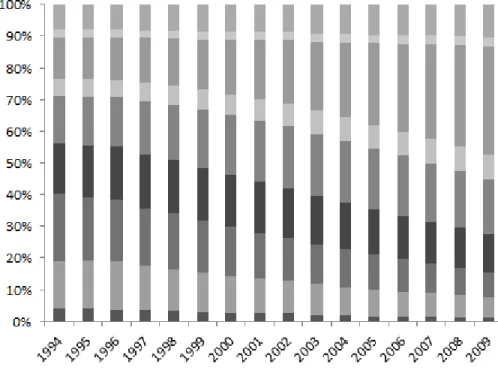
The sample’s education profile is presented in Figure 3 and shows the
per-centage of individuals by their levels of schooling. The perper-centage of individuals
with at most elementary education decreased during the period. This
reduc-tion is attributable mainly to the decline in the percentage of individuals who
had not finished the first cycle (up to 5th grade) of elementary education and
of individuals who managed to finish this cycle only. In addition, the
percent-age of individuals who had finished high school increased significantly during
the period, which is consistent with the increase in the educational level of the
workforce observed during the period.
The RAIS reports individuals’ monthly wages in December of every year in
minimum wage units for the period analyzed (1994 to 2009). Because
mini-mum wage values vary across years, workers’ wages were converted to Brazilian
currency units (Reais) using the nominal value of the minimum wage from
De-cember of the corresponding year. Real values were obtained using the Brazilian
Consumer Price Index (INPC) from the Brazilian Census Bureau (IBGE). The weekly real wage is obtained by dividing the monthly wage by contracted weekly
working hours. The weekly real wage is reported in 2009 Reais (R$). Table C.3
in Appendix C presents descriptive statistics of the log of real weekly wages
and shows that the mean of the log of the real weekly wage increased during
the period as did its minimum and its maximum values. On average, wages
increased 0.17 log−points between 1994 and 2009.
Given these wage data, it is possible to compute the covariance matrix of the
(within-group age and education level) log of real weekly wage for December of
each year. They are obtained as residuals from cross-sectional regressions of the
log of real weekly wages on the age and education indicator variables. In this case, because information on age and education is also necessary, some
obser-vations with missing age or education information were lost, leaving 1,869,446
individuals with valid information. The covariance matrix is presented in Table
C.4 in Appendix C.
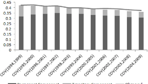
Figures 4 and 5 presents variances and selected covariances (one-, five- and
Figure 3: Descriptive Statistics: Education. Source: Elaborated by the authors. Annual Reports of Social Information (RAIS).
(Figure 5).
Figure 4: Covariances of the log of the real weekly wage. Behavior of Inequality Measured by Variance and Covariance. Source: Elaborated by the authors. Annual Reports of Social Information (RAIS).
using Brazilian National Household Surveys (PNAD/IBGE). Our goal is to ex-plain what factors led to this inequality decrease by considering the relative
importance of the permanent and transitory components associated with these
changes. The trends depicted in Figures 4 and 5 can give us some hint of
that. As time passes, the effects of transitory shocks eventually disappear. It
is plausible to consider that the larger the interval for the covariance, the more
important is the role played by the permanent component. Figures 4 and 5
illustrate the covariance for some numbers from previous periods (lags). It is
notable that covariance values remain high and relatively close to the variance
values after a number of periods, indicating that the permanent component is
Figure 5: Covariance of the residuals. Behavior of Inequality Measured by Variance and Co-variance. Source: Elaborated by the authors. Annual Reports of Social Information (RAIS).
5. Results
5.1. Wage Inequality within Age and Schooling Groups
5.1.1. Model Selection
We tested multiple specifications to estimate the covariance structure of the
log of the real weekly wage within age and schooling groups13. The estimations
were obtained using the modified weighted minimum distance method
(equa-tions 18 and 24). The different models can be compared by their chi-squared
statistics. Table 2 presents the chi-squared statistics for all tested models.
The AR (1) specification with factor loads has the lowest chi-squared
statis-tic14. For this reason, we present the results for this model. Estimation results
13
Tested specifications include the following: the canonical model, the model with factor load, the AR(1) model with factor load, and the ARMA(1,1) model with factor load.
14
Canonical Factor Loads AR(1) with Factor Loads
ARMA(1,1) with
Factor Loads
Chi-squared
statistic 751,281.51 795,808.02 221,557.38 192,498,409,553.30
Table 2: Chi-Squared Statistics of the Tested Models. Source: Elaborated by the authors. Annual Reports of Social Information (RAIS).
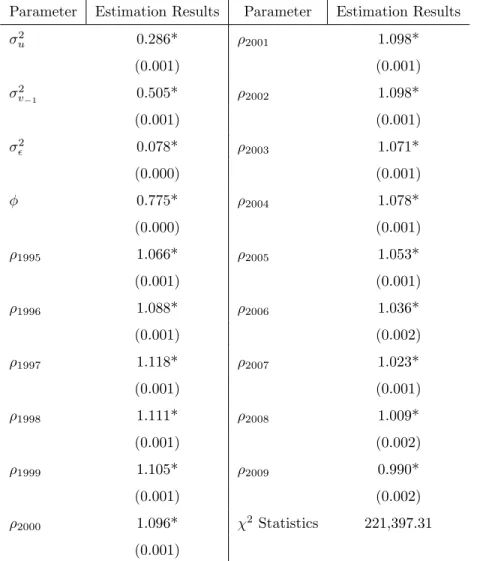
are shown in Table 3.
Note that all the included parameters are significantly different from zero at
1%. Moreover, the model is stationary. The estimated parameterφis such that
|φ|<1. Notably, the estimated returns of the permanent component (ρ) first present an upward trend until 1997 and then decrease thereafter.
5.1.2. The Decomposition of the Levels of Wage Inequality
Based on the model, we decompose the cross-sectional wage inequalities into
permanent and transitory components. The results are presented in Figure 6.
The permanent component accounts for the largest share of total cross-sectional
variance, which is 60% between 1994 and 2009, on average. The share of the
permanent component ranges from 43% in 1994 to 64% in 2002. In the final
year of the sample, this component accounted for 59.05% of the within-group wage inequality.
The overall within-group wage inequality for age and education groups
de-creases over time. The permanent component inde-creases between 1994 and 1997,
but this increase is followed by a decline in subsequent years, particularly from
2003 onwards. Changes in the permanent component are attributable to changes
in its returns. Thus, the model estimates that the return on individual
perma-nent abilities increased until 1997 and remained relatively stable until 2002,
Parameter Estimation Results Parameter Estimation Results
σ2
u 0.286* ρ2001 1.098*
(0.001) (0.001)
σ2
v−1 0.505* ρ2002 1.098*
(0.001) (0.001)
σǫ2 0.078* ρ2003 1.071*
(0.000) (0.001)
φ 0.775* ρ2004 1.078*
(0.000) (0.001)
ρ1995 1.066* ρ2005 1.053*
(0.001) (0.001)
ρ1996 1.088* ρ2006 1.036*
(0.001) (0.002)
ρ1997 1.118* ρ2007 1.023*
(0.001) (0.001)
ρ1998 1.111* ρ2008 1.009*
(0.001) (0.002)
ρ1999 1.105* ρ2009 0.990*
(0.001) (0.002)
ρ2000 1.096* χ2 Statistics 221,397.31
(0.001)
Table 3: Estimation of the AR(1) Model with Factor Load for Wage Variance within Age and Education Groups. Source: Elaborated by the authors. Annual Reports of Social Information (RAIS). Note: Standard errors in brackets. The sign * indicates significance at 1%.
where it declined steadily thereafter.
By contrast, the transitory component presents a different pattern. It
de-creases in the beginning of the analyzed period and remains stable from 2000
onwards. This pattern seems to reflect the decreasing instability and fewer
shocks in the Brazilian economy in the 1990s. Indeed, Brazil’s macro
Figure 6: Estimated Variance within Age and Schooling Groups, AR(1) with Factor Loads. Source: Elaborated by the authors. Annual Reports of Social Information (RAIS).
inflation under control, from an annual rate of 2,694% in January 1994 to 5.92%
annually in January 2001. Concurrently, a number of structural reforms were
undertaken during the same period, including privatization, economic openness,
restructuring of the financial sector, and restructuring of fiscal and monetary
policy.
Figure 7 shows the evolution of the covariances betweentand t−1 as
pre-dicted by the model. The estimated covariances decreased during the period.
The permanent component accounts for 51%, 68% and 65% of the total covari-ance in 1995, 2000 and 2009, respectively.
Figures 8 presents five-year lag period covariances. The permanent
compo-nent accounts for 80%, 85% and 85% of the total covariance in 2000, 2005 and
2009, respectively.
Finally, Figure 9 shows ten-year lag covariances.
Covariance in the 10th lag also decreased during the period from 1995
Figure 7: Estimated Covariance (Previous Period) within Age and Schooling Groups, AR (1) with Factor Loads. Source: Elaborated by the authors. Annual Reports of Social Information (RAIS).
path described for variance and covariance (previous period and 5thlag).
5.1.3. Changes in Wage Inequality
Having estimated each of the covariance components, it is now possible to
verify the extent to which each contributed to the decrease in inequality between
1994 and 2009. Table 4 contains this information.
Decrease in
Estimated Variance
Contribution
of the
Permanent
Component
Contribution
of the
Transitory
Component
Wages within Age
and Schooling Groups
28.77% 2.89% 97.11%
Figure 8: Estimated Covariance (5th Lag) within Age and Schooling Groups, AR (1) with
Factor Loads. Source: Elaborated by the authors. Annual Reports of Social Information (RAIS).
Comparing 1994 with 2009, there is a 28.77% decline in estimated total within-group variance. The change in the permanent component accounts for
2.89% of that decrease, whereas the transitory component change accounts for
97.11%. Thus, when comparing the two extreme years, the decline in wage
inequality is explained almost entirely by the decrease in transitory inequality.
Transitory inequality declined throughout the period. However, permanent
inequality presented different patterns in different periods. First, it increased
between 1994 and 1997, then became stable until 2002, and decreased thereafter.
Although the general picture seems to highlight the finding that the decrease in
wage inequality is mostly explained by the decrease in the transitory component,
the interaction between the permanent and transitory components suggests a more subtle and nuanced story. To shed light on these interactions, we further
split the overall period (1994−2009) into two sub-periods and analyze them
Figure 9: Estimated Covariance (10th
Lag) within Age and Schooling Groups, AR (1) with Factor Loads. Source: Elaborated by the authors. Annual Reports of Social Information (RAIS).
in each sub-period.
Table 5 shows the decomposition results for each period. The first
sub-period ranges from 1994 to 1997, and the second ranges from 1998 to 2009.
Although this division might seem ad hoc, we chose these sub-periods according
to the estimated trends in the permanent component. The first sub-period is
associated with an increase in the permanent component, and the second
sub-period is associated with its decrease.
Between 1994 and 1997, there is an 11.22% decrease in the estimated
vari-ance, which the transitory component fully accounted for because the permanent
component experienced an increase during the period (24.88% from its initial
value) that was more than compensated for by the decline in the transitory component (38.34% from its initial value). Table 5 illustrates this finding by
means of the negative contribution of the permanent component to the decline
Period Decline in Variance
Contribution of the
Permanent
Component
Contribution of the
Transitory
Component
1994 to 1997 11.22% -95.10% 195.10%
1998 to 2009 16.90% 74.96% 25.04%
Table 5: Decomposition of Wage Variance by Periods within Age and Schooling Groups. Source: Elaborated by the authors. Annual Reports of Social Information (RAIS).
was greater than 100%. If there were no decrease in transitory inequality, total
inequality would have increased based on the increase in permanent
inequal-ity. Alternatively, if there were no increase in permanent inequality, the total
inequality decrease would have been twice as great.
There is a different story after 1997. The (within age and education groups)
estimated variance of log-wages decreased by 16.90% between 1998 and 2009.
Our model predicts that the permanent component accounts for 74.96% of that decline and the transitory component is associated with the remaining 25.04
Notably, when the 1994−2009 period is taken as a whole, the decline in wage
inequality can almost be entirely attributed to the reduction in the transitory
component. However, when this period is split into two sub-periods, this finding
does not hold separately for each. The decrease in inequality between 1994 and
1997 results from the reduction in the transitory component alone, which seems
to be related to the decline in economic instability after implementation of the
Real Plan in Brazil. By contrast, the decrease in inequality observed in the 2000s
is mainly associated with the decrease in the permanent component through
decreases in returns on workers’ time-invariant productive characteristics over and above age and education. This finding is related to the existence of a
more stable scenario in which there is less room for reduction of the transitory
component. In conjunction with a more stable macroeconomic environment,
other forces seem to have been in place that led to the decrease in the returns
there is evidence that the decline in inequality in terms of schooling is not solely
accountable for the decrease in wage inequality resulting from the permanent
component.
6. Discussion
6.1. Mobility
The permanent component is directly associated with earnings mobility.
In-creases in this component are associated with less mobility and with a strict
labor market in which individuals seldom change positions within the wage
distribution over their lifetimes. Conversely, declines in this component are
associated with greater mobility.
We estimate that the permanent component accounts for 60% of
within-group wage inequality by age and education level, on average. This estimate
implies that individuals’ time-invariant characteristics beyond age and education largely account for their positions in the wage distribution.
The fact that the permanent component increased between 1994 and 1997
and decreased thereafter indicates that the initial position occupied by
indi-viduals in the wage distribution plays a crucial role in their potential future
positions over their lifetimes. Nonetheless, the continuous decrease in the
per-manent component throughout the 2000s suggests that long-run mobility has
increased in Brazil’s formal labor market.
6.2. The Role of Age and Education
We have documented thus far the evolution of wage inequality within age and
education groups in Brazil. A number of studies have highlighted the fact that
(unconditional) wage inequality in Latin America and, in particular, in Brazil,
is largely explained by a few observable productivity characteristics, such as
workers’ age and educational attainment and their returns (e.g., dos Reis and
distribution on the wage distribution. Specifically, we can estimate how much
of the permanent inequality is explained by observable characteristics such as
age and education.
To undertake this estimation, we perform the same permanent-transitory
decomposition for the (unconditional) log of real weekly wages using the same preferred model from the previous section15. Table 6 presents the
decomposi-tion results. The patterns are similar to those found when considering wage
inequality within age and education groups.
Period Decline in Variance
Contribution of the
Permanent
Component
Contribution of the
Transitory
Component
1994 to 2009 25.81% 29.73% 70.27%
1994 to 1997 9.70% -73.08% 173.08%
1998 to 2009 15.92% 94.99% 5.01%
Table 6: Decomposition of Wage Variance by Periods (Unconditional). Source: Elaborated by the authors. Annual Reports of Social Information (RAIS).
The unconditional log wage variance declined by almost 26% between 1994
and 2009. Among all this change, the change in the transitory component
ac-counts for 70.27% of the total change. As with the results of the log of wage
residual decomposition, the change in the transitory component entirely ac-counts for the inequality decrease in the sub-period immediately after the
econ-omy stabilized. By contrast, the change in the permanent component accounts
for 95% of the decrease in inequality in the 2000s.
Additionally, we can evaluate how much the observable characteristics of age
and education explain permanent wage inequality. LetPG be the permanent
component of the within-group wage inequality for age and education, and letP
15
be the permanent component of inequality of the unconditional log-wage. The
share of the permanent component attributed to the age and education variables
can be obtained by:
s= 1−PPG (25)
Figure 10 depicts the evolution of the share of the permanent component
attributed to age and education calculated bys.
Figure 10: Evolution of the Permanent Component Share Attributed to Age and Schooling. Source: Elaborated by the authors. Annual Reports of Social Information (RAIS).
The dispersion of the wages among age and education groups represents more than 50% of the permanent component of the log-wage variance. Notably, this
share declines sharply between 1994 and 1997 (from 59 to 53%), becomes stable
between 1998 and 2005, and increases−albeit slightly −from 2006 onward.
Although the portion of the permanent component associated with age and
education accounts for a sizable share of the permanent inequality, other
average, 46% of the permanent inequality is associated with these other factors.
Figure 11 presents the returns on permanent attributes in both situations
(unconditional wages and residual wages). The returns have similar declining
patterns throughout the period, which suggests that the returns on productive
characteristics associated with education and age as well as with other time-invariant characteristics presented the same behavior. In other words, there
appears to be a decrease in the average returns of several dimensions of human
capital (observable and non-observable) in the Brazilian formal labor market.
Figure 11: Behavior of the Returns on the Permanent Component. Source: Elaborated by the authors. Annual Reports of Social Information (RAIS).
7. Conclusion
In this study, we investigate the roles played by the permanent and
tran-sitory wage components in the evolution of wage inequality in Brazil’s formal
labor market between 1994 and 2009. Using the variance of the log of the real
weekly wage as a measure of inequality, we document that within age and
methods to assess the relative importance of permanent and transitory wage
components, we find evidence that the decrease in wage inequality stems from
the transitory component, which accounts for 97.11% of the reduction in the
variance, whereas the permanent component accounts for only 2.89% of this
decrease between 1994 and 2009. Qualitatively similar results are obtained us-ing the unconditional log of real weekly wages. Therefore, the decline in wage
inequality might be attributed to the decrease in economic instability that was
observed during the period.
Moreover, by separately assessing the evolution of inequality between 1994
and 1997 and between 1998 and 2009, we also document that the decrease in
wage inequality observed in the first sub-period results from the decrease in
the transitory component alone, a result that is likely to be associated with
the macroeconomic stability attained during this first sub-period. By contrast,
the decrease in inequality observed in the second sub-period is mainly
associ-ated with the reduction in permanent inequality. This decrease is explained by the decline in market returns on individuals’ observable and unobservable
productivity characteristics.
These findings are comparable with those of other studies on the evolution
of wage inequality in developed countries. With respect to the United States,
a number of studies document an increase in wage inequality between the late
1960s and the early 1990s. The permanent and transitory components each
account for approximately 50% of this increase in inequality. Haider (2001)
[25] investigates this period as a whole and attributes the results to skill-biased
technological changes, to the expansion of international trade, and to the effect
of education, which accounts for roughly one-third of the permanent compo-nent. Moffitt and Gottschalk (2011) [39] analyze the 1970s and 1980s and also
find that both components contributed equally to the increase in inequality. In
another study, Moffitt and Gottschalk (2012) [40] extend the study period to
2004. The authors highlight the role of the transitory component in explaining
the increase in wage inequality that was observed in the 1970s and 1980s −
per-manent component, which had a remarkable increase after the mid-1990s and
accounted for two-thirds of the increase in wage inequality that was observed
thereafter. Studies on the United Kingdom also show that both components
contributed equally to the increase in inequality between the 1970s and 1990s
(Dickens (2000) [15]). In the early 1990s, the permanent component predom-inated but later lost ground in favor of the transitory component during the
same decade (Ramos (2003) [42]). Finally, in a study of Canada for the period
between 1976 and 1992, Baker and Solon (2003) [4] also demonstrated that
both components were equally important for the increase in wage inequality.
Note that the results for Brazil during the 1994−2009 period differ from
those reported for developed countries. Although there has been an increase in
wage inequality in developed countries in recent decades, Brazil experienced a
decrease in wage inequality during the same period. Notably, the proportion of
change attributed to each component is not as well-balanced as it is in developed
countries in which each component accounts for approximately 50% of the wage variation. When explaining the decrease in formal wage inequality in Brazil, the
transitory component effect completely explains the wage inequality decrease
between 1994 and 1997 (the period immediately after the stabilization of the
economy), whereas the permanent component effect prevails in the 2000s.
Furthermore, the permanent component of the wage inequality within age
and education groups is compared with that of unconditional wage inequality
to examine the importance of the increase in schooling on inequality,. We find
that age and formal education account for approximately 54% of permanent
inequality between 1994 and 2009.
These findings contribute to the debate on the underlying causes of the de-crease in wage inequality in the Latin American region and suggest that the end
of macroeconomic instability was a relevant factor in reducing inequality. Thus,
the maintenance of macroeconomic stability in the region seems to be important
for reasons of inequality in addition to myriad other reasons. Moreover,
perma-nent changes in the labor market in the 2000s seem to have occurred over and
unobservable skills suggests that the relative demand for lower-skilled workers
increased during the period.
References
[1] Abowd, J. M. and Card, D. (1989). On the covariance structure of earnings and hours changes. Econometrica, 57(2):411–445.
[2] Azevedo, J. P., Inchauste, G., and Sanfelice, V. (2013). Decomposing the
re-cent inequality decline in latin america.World Bank Policy Research Working
Paper, (6715).
[3] Baker, M. (1997). Growth-rate heterogeneity and the covariance structure
of life-cycle earnings. Journal of Labor Economics, pages 338–375.
[4] Baker, M., Solon, G., et al. (2003). Earnings dynamics and inequality among
canadian men, 1976-1992: Evidence from longitudinal income tax records.
Journal of Labor Economics, 21(2):267–288.
[5] Barros, R. P. d., Corseuil, C., Mendon¸ca, R., and Reis, M. C. (2000).
Poverty, inequality and macroeconomic instability.
[6] Beaudry, P. and Green, D. A. (2000). Cohort patterns in canadian earnings:
assessing the role of skill premia in inequality trends. Canadian Journal of
Economics/Revue canadienne d’´economique, 33(4):907–936.
[7] Blundell, R., Graber, M., and Mogstad, M. (2014). Labor income dynamics
and the insurance from taxes, transfers, and the family. Journal of Public
Economics.
[8] Blundell, R. and Preston, I. (1998). Consumption inequality and income
uncertainty. quarterly Journal of Economics, pages 603–640.
[9] Bonhomme, S. and Robin, J.-M. (2010). Generalized non-parametric
decon-volution with an application to earnings dynamics. The Review of Economic
[10] Cappellari, L. (2000). The dynamics and inequality of Italian male
earn-ings: permanent changes or transitory fluctuations? Institute for Social and
Economic Research, University of Essex.
[11] Cardoso, E. and Urani, A. (1995). Inflation and unemployment as
deter-minants of inequality in brazil: the 1980s. InReform, Recovery, and Growth: Latin America and the Middle East, pages 151–176. University of Chicago
Press.
[12] Chamberlain, G. (1984). Panel data. Handbook of econometrics, 2:1247–
1318.
[13] Corseuil, C. H. and Foguel, M. N. (2002). Uma sugest˜ao de deflatores para
rendas obtidas a partir de algumas pesquisas domiciliares do ibge.
[14] Cysne, R. P., Maldonado, W. L., and Monteiro, P. K. (2005). Inflation
and income inequality: A shopping-time approach. Journal of Development Economics, 78(2):516–528.
[15] Dickens, R. (2000). The evolution of individual male earnings in great
britain: 1975–95. The Economic Journal, 110(460):27–49.
[16] dos Reis, J. G. A. and de Barros, R. P. (1991). Wage inequality and the
distribution of education: A study of the evolution of regional differences
in inequality in metropolitan brazil. Journal of Development Economics,
36(1):117–143.
[17] Edwards, S. (1995). Crisis and reform in latin america: From despair to
hope.
[18] Ferreira, F. H., Leite, P. G., and Wai-Poi, M. (2007). Trade liberalization,
employment flows, and wage inequality in brazil.World Bank Policy Research
Working Paper, (4108).
[19] Friedman, M. (1957). Introduction to”a theory of the consumption
func-tion”. InA theory of the consumption function, pages 1–6. Princeton
[20] Gasparini, L., Cruces, G., Tornarolli, L., and Marchionni, M. (2009). A
turning point? recent developments on inequality in latin america and the
caribbean. Technical report, CEDLAS, Universidad Nacional de La Plata.
[21] Gasparini, L., Galiani, S., Cruces, G., and Acosta, P. (2011). Educational upgrading and returns to skills in latin america: evidence from a
supply-demand framework, 1990-2010. World Bank Policy Research Working Paper,
(5921).
[22] Gonzaga, G., Menezes Filho, N., and Terra, C. (2006). Trade liberalization
and the evolution of skill earnings differentials in brazil. Journal of
Interna-tional Economics, 68(2):345–367.
[23] Gottschalk, P. and Moffitt, R. (2009). The rising instability of us earnings.
The Journal of Economic Perspectives, pages 3–24.
[24] Gottschalk, P., Moffitt, R., Katz, L. F., and Dickens, W. T. (1994). The growth of earnings instability in the us labor market. Brookings Papers on
Economic Activity, pages 217–272.
[25] Haider, S. J. (2001). Earnings instability and earnings inequality of males
in the united states: 1967–1991. Journal of Labor Economics, 19(4):799–836.
[26] Heathcote, J., Perri, F., and Violante, G. L. (2010). Unequal we stand:
An empirical analysis of economic inequality in the united states, 1967–2006.
Review of Economic Dynamics, 13(1):15–51.
[27] Heathcote, J., Storesletten, K., and Violante, G. L. (2008). The
macroeco-nomic implications of rising wage inequality in the united states. Technical report, National Bureau of Economic Research.
[28] Hryshko, D. (2012). Labor income profiles are not heterogeneous: Evidence
from income growth rates. Quantitative Economics, 3(2):177–209.
[29] Lillard, L. A. and Willis, R. J. (1978). Dynamic aspects of earning mobility.
[30] Lochner, L. and Shin, Y. (2014). Understanding earnings dynamics:
Identi-fying and estimating the changing roles of unobserved ability, permanent and
transitory shocks. Technical report, National Bureau of Economic Research.
[31] L´opez-Calva, L. F. and Lustig, N. (2010). Declining inequality in Latin America: a decade of progress? Brookings Institution Press.
[32] Lora, E. A. (2012). Structural reforms in latin america: What has been
reformed and how to measure it (updated version).
[33] Lustig, N., Lopez-Calva, L. F., and Ortiz-Juarez, E. (2013). Declining
inequality in latin america in the 2000s: the cases of argentina, brazil, and
mexico. World Development, 44:129–141.
[34] MaCurdy, T. E. (1982). The use of time series processes to model the error
structure of earnings in a longitudinal data analysis.Journal of Econometrics,
18(1):83–114.
[35] Manacorda, M., S´anchez-P´aramo, C., and Schady, N. (2010). Changes in
returns to education in latin america: The role of demand and supply of skills.
Industrial & Labor Relations Review, 63(2):307–326.
[36] McKenzie, D. and Schargrodsky, E. (2011). Buying less but shopping more:
the use of nonmarket labor during a crisis. Economia, 11(2):1–35.
[37] Meghir, C. and Pistaferri, L. (2004). Income variance dynamics and
het-erogeneity. Econometrica, 72(1):1–32.
[38] Moffitt, R. A. and Gottschalk, P. (2002). Trends in the transitory variance of earnings in the united states. The Economic Journal, 112(478):C68–C73.
[39] Moffitt, R. A. and Gottschalk, P. (2011). Trends in the covariance
struc-ture of earnings in the us: 1969–1987. The Journal of Economic Inequality,
[40] Moffitt, R. A. and Gottschalk, P. (2012). Trends in the transitory
vari-ance of male earnings: Methods and evidence. Journal of Human Resources,
47(1):204–236.
[41] Newey, W. K. (1985). Generalized method of moments specification testing.
Journal of Econometrics, 29(3):229–256.
[42] Ramos, X. (2003). The covariance structure of earnings in great britain,
1991–1999. Economica, 70(278):353–374.
[43] Rao, C. R. (1962). A note on a generalized inverse of a matrix with
applica-tions to problems in mathematical statistics. Journal of the Royal Statistical
Society. Series B (Methodological), pages 152–158.
[44] Robertson, R. (2004). Relative prices and wage inequality: evidence from
mexico. Journal of International Economics, 64(2):387–409.
[45] Robertson, R. (2007). Trade and wages: two puzzles from mexico. The World Economy, 30(9):1378–1398.
[46] Souza, A. P. (2002). Wage inequality changes in brazil: Market forces,
macroeconomic instability and labor market institutions (1981-1997).
Tech-nical report, Vanderbilt University Department of Economics.
Appendices
Appendix A
The covariance matrix of the log of wage and the covariance matrix of the elements of this matrix can be estimated following Abowd and Card (1989) [1],
except for some modifications to adjust the method to fit the unbalanced panel
case. Letyi be the deviation of the log of the real weekly wage of individuali
at t from the mean log of wages for that year. T time periods are taken into
account such that ˜yiis a 1×Tvector that contains information on the deviations
˜
yi=
yi1
yi2
.. . yiT (1)
The covariance matrix, C, is a T ×T matrix whose elements, Cjk, where
j∈[1, T] andk∈[1, T], are given by:
Cjk=
1
njk
X
i
˜
yijy˜ik (2)
where njk stands for the number of individuals who contribute to the
an-alyzed period. To define the covariance matrix of this covariance matrix, V,
define m˜ijk as the vector with the distinct elements of product ˜yijy˜ik. The
elements ofC can be estimated again by:
mjk=
1
njk
X
i
˜
mijk (3)
Finally, define ˜sijk =m˜ijk−mjk, such that the elements of the covariance
matrix of covariancejkand mn, Vjkmn wherej ∈[1, T], k∈[1, T],m∈[1, T]
andn∈[1, T], are defined by:
Vjkmn=
1
njkmn
X
i
˜
sijksimn˜ (4)
where njkmn stands for the number of individuals that contribute both to
periodjkand to periodmn. In other words,njkmnis the number of individuals
for whom there is available information on wages atj, k, mandn. Using this
approach, it is possible to calculate the observed covariance matrices, C, and
the covariance matrix of covariance,V.
Appendix B
Considering the case of the AR(1) model with factor loads, the expression
S′AS (1) where: S=
V ar(y1994)−(ρ21994σµ2+φ2σ2v−1+σ
2
ǫ)
Cov(y1994, y1995)−(ρ1994ρ1995σµ2+φ3σv2−1+φσ
2
ǫ)
Cov(y1994, y1996)−(ρ1994ρ1996σ2µ+φ4σv2−1+φ
2σ2
ǫ)
Cov(y1994, y1997)−(ρ1994ρ1997σ2µ+φ5σv2−1+φ
3σ2
ǫ)
.. .
Cov(y2008, y2009)−(ρ2008ρ2009σµ2+φ31σ2v−1+
P14
j=0φ29−2jσǫ2)
V ar(y2009)−(ρ22009σµ2+φ32σ2v−1+
P15
j=0φ2(15−j)σ2ǫ)
(2) Appendix C
Table C.1 shows an information availability matrix. The cells on the main
diagonal display the number of available observations from each year, and the
remaining cells display the number of individuals for whom there is information
for both selected years.
Tables C.2 and C.3 present descriptive statistics for the age and log of the
real weekly wages, respectively. Finally, Table C.4 shows the covariance matrix
1994 1995 1996 1997 1998 1999 2000 2001 2002 2003 2004 2005 2006 2007 2008 2009 1994 549896
1995 434616 575919
1996 403090 465020 595211
1997 381973 431062 486041 620292
1998 357522 400909 444859 504601 629965
1999 340752 380652 419726 467578 518442 642666
2000 331283 368828 404650 447352 485382 538575 675204
2001 316094 350334 383250 421639 453188 493114 550236 704528
2002 307406 340261 371254 407693 436512 471919 518669 584965 736483
2003 298561 331146 361305 395609 422804 455157 497084 547868 613805 769545
2004 292717 324911 354232 387661 413876 443869 483703 527461 580843 649825 815344
2005 285288 316533 345139 377343 402288 431217 468531 508295 555620 610584 684202 858675
2006 278210 308859 336907 368499 392347 420146 456370 493451 537076 585025 646359 723637 902808
2007 272926 302660 330288 361305 384628 411786 446932 482802 523931 567852 623734 686680 762233 957581
2008 267656 296694 323895 354362 377020 403137 437192 471669 510878 552704 605059 660229 722402 803618 1009159
2009 257376 285677 312298 341710 363832 389612 423065 455800 493637 533794 583203 634942 690248 758231 839275 1045399
Table C.1: Information Availability Matrix. Source: Elaborated by the authors. Annual Reports of Social Information (RAIS).
Year Percentage: 25 to 34 years
Percentage:
35 to 44 years
Percentage:
45 to 54 years
Percentage:
55 to 64 years Mean
Standard
Deviation
1994 0.46 0.32 0.16 0.06 37.45 9.37
1995 0.45 0.32 0.17 0.06 37.55 9.40
1996 0.45 0.32 0.17 0.06 37.63 9.45
1997 0.44 0.32 0.17 0.07 37.71 9.46
1998 0.44 0.32 0.17 0.07 37.82 9.47
1999 0.43 0.32 0.18 0.07 37.92 9.49
2000 0.43 0.32 0.18 0.07 38.01 9.51
2001 0.43 0.32 0.18 0.07 38.11 9.55
2002 0.42 0.32 0.19 0.07 38.24 9.62
2003 0.42 0.32 0.19 0.07 38.35 9.68
2004 0.42 0.32 0.19 0.08 38.41 9.74
2005 0.42 0.31 0.19 0.08 38.47 9.80
2006 0.41 0.31 0.20 0.08 38.55 9.88
2007 0.41 0.31 0.20 0.08 38.61 9.95
2008 0.41 0.30 0.20 0.09 38.71 10.02
2009 0.41 0.30 0.20 0.09 38.89 10.08
Table C.2: Descriptive Statistics: Age. Source: Elaborated by the authors. Annual Reports of Social Information (RAIS).
Year Mean Standard
Deviation Minimum Maximum
1994 3.21 1.01 0.33 9.61
1995 3.31 0.99 0.49 9.89
1996 3.33 0.98 0.55 9.77
1997 3.33 0.97 0.57 9.78
1998 3.33 0.96 0.63 9.65
1999 3.26 0.94 0.59 10.34
2000 3.27 0.93 0.65 10.18
2001 3.26 0.92 0.73 9.68
2002 3.19 0.92 0.70 9.92
2003 3.21 0.90 0.78 9.69
2004 3.22 0.90 0.80 9.71
2005 3.25 0.88 0.90 9.8
2006 3.31 0.87 1.02 9.93
2007 3.32 0.86 1.06 10.01
2008 3.35 0.86 1.08 10.25
2009 3.38 0.84 1.15 10.69
Table C.3: Descriptive Statistics: Log of the Real Weekly Wage. Source: Elaborated by the authors. Annual Reports of Social Information (RAIS).