Diogo Francisco Frederique Basílio
Licenciado em Engenharia Electrotécnica e de Computadores
Approaching the Optimal
Performance of Nonlinear OFDM
With FWA Techniques
Dissertação para obtenção do Grau de Mestre em
Engenharia Electrotécnica e de Computadores
Orientador: Prof. Doutor Rui Dinis, Professor Associado com Agregação, FCT-UNL Co-Orientador: Prof. Doutor João Francisco Martinho Lêdo Guerreiro, Professor Auxiliar na Universidade Autónoma de Lisboa
Júri:
Presidente: Prof. Doutor Luís Augusto Bica Gomes de Oliveira - FCT/UNL Arguente: Prof. Doutor Rodolfo Alexandre Duarte Oliveira - FCT/UNL Vogal: Prof. Doutor João Francisco Martinho Lêdo Guerreiro - UAL
i
Approaching the optimal performance of nonlinear OFDM using FWA techniques
Copyright © - Diogo Francisco Frederique Basílio, Faculdade de Ciências e Tecnologia, Universidade Nova de Lisboa.
A Faculdade de Ciências e Tecnologia e a Universidade Nova de Lisboa têm o direito, perpétuo e sem limites geográficos, de arquivar e publicar esta dissertação através de exemplares impressos reproduzidos em papel ou de forma digital, ou por qualquer outro meio conhecido ou que venha a ser inventado, e de a divulgar através de repositórios científicos e de admitir a sua cópia e distribuição com objetivos educacionais ou de investigação, não comerciais, desde que seja dado crédito ao autor e editor.
iii
Acknowledgements
First of all, I would like to thank Professor João Guerreiro and Professor Rui Dinis for all the help, support and readiness given for the accomplishment of this dissertation. I would also like to express my gratefulness to Faculdade de Ciências e Tecnologias da Universidade Nova de Lisboa, whose professors instructed me so well along these years. Last but not least, I’d like to thank all the people who stood by me in this journey, especially my parents.
v
Abstract
Telecommunications are part of people’s daily lives. Also, nowadays, a complete "technological illiteracy" is hard to be found in the so-called developed countries. To the point of being almost a necessity in everyday life, telecommunications must evolve to meet this need.
One of the most widely used transmission techniques in mobile communications today is Orthogonal Frequency-Division Multiplexing (OFDM). Adopted in the fourth generation of mobile communications (4G), much for its ability to deal with frequency-selective channels and good spectral efficiency, it is one of the candidate schemes to be in the fifth generation of mobile communications (5G). Despite the advantages, OFDM signals have high envelope fluctuations, making them sensitive to nonlinear effects. Several techniques were proposed to reduce these fluctuations, however they required nonlinear operations that worsened the performance of receivers. Nevertheless, it has recently been shown that the distortion effects caused by nonlinearity is no longer seen as a problem, but as information. In fact, with this discovery, it becomes possible to employ optimal receivers in order to improve the performance. Despite that, these receivers have a very high complexity and, to try to solve this problem, sub-optimal receivers have been proposed.
The sub-optimal receiver presented in this thesis is based on an optimization algorithm called Fireworks Algorithm (FWA). The thesis includes: a study of the parameters of the algorithm in order to understand its true impact on Bit Error Rate (BER) performance; a comparison of the BER for different channels: Additive White Gaussian Noise (AWGN) and Frequency-Selective; and a proposal for an FWA variant that tries to reduce the receiver’s complexity even more.
Keywords: OFDM, nonlinear effects, sub-optimal receivers, FWA, BER performance,
vii
Resumo
As telecomunicações fazem parte do quotidiano das pessoas. Nos dias de hoje, é já muito raro existir uma completa “analfabetização tecnológica” nos países ditos desenvolvidos. Chegando ao ponto de ser quase uma necessidade no dia-a-dia, as telecomunicações têm de evoluir para poderem acompanhar essa necessidade.
Uma das técnicas de transmissão mais utilizadas actualmente nas comunicações móveis é o Orthogonal Frequency-Division Multiplexing (OFDM). Adoptado na quarta geração de comunicações móveis (4G), muito pela sua capacidade de lidar com canais selectivos na frequência e boa eficiência spectral, é um dos esquemas candidatos para estar na quinta geração de comunicações móveis (5G). Apesar das vantagens, os sinais OFDM têm elevadas flutuações de envolvente, tornando-os sensíveis a efeitos de distorção não lineares. Várias técnicas foram propostas para reduzir essas flutuações, no entanto exigem operações não lineares que pioram o desempenho dos receptores. Contudo, foi recentemente demonstrado que os efeitos de distorção causados pela não linearidade deixaram de ser vistos como um problema, passando a ser tidos como informação. De facto, com esta descoberta, tornou-se possível utilizar os receptores óptimos com o objectivo de melhorar o desempenho. Todavia, este receptores apresentam uma complexidade muito elevada, sendo que para tentar resolver este problema, foram propostos os receptores sub-óptimos.
O receptor sub-óptimo apresentado nesta tese baseia-se num algoritmo de optimização chamado Fireworks Algorithm (FWA). Esta tese inclui: um estudo dos parâmetros do algoritmo de forma a entender qual o seu verdadeiro impacto no desempenho do Bit Error Ratio (BER); uma comparação desse mesmo desempenho entre dois canais diferentes: Additive White Gaussian Noise (AWGN) e Selectivo na Frequência; e uma proposta de uma variante do FWA que tenta reduzir ainda mais a complexidade no receptor.
Palavras Chave: OFDM, efeitos não lineares, receptors sub-óptimos, FWA,
ix
List of Contents
List of Acronyms ... xi
List of Symbols ... xiii
List of Tables ... xv
List of Figures ... xvii
1 Introduction ... 1
1.1Context ... 1
1.2
Objectives ... 2
2 Nonlinear OFDM ... 3
2.1OFDM fundamentals and applications ... 3
2.2
Nonlinear OFDM problems ... 7
2.3
FWA-based sub-optimal receiver ... 9
3 FWA-Based Detection for Nonlinear OFDM ... 13
3.1Explosions ... 14
3.2
Fireworks ... 16
3.2.1
B bits variation of the hard-decision sequence ... 23
3.3
Sparks ... 26
3.3.1
Maximum variation (𝜟𝑨) relative to the minimum amplitude of sparks ………..33
4 FWA’s Effects in: AWGN vs. Frequency-Selective Channels ... 39
4.1FWA’s Variant Effects ... 45
5 Conclusions ... 51
Bibliography ... 53
x
xi
List of Acronyms
ADC Analog-to-Digital Converter
AM/AM Amplitude Modulation to Amplitude Modulation
AWGN Additive White Gaussian Noise
BER Bit Error Ratio
CP Cyclic Prefix
CR Clipping Ratio
DAC Digital-to-Analog Converter
DFT Discrete Fourier Transform
DVB Digital Video Broadcasting
FDM Frequency-Division Multiplexing
FWA Fireworks Algorithm
HPA High Power Amplifier
IDFT Inverse Discrete Fourier Transform
IFFT Inverse Fast Fourier Transform
ISI Inter-symbol Interference
LTE Long Term Evolution
ML Maximum Likelihood
NL Nonlinear
OFDM Orthogonal Frequency-Division Multiplexing
P/S Parallel to Serial
PAPR Peak-to-Average Power Ratio
PTS Partial Transmit Sequence
QPSK Quadrature Phase-Shift Keying
S/P Serial to Parallel
SED Squared Euclidean Distance
SNR Signal-to-Noise Ratio
SLM Selective Mapping
xiii
List of Symbols
𝜶 Scale factor𝜟𝑨 Maximum variation relatively to 𝐴!"#
𝜟𝑷 Variation in the number of fireworks
𝜟𝑾 Maximum variation relatively to 𝑊!"#
𝓝 Normal Distribution 𝝈𝟐 Variance
𝑨 (𝒓𝒏) AM/AM conversion function
𝑨𝑴𝑰𝑵 Minimum number of sparks
B Number of bits to randomly change relatively to the hard-decision sequence 𝑫𝒌 Frequency-domain distortion terms of 𝑌!
𝒅𝒏 Nonlinear distortion terms of 𝑦! 𝑫𝑷𝟐 SED of a given firework
𝑬𝒃
𝑵𝟎 Energy per Bit to Noise Power Spectral Density Ratio
E Number of explosions
𝑬 Average number of explosions (FWA variant) 𝒇𝒔 Symbol rate
M Oversampling factor
N Number of subcarriers
𝑵𝒃𝒊𝒕 Bits transmitted per OFDM block 𝒑 𝒓 Rayleigh distribution of 𝑟!
P Number of fireworks 𝑷𝒃 Bit error probability
𝒓𝒏 Absolute value of 𝑆!
𝑺 Gaussian random variable
s Set of all transmitted sequences 𝑺𝒌 Hard-decision sequence
𝑺𝒌 Modulated subcarriers in frequency-domain
𝑺𝑴 Clipping level
𝑺𝒏 Time-domain samples of OFDM symbols
𝑻𝒔 Symbol duration time
𝒀𝒌 Frequency-domain output for the kth subcarrier
xiv
xv
List of Tables
xvii
List of Figures
FIGURE 2.1 - A.) FDM B.) OFDM; SOURCE: [16] ... 3
FIGURE 2.2 - OFDM SYMBOL WITH CYCLIC PREFIX IN TIME DOMAIN; SOURCE: [15] ... 4
FIGURE 2.3 - A.) SPECTRUM OF ORTHOGONAL SUBCARRIERS B.) TIME DOMAIN REPRESENTATION OF ORTHOGONAL SUBCARRIERS; SOURCE: [17] ... 5
FIGURE 2.4 - GENERAL OFDM SCHEME ... 6
FIGURE 2.5 - OFDM SIGNAL ENVELOPE; SOURCE: (J. GUERREIRO, PERSONAL COMMUNICATION, FEBRUARY 2, 2018) ... 7
FIGURE 2.6 - GOOD FIREWORK AND BAD FIREWORK; SOURCE: [4] ... 11
FIGURE 3.1 - SUB-OPTIMAL RECEIVER’S BER WHEN E = 1, E = 10, E = 20 AND E = 30. ... 15
FIGURE 3.2 - SUB-OPTIMAL RECEIVER’S BER WHEN E = 1, ΔP = 10, B = 1, ΔW = 1 AND ΔA = 1. ... 16
FIGURE 3.3 - SUB-OPTIMAL RECEIVER’S BER WHEN E = 1, ΔP = 50, B = 1, ΔW = 1 AND ΔA = 1. ... 17
FIGURE 3.4 - SUB-OPTIMAL RECEIVER’S BER WHEN E = 1, ΔP = 100, B = 1, ΔW = 1 AND ΔA = 1. ... 18
FIGURE 3.5 - SUB-OPTIMAL RECEIVER’S BER WHEN E = 1, ΔP = 200, B = 1, ΔW = 1 AND ΔA = 1. ... 19
FIGURE 3.6 - SUB-OPTIMAL RECEIVER’S BER WHEN E = 3, ΔP = 10, B = 1, ΔW = 1 AND ΔA = 1. ... 20
FIGURE 3.7 - SUB-OPTIMAL RECEIVER’S BER WHEN E = 5, ΔP = 100, B = 1, ΔW = 1 AND ΔA = 1. ... 21
FIGURE 3.8 - SUB-OPTIMAL RECEIVER’S BER WHEN E = 10, ΔP = 200, B = 1, ΔW = 1 AND ΔA = 1. ... 22
FIGURE 3.9 - SUB-OPTIMAL RECEIVER’S BER WHEN E = 1, ΔP = 50, B = 5, ΔW = 1 AND ΔA = 1. ... 23
FIGURE 3.10 - SUB-OPTIMAL RECEIVER’S BER WHEN E = 1, ΔP = 50, B = 20, ΔW = 1 AND ΔA = 1. ... 24
FIGURE 3.11 - SUB-OPTIMAL RECEIVER’S BER WHEN E = 10, ΔP = 50, B = 20, ΔW = 1 AND ΔA = 1. ... 25
FIGURE 3.12 - SELECTION OF INITIAL FIREWORKS, EXPLOSION AND SELECTION OF THE NEXT FIREWORKS AS THE SPARKS WITH THE LOWER SED ... 26
FIGURE 3.13 - SUB-OPTIMAL RECEIVER’S BER WHEN E = 1, ΔP = 50, B = 1, ΔW = 5 AND ΔA = 1. ... 27
FIGURE 3.14 - SUB-OPTIMAL RECEIVER’S BER WHEN E = 1, ΔP = 50, B = 1, ΔW = 10 AND ΔA = 1. ... 28
FIGURE 3.15 - SUB-OPTIMAL RECEIVER’S BER WHEN E = 1, ΔP = 50, B = 1, ΔW = 20 AND ΔA = 1. ... 29
FIGURE 3.16 - SUB-OPTIMAL RECEIVER’S BER WHEN E = 3, ΔP = 50, B = 1, ΔW = 5 AND ΔA = 1. ... 30
FIGURE 3.17 - SUB-OPTIMAL RECEIVER’S BER WHEN E = 5, ΔP = 50, B = 1, ΔW = 10 AND ΔA = 1. ... 31
FIGURE 3.18 - SUB-OPTIMAL RECEIVER’S BER WHEN E = 10, ΔP = 50, B = 1, ΔW = 20 AND ΔA = 1. ... 32
FIGURE 3.19 - SUB-OPTIMAL RECEIVER’S BER WHEN E = 1, ΔP = 50, B = 5, ΔW = 5 AND ΔA = 5. ... 34
FIGURE 3.20 - SUB-OPTIMAL RECEIVER’S BER WHEN E = 1, ΔP = 50, B = 5, ΔW = 10 AND ΔA = 5. ... 35
FIGURE 3.21 - SUB-OPTIMAL RECEIVER’S BER WHEN E = 1, ΔP = 50, B = 5, ΔW = 15 AND ΔA = 10. ... 36
FIGURE 3.22 - SUB-OPTIMAL RECEIVER’S BER WHEN E = 5, ΔP = 50, B = 5, ΔW = 5 AND ΔA = 5. ... 37
FIGURE 3.23 - SUB-OPTIMAL RECEIVER’S BER WHEN E = 10, ΔP = 50, B = 5, ΔW = 10 AND ΔA = 5. ... 38
FIGURE 4.1 - SUB-OPTIMAL RECEIVER’S BER WHEN E = 4, ΔP = 10, B = 5, ΔW = 5 AND ΔA = 5. ... 40
xviii
FIGURE 4.3 - SUB-OPTIMAL RECEIVER’S BER WHEN E = 7, ΔP= 75, B = 5, ΔW = 10 AND ΔA = 5. ... 42
FIGURE 4.4 - SUB-OPTIMAL RECEIVER’S BER WHEN E = 10, ΔP = 100, B = 5, ΔW = 15 AND ΔA = 10. ... 43
FIGURE 4.5 - SUB-OPTIMAL RECEIVER’S BER WHEN E = 20, ΔP = 100, B = 20, ΔW = 20 AND ΔA = 10. ... 44
FIGURE 4. 6 - FWA BASIC FLOWCHART WITH THE VARIANT MODIFICATIONS. ... 46
FIGURE 4. 7 - FWA WITH DYNAMIC STOPPING CRITERION: EXPLOSIONS INPUT VS. AVERAGED NUMBER OF PERFORMED EXPLOSIONS IN A OFDM TRANSMISSION. ... 48
1
1 Introduction
1.1 Context
In recent decades, we have witnessed a great evolution, and also revolution, in the wireless communications industries. The fact that these industries have grown so much in a short time is due to the ever-increasing human need to be in touch with the rest of the world, anytime, anywhere. In addition to the growth of demand for users’ mobility, this type of communications remains a challenging area due to the constant need of higher data rates and spectral efficiencies. These needs are also coupled with the desire for wireless devices with low power consumption (i.e., a long battery life) and low complexity.
In order to achieve higher data rates and spectral efficiencies, and due to their good performances over severely time-dispersive channels and low complexity receivers’ implementations, Orthogonal Frequency-Division Multiplexing (OFDM) transmission schemes emerged as one of the most popular techniques in wireless communications. However, OFDM based schemes have high envelope fluctuations, which make them very prone to nonlinear distortion effects [1], and High Peak-to-Average Power Ratio (PAPR), which leads to amplification difficulties and high-power consumption [2]. To reduce PAPR, several techniques were proposed for wireless communication systems. Some simple techniques that directly limit the peak envelope of the transmitted signal were introduced to deal with this problem. Still, the main problems of these techniques are the nonlinear distortion effects that degrade the Bit Error Ratio (BER) performance and reduce spectral efficiency. Other techniques to reduce PAPR do not introduce nonlinear problems but all of them have high computational complexities and very complex receivers, which is undesirable [3].
So, the best choice is to deal with nonlinear problems instead of complexity problems. In order to accomplish that, optimal receivers, like the maximum likelihood (ML) receiver, were designed and, in fact, they outperformed the conventional receivers used in linear conditions. The reason for this is related to the fact that the noise created by nonlinear distortion effects has some information on the transmitted signals, which can help to improve the performance [2]. However, the computational complexity of this type of receivers is still very high even considering a low number of subcarriers. To deal with the complexity and the lack of optimization of the optimal receivers, a sub-optimal receiver based on the Fireworks Algorithm (FWA) [2] [4] was proposed. It was shown that this FWA-based
2
technique allows excellent results in both performance and low-complexity, considering OFDM schemes with strong nonlinear distortion effects. This technique proved that the BER performance is even better when comparing to conventional receivers. [2]
1.2 Objectives
It was already shown that the use of FWA in nonlinear OFDM receivers leads to an improvement both in the BER performance and spectral efficiency [2]. So, the main objective of this thesis is to approach the optimal performance of nonlinear OFDM systems by understanding how each parameter influences the BER. Another objective is to compare the proposed sub-optimal receiver in two different channels: Additive White Gaussian Noise (AWGN) Vs. Frequency-selective. Finally, an FWA variant is proposed to try to reduce the complexity of the algorithm. For these purposes, all the practical aspects of this thesis will be simulated in the Matlab software.
3
2 Nonlinear OFDM
This chapter begins by describing the fundamentals of the OFDM transmission technique and its several applications in today’s world. Section 2.2 discusses the PAPR problems of OFDM transmission and some techniques that help solve these problems. Yet, these techniques create another problem: Strong nonlinear distortion effects. Section 2.3 concludes this chapter by presenting a sub-optimal receiver that can deal with OFDM signals with strong nonlinear distortion effects.
2.1 OFDM fundamentals and applications
OFDM is a multicarrier transmission technique that divides a high data rate stream, placing them onto many low rate parallel subcarriers orthogonal to each other. Thus, each subcarrier occupies less bandwidth. Since 𝑇!= !
!!, the symbol duration increases, which makes OFDM schemes less
sensitive to multipath delay spread [6] [15]. In Figure 2.1, it is possible to see the difference in spectral efficiency between OFDM and Frequency Division-Multiplexing (FDM).
4
An OFDM signal also offers robustness against selective fading, because, in the presence of interference in certain frequencies, the multicarrier system ensures that only a few subcarriers will be affected. Another advantage of OFDM is its resilience against Inter-symbol Interference (ISI). When the data is being transmitted at high rate, the bandwidth of the signal may exceed the coherence bandwidth of the channel, being the bandwidth over which the channel transfer function remains flat, causing distortion in the signal and, consequently, ISI. To deal with this problem, a guard band is added to all OFDM symbols. This guard band, called cyclic prefix (CP), consists in a part of the end of the OFDM symbol that is copied and inserted at the beginning of the next OFDM symbol in time domain. Figure 2.2 shows the OFDM symbol with CP.
Figure 2.2 - OFDM symbol with cyclic prefix in time domain; source: [15].
The main concept in OFDM is the orthogonality of the subcarriers. The orthogonality between the subcarriers allows them to be partially overlapped to each other without interference. This is, for sure, one of the best advantages that OFDM can offer: spectral efficiency. By only using an Inverse Fast Fourier Transform (IFFT) for modulation, the spacing between the subcarriers is implicitly chosen in such a way that the frequency the received signal is being evaluated at, all the other signals are zero [7]. Figure 2.3 shows the orthogonal subcarriers in frequency and time domain.
5
Figure 2.3 - a.) Spectrum of orthogonal subcarriers; b.) Time domain representation of orthogonal subcarriers; source: [17].
In order to obtain a better understanding of the OFDM scheme structure, Figure 2.4 shows a general OFDM scheme. This scheme is composed by the transmission block and a receiver block. Both blocks have the same structure but work in reverse order.
In OFDM transmission, the data stream of input bits is converted from serial to parallel and, in the next block, each parallel subcarrier is mapped into symbols in a process called modulation. Subsequently, the inverse discrete Fourier transform (IDFT) block will convert the modulated subcarriers to time domain samples. The modulated subcarriers in frequency domain are represented by {𝑆!; 𝑘 = 0, 1, … , 𝑀𝑁 − 1} and the time domain samples of the OFDM symbols by its IDFT {𝑆!= 𝐼𝐷𝐹𝑇 𝑆!; 𝑛 = 0, 1, … , 𝑀𝑁 − 1}, where M is the oversampling factor and N the number of subcarriers. Already in the time domain, the OFDM signal is converted back to serial and, thereafter, the CP is added. The OFDM signal is converted from digital to analog through a Digital-to-Analog Converter (DAC). Finally, the OFDM signal is amplified by a High-Power Amplifier (HPA), which, in this case and for the purpose of this thesis, has a nonlinear behavior, which will be explained in detail in 2.2, and transmitted to the channel. In the receiver, as already mentioned above, the OFDM signal goes through the same process in the transmission block but in reverse.
6
Figure 2.4 - General OFDM scheme.
In the 1990’s, OFDM was exploited for wideband communications and, currently, it’s used in several systems and applications that are part of people’s daily lives, such as:
• Digital Video Broadcasting (DVB)
• Wireless Personal Area Network (WPAN) access technologies IEEE 802.15.1/2/3 • Fourth generation networks as Long-Term Evolution (LTE)
The OFDM transmission technique offers not only advantages over spectral efficiency with high-data rates, but also robustness against selective fading and multipath delay spread, which makes this multicarrier modulation a major candidate for the fifth generation of wireless systems and communications [8].
7
2.2 Nonlinear OFDM problems
Despite the advantages that OFDM can offer, there are some obstacles to using this modulation scheme. One key problem of the OFDM signals is its high envelope fluctuations in time domain, which make them very sensitive to nonlinear distortion effects (Figure 2.5).
Figure 2.5 - OFDM signal envelope; source: [19].
However, the main source of nonlinear distortions is usually created by radio frequency (RF) amplifiers that deal with these high peaks, which leads to amplifications difficulties and, most important, to high power consumption.
The most classic and widely used metric to quantify the envelope fluctuations is the PAPR [9]. The PAPR is the relation between the maximum power of a sample in a certain OFDM transmitted symbol divided by the average power of that same OFDM symbol. Large PAPR occurs when the OFDM subcarriers are in-phase with each other. So, an OFDM signal consists of independently modulated subcarriers that, when added coherently, give a large PAPR. In fact, when N subcarriers are
8
added, they produce a peak power N times the average power, which leads to a very large PAPR and, consequently, making OFDM signals very prone to nonlinear distortion effects [3].
Several solutions were proposed in order to reduce the PAPR of the OFDM signals. One of the simplest solutions to deal with this problem is the clipping and filtering technique, which basically clips the OFDM signal before amplification. It was shown [10] that the lower the clipping ratio (CR) is, the greater the reduction in PAPR becomes. However, the clipping technique is a nonlinear process that may cause in-band signal distortion, resulting in BER performance degradation, and out-of-band noise, which reduces spectral efficiency. Filtering after clipping can reduce out-of-band noise but may also cause some peak re-growth. Thus, small clipping ratios reduce the effects of PAPR but, in contrast, increase nonlinear distortion effects. Other techniques without nonlinear operations were proposed in order to reduce PAPR effects in OFDM signals, such as Selective Mapping (SLM) and Partial Transmit Sequence (PTS) [11]. There are some differences between these techniques but, in general terms, both scramble an input data block of the OFDM symbols and transmit one of them with the minimum PAPR in order to reduce the probability of high PAPR. However, the computational complexity required for these techniques is extremely high, which is, for practical reasons, undesirable. Therefore, it is preferable to deal with nonlinear distortion effects than deal with high complexities.
Let us consider a nonlinear OFDM transmission. Taking the scheme shown in Figure 2.4 into account, the real and imaginary parts of OFDM time domain samples 𝑆! can be modeled by a Gaussian random variable 𝑆 ~ 𝒩 (0, 𝜎!), whose variance is 𝜎! = 1/𝑁𝑀!. An OFDM signal has an
approximately Gaussian distribution when N is sufficiently large. Therefore, the absolute value of the random variables {𝑟!= 𝑆! ; 𝑛 = 0, 1, … , 𝑀𝑁 − 1} has Rayleigh distribution, i.e.,
𝑝 𝑟 = 𝑟
𝜎!𝑒 !!!
!!! , 𝑟 > 0 (1)
Before the signal amplification, the time domain signal is submitted to an envelope clipping, which is modeled as a band-pass memoryless nonlinearity and represented by 𝑓 𝑆! = 𝐴 (𝑟!)𝑒(! !"# !! ), where 𝐴 (𝑟!) is the amplitude modulation/amplitude modulation
(AM/AM) conversion function [2],
𝐴 𝑟! = 𝑆𝑟!, 𝑟!≤ 𝑆!
9
, where 𝑆! is the clipping level. At the clipping output, the time domain samples of the nonlinearly
distorted OFDM signal can be written as {𝑦! = 𝑓 𝑆! ; 𝑛 = 0, 1, … , 𝑀𝑁 − 1}. Due to the
Gaussian-like nature of OFDM signals, the Bussgang theorem [18] is applicable. The theorem states that the cross-correlation of a Gaussian-signal before and after it passes through a nonlinear component is proportional. Therefore, the nonlinearly distorted OFDM signal can be expressed as,
𝑦! = 𝑓 𝑆! = 𝛼𝑆!+ 𝑑! , (3)
, where {𝑑!; 𝑛 = 0, 1, … , 𝑀𝑁 − 1} are the nonlinear distortion terms and 𝛼 is the scale factor given by
𝛼 =𝔼 !!!!∗]
𝔼 |!!|!]. In the receiver, by applying a discrete Fourier Transform (DFT) to {𝑦!= 𝑓 𝑆! ; 𝑛 =
0, 1, … , 𝑀𝑁 − 1}, {𝑌!; 𝑘 = 0, 1, … , 𝑀𝑁 − 1} is obtained and, for the 𝑘!! subcarrier,
𝑌! = 𝛼𝑆!+ 𝐷! , (4)
, where {𝐷!; 𝑘 = 0, 1, … , 𝑀𝑁 − 1} are the frequency domain distortion terms. Since 𝛼 < 1, the
received frequency domain block, 𝑆!, is shrunk compared to the original signal and distorted by “additive noise” terms {𝐷!; 𝑘 = 0, 1, … , 𝑀𝑁 − 1}, which can lead to a large performance degradation.
In the following section, a sub-optimal receiver based on the FWA is presented in order to counteract the nonlinearities caused by signal clipping.
2.3 FWA-based sub-optimal receiver
As mentioned in section 1.1, it was recently shown that OFDM signals with strong nonlinear distortion effects do not necessarily degrade the BER performance, because the nonlinear component has, in fact, some information on the transmitted signals that can be used to reduce performance degradation [12]. Surprisingly, nonlinear OFDM schemes can outperform linear OFDM schemes when optimal receivers are employed, such as the ML receiver [13] [14]. However, the optimal receivers are extremely complex and require a very large computer effort. Therefore, it was necessary
10
to approach the optimal performances of nonlinear OFDM schemes without all the inherent complexities of the optimal receivers.
The optimal receivers’ goal is to find the possible transmitted sequence that minimize the squared Euclidean distance (SED) relative to the received signal. However, the main problem of the optimal receivers is the lack of optimization when searching that transmitted sequence. So, to solve this problem, an FWA-based, sub-optimal receiver for nonlinear OFDM schemes was recently proposed [2].
Basically, the FWA is an iterative algorithm that consists of two phases: 1) the selection strategy phase and 2) the explosions phase. At first, P fireworks (possible transmitted sequences) are “strategically” selected from the search space s (set of all possible transmitted sequences). After the selection of the fireworks, we have a set of explosions. In each explosion, both amplitude (number of different bits) and the number of generated sparks associated with a given firework are defined by its SED, in other words, by its fitness value.
The number of generated sparks and their amplitudes play a pivotal role in this algorithm. While in the case of the number of explosions it becomes possible to exploit the search space S more than once (depending on the number of explosions), the sparks and their amplitude can be interpreted as a quality control, indicating whether the firework has a good fitness value or not. A good firework means that the explosion occurred in a location close to the optimal location of the transmitted signal. Thus, in the presence of a good firework, the use of more sparks with small amplitudes is appropriate because the solution is nearby. A bad firework means the optimal location may be far away from the location where the explosion occurred. Contrary to a good firework, a bad firework produces less sparks and larger amplitudes [2]. Figure 2.6 shows the two types of explosions that can occur. Therefore, this algorithm has the advantage of exploring the search space and, at the same time, it discards the fireworks with worse fitness values. So, with the FWA, it is possible to reduce the computational complexities of the optimal receivers.
11
Figure 2.6 – a.) Good Firework; b.) Bad Firework; source: [4].
In a more detailed explanation of this algorithm, as it was mentioned before, the first stage of FWA is the selection of the initial fireworks. There are many ways to select the initial fireworks but, in this study, the first firework is always the hard-decision sequence 𝑆!, which is the sequence associated
with the conventional receivers. The hard decision mentioned is related to the detection at the level of each subcarrier (subcarrier to subcarrier detection). After estimating the data of all the subcarriers, we get a sequence called “hard-decision”, being one of the sequences analyzed by sub-optimal detection. The rest of the initial fireworks are composed of 𝑁!"# variations of 1-bit and Δ𝑝 random variations of
B bits of the hard sequence. Therefore, 𝑃 = 𝑁!"#+ 𝛥!+ 1. The second stage of FWA is the
explosions. For each explosion, both the number of sparks and their amplitudes (number of different bits) associated with any firework 𝑝 {𝑆!(!); 𝑘 = 0, 1, … , 𝑀𝑁 − 1} are generated according to its fitness value, which is given by its SED relative to the received signal, i.e.,
𝐷!!= |𝑌!− 𝑌!(!)|! !"!!
!!!
, (5)
where {𝑌!(!); 𝑘 = 0, 1, … , 𝑀𝑁 − 1} is the nonlinear distorted version of {𝑆!(!); 𝑘 = 0, 1, … , 𝑀𝑁 − 1}. In the same explosion and for each firework, its SED is compared to the distance of the generated sparks, saving the new firework as the spark with the lower SED. In the next explosion, the sparks and their amplitudes are generated through the same process, but the new fireworks may have smaller SED
12
compared to the old ones. The cycle continues until the round of explosions is over. After a more detailed explanation on the operation of the algorithm, there are two things that should be emphasized: 1) the more explosions occur, the more likely it is to find the best possible firework; 2) the greater the variation in the number of sparks and their amplitudes is, the greater the differentiation between a good and a bad firework may be, allowing the desired transmitted sequence more easily.
In [2] it is concluded that the FWA technique applied to OFDM signals with strong nonlinear distortion effects allows better BER performances, compared to linear OFDM schemes, as well as low complexity.
13
3 FWA-Based Detection for Nonlinear OFDM
This chapter is meant to study the impact of variation of Fireworks algorithm parameters on BER performance. In addition, the BER performance of this sub-optimal receiver will always be compared with the performance for the linear case and also for the nonlinear case but with conventional receivers. The table below presents the FWA parameters to be studied:
FWA parameter
Description of parameters
E Number of explosions.
𝜟𝑷
Variation in the number of fireworks. It is the only variable that varies in 𝑃 = 𝑁!"#+ 𝛥!+ 1,
being 𝑁!"# a fixed value.
B Number of bits of the hard-decision sequence to
be randomly changed. 𝜟𝑾
Maximum variation of the number of sparks relative to the minimum number of sparks. 𝜟𝑨
Maximum variation of the amplitude of sparks relative to the minimum amplitude of sparks.
Table 3. 1 - FWA parameters and their description.
Each time a parameter is studied, all other parameters are reduced to the minimum in order to obtain its real impact on BER performance results of this FWA-based, sub-optimal receiver. Both the following results and those of chapter 4 were obtained through Monte Carlo simulations, where both perfect channel estimation and perfect frequency and time synchronization are assumed. For each Monte Carlo slot, the bit errors for the two nonlinear cases are counted, varying !!
!! from 1 to 15,
resulting in a BER plot composed by all bit error probabilities (!!
!! functions) occurred during the
Phase-14
Shift Keying Modulation (QPSK) modulation transmitted over an AWGN channel with N = 128 useful subcarriers, oversampling factor M = 4 and a normalized clipping level 𝑆! 𝜎 = 1.0. Since this variance is not constant, normalization of the clipping level is obtained by the variance of the OFDM signal. A change, for example, in the number of subcarriers N, causes 𝜎 to vary, which, in turn, changes the power of the OFDM signal, making it imperative to have such normalization in order to have a “fair” clipping level for all the cases. The minimum number and amplitude of the sparks generated in each explosion are unitary, i.e., 𝐴!"# = 𝑊!"# = 1, and they are the only parameters that
do not change during the entire study.
3.1 Explosions
One of the most important parameters of FWA is the explosions parameter. The explosions allow to determine, through the variation of the amplitude and the number of generated sparks, if the firework associated with these variations has a good fitness value or not, according to its SED to the received signal. More important than the explosion itself is the number of the explosions. The greater the number of explosions is, the greater is the possibility that the algorithm finds the best sequence according to its fitness value, having the capacity to deeply explore the search space and, at the same time, to prevent the sub-optimal receiver from an early convergence. However, the increase in the number of explosions also entails an increase in the complexity and duration of the algorithm. That being so, it is necessary to study what the best trade-off between performance and complexity will be.
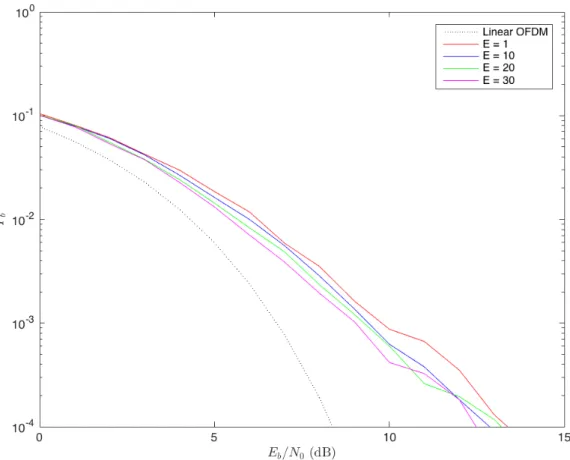
Considering the importance of this parameter in the fireworks algorithm, it was necessary to verify how the BER performance varies according to the number of explosions applied. Therefore, Figure 3.1 shows the BER performance results of the FWA-based, sub-optimal receiver when different numbers of explosions are considered and with all other parameters reduced to the minimum, plus the BER performance of a linear OFDM receiver for comparison purposes.
15
Figure 3.1 - Sub-optimal receiver’s BER when 𝐸 = 1, E = 10, 𝐸 = 20 and E = 30.
Considering the performance results shown in the figure above are just the result of the variation in the number of explosions, it is expected not to reach the full potential of the FWA. Even so, it was possible to obtain interesting results. Looking at the three curves that represent the variation in the number of explosions, the one that stands out is the curve associated with the 30 explosions, which corresponds to the pink color. Although not the best curve for all Signal-to-Noise Ratio (SNR) values due to the minimization of the remaining parameters, it gives good results especially for high SNR values. At 𝑃! = 10!!, it can reach approximately 8.8 dB, having a performance gain of 1 dB
compared to the curve associated with 𝐸 = 1.
Even though E is probably the most important parameter of the FWA, the results shown in the previous figure prove that the “help” of the other parameters is necessary to demonstrate the real effect
16
in BER performance when a considerable increase in the number of explosions is applied to the algorithm.
3.2 Fireworks
As it was mentioned in section 2.3, 𝑃 fireworks are the possible transmitted sequences, and the initial selected fireworks considered are: the hard-decision sequence (𝑆!), 𝑁!"# variations of 1-bit of 𝑆! and 𝛥! random variations of B bits of 𝑆!. In the following figures, BER performance results of
the impact of FWA receivers considering different values of 𝛥! are shown and compared to the case
of a linear OFDM transmission and a nonlinear OFDM transmission with conventional receiver.
17
Figure 3.2 shows the performance of the FWA-based, sub-optimal receiver when 𝐸 = 1, 𝛥!= 10, 𝐵 = 1, 𝛥! = 1 and 𝛥! = 1. The first value for Δ𝑝 is relatively small but it still allows some
variety to the initial fireworks. Even with all other parameters reduced to 1, with special emphasis on the explosions parameter, the performance relative to the sub-optimal receiver with FWA is better than the performance associated with the conventional receivers. At 𝑃! = 10!!, the SNR is 10.2 dB,
whereas the performance gain in relation to those conventional receivers is approximately 2.4 dB.
Figure 3.3 - Sub-optimal receiver’s BER when 𝐸 = 1, 𝛥!= 50, 𝐵 = 1, 𝛥! = 1 and 𝛥𝐴= 1.
When the 𝛥! parameter is increased to 50, there is no improvement in the performance gain over conventional receivers, as shown in Figure 3.3. Now with 𝛥! = 50, the performance gain reaches again 2.4 dB. However, for high SNR values, there is a slight improvement comparing to Figure 3.2.
18
Figure 3.4 - Sub-optimal receiver’s BER when 𝐸 = 1, 𝛥!= 100, 𝐵 = 1, 𝛥! = 1 and 𝛥𝐴= 1.
In the case of Figure 3.4, where Δ𝑝 has been increased 2 times (𝛥!= 100) in relation to the
value of the previous figure, it is possible to detect a considerable improvement in BER performance. When 𝛥!= 100, the sub-optimal receiver performance gain relative to the conventional receiver
curve, at 𝑃! = 10!!, reaches 3 dB, registering an increase of 0.6 dB compared to the two previous
19
Figure 3.5 - Sub-optimal receiver’s BER when 𝐸 = 1, 𝛥!= 200, 𝐵 = 1, 𝛥!= 1 and 𝛥𝐴= 1.
Comparing the BER performance results when Δ𝑝 = 100 with the results when 𝛥!= 200, the
performance gain increased at 𝑃! = 10!!, being 3.1 dB.
With the increase in the number of fireworks, the possibility of having a firework with a good fitness value grows. However, the amount of fireworks with a bad fitness value also grows, which indicates that increasing the number of fireworks without raising the rest of the parameters can be inefficient. This scenario can be interpreted as a way to find the best possible transmitted sequence amongst hundreds of sequences but in only an attempt and the maximum of two hints for trying to find the next sequence, making the analogy to the fact that the fireworks algorithm is exploding only once and generating a maximum of two sparks per firework.
The results obtained from this variation initially made to the Δ𝑝 parameter prove what was mentioned in the paragraph above. If only the number of fireworks increases and all other parameters keep to the minimum, the performance gain will barely be affected. Both increases and decreases in
20
gain registered in the last four figures are due to the fact that the algorithm is fortunate or not to find fireworks with good fitness value, taking into account that only one explosion is being carried out. Therefore, it is clear that only one explosion is not enough to deal with so many fireworks and the need to increase the number of explosions turns essential to better explore the search space S, which contains all the possible transmitted sequences. In what concerns the other parameters, they will be dealt later, remaining minimized.
In the next three figures, the 𝛥! parameter will vary again but differently: the explosions
parameter is no longer kept to a minimum and is also varied without changing the other parameters.
Figure 3.6 - Sub-optimal receiver’s BER when 𝐸 = 3, 𝛥!= 10, 𝐵 = 1, 𝛥!= 1 and 𝛥𝐴= 1.
Figure 3.6 shows the BER performance of this sub-optimal receiver when 𝛥!= 10 but with
𝐸 = 3. The distinction between BER performances of Figure 3.2 and the Figure 3.6 becomes evident. At 𝑃! = 10!!, the performance gain over conventional receivers is, approximately, 3.3 dB, which is
21
performance with the increase in the number of explosions from one to three, it is expected that a greater increase in the same parameter will benefit its performance. So, the next figure shows the performance results of varying 𝛥! from 10 to 100 and E from 3 to 5.
Figure 3.7 - Sub-optimal receiver’s BER when 𝐸 = 5, 𝛥!= 100, 𝐵 = 1, 𝛥! = 1 and 𝛥𝐴= 1.
Figure 3.7 shows the performance results of the proposed sub-optimal receiver when 𝐸 = 5, 𝛥!= 100, 𝐵 = 1, 𝛥!= 1 and 𝛥!= 1. For this simulation, it was decided to increase the
number of fireworks a bit more than the number of explosions relative to the value of those same parameters used in Figure 3.6. While 𝛥! increased 10 times, as it was made in Figure 3.4, the number
of explosions only increased from 3 to 5. Now, at 𝑃! = 10!!, the performance gain over conventional
receivers is 2.8 dB, which is 0.5 dB lower than when 𝐸 = 3 and 𝛥!= 10. Compared to Figure 3.6, the disproportionate increase previously achieved in the parameters in question minimized the effect of the small increase in the number of explosions in BER performance. So, for the next simulation, both
22
parameters will be increased to double the value they already had, more specifically 𝛥𝑝 = 200 and 𝐸 = 10.
Figure 3.8 - Sub-optimal receiver’s BER when 𝐸 = 10, 𝛥!= 200, 𝐵 = 1, 𝛥!= 1 and 𝛥𝐴= 1. The BER performance result of this sub-optimal receiver shown in Figure 3.8 improved a little compared to the one in the last figure. At 𝑃!= 10!!, the performance gain over the conventional
receiver is approximately 3 dB, only 0.2 dB above when 𝐸 = 5 and 𝛥!= 10. However, this gain does
not exceed the gain obtained in Figure 3.6. Even with ten explosions, the high number of 𝛥! prevented a large increase in gain, becoming exaggerated for the situation, not to mention the small influence of the other parameters derived from their minimization. At the end of the study of the impact of variation in the number of fireworks, and considering the benefits in increasing the number of explosions, it is possible to verify that only varying the 𝛥! parameter does not have as great relevance
as when also varying E. Nonetheless, a good conjugation in the variation of these two parameters can result in a better performance of the BER, further decreasing the value of 𝛥! and, on the contrary,
23
increasing even more the number of explosions. From now on and for the rest of the simulations in this section, except when it is purposely varied, 𝛥!= 50.
3.2.1 B bits variation of the hard-decision sequence
In this subsection, parameter B will be varied as well, in order to increase diversity in the initial fireworks, by randomly varying B bits corresponding to the hard-decision sequence. For this parameter, three simulations of this sub-optimal receiver will be performed: first one with 𝐵 = 5, second one with 𝐵 = 20 and the third one with 𝐵 = 20 and 𝐸 = 10. All parameters are minimized except 𝛥!, which will be, from now on, 𝛥!= 50.
24
By checking the result of BER performance of Figure 3.9, it is natural that the first comparison to be made is with the case of Figure 3.3, where the same values of the parameters are applied, except, of course, for parameter B. In relation to performance gains over conventional receivers, at 𝑃! = 10!!, the situation did not change very much, being at 2.5 dB. The random variation of only 5-bit
made to the hard-decision sequence, which is introduced in the selected initial fireworks, was not shown to be ideal for a greater performance gain. It should also be borne in mind that increasing the number of explosions boosts all other parameters. However, for the next figure, the impact of parameter B will continue to be tested without making any change in the number of explosions.
Figure 3.10 - Sub-optimal receiver’s BER when 𝐸 = 1, 𝛥!= 50, 𝐵 = 20, 𝛥!= 1 and 𝛥𝐴= 1.
The performance gain shown in Figure 3.10, for the same bit error probability and when 𝐵 = 20, reaches 3.1 dB, which is 0.6 dB above the SNR value for 𝐵 = 5 and 0.7 dB more than the gain registered for when 𝐵 = 1, 𝐸 = 1 and 𝛥!= 50 (Fig. 3.3). Even if the introduction of more
25
diversity, varying 20 bits instead of 5, gave rise to positive results, it is expected that the increase in the number of explosions will greatly improve BER performance, which can be visualized through Figure 3.11.
Figure 3.11 - Sub-optimal receiver’s BER when 𝐸 = 10, 𝛥!= 50, 𝐵 = 20, 𝛥! = 1 and 𝛥𝐴= 1. Figure 3.11 shows the sub-optimal BER when 𝐵 = 20 and 𝐸 = 10. From the figure a performance gain of 4.3 dB over conventional receivers can be observed, which is the highest gain so far. The combination between a high number of explosions and a low number of 𝛥! with a high
number of bits to be randomly changed relative to the hard-decision sequence becomes a good solution to obtain great performance gains. However, in order to release the full potential of the FWA, it is necessary to vary the number of sparks as well, hoping that a greater differentiation between what is a good or a bad firework, caused by that same variation, will benefit the performance of BER.
26
3.3 Sparks
The next parameter to be studied is the sparks one, more precisely their variation (𝛥!) relative
to the minimum number of sparks associated with each explosion, which, for this thesis, is always 𝑊 = 1. The sparks are probably the second most important parameter besides explosions. As it was mentioned before, the number of sparks generated by each explosion is given by the minimum SED of the previous fireworks. Figure 3.12 shows a more intuitive way of perceiving the purpose and importance of sparks in the system.
Figure 3.12 - Selection of initial fireworks, explosion and selection of the next fireworks made out of the sparks with the lower SED
From Figure 3.12, it is possible to verify the importance of the number of sparks in the algorithm. If the maximum variation of the number of sparks (𝛥!) in relation to their minimum value
27
sparks generated in each explosion and for each firework will only be two. Therefore, with a maximum of two sparks generated for each firework, in each explosion, the difference between a good and a bad firework will not be enlightening, which means that the algorithm does not select the following firework with the highest accuracy. For example, if the algorithm manages to find a firework with an excellent fitness value but only two sparks are generated, the difference from this firework and the fireworks with only a good fitness value will be very little. So, the trend will always be to have a considerable 𝛥! value that does not limit the differentiation between a good and a bad
firework.
As it happened in the study of the impact of the variation in the number of fireworks, a variation of the 𝛥! will be firstly chosen with all other parameters equal to one, except the 𝛥! that
will always be 50 until the end of this chapter. Then, the same variation of the 𝛥! will be repeated but
with the number of explosions varying at the same time.
Therefore, the next three figures will show the BER performance results when 𝛥! is 5, 10 and 20, respectively.
28
Figure 3.13 shows the BER performance results of the proposed FWA-based, sub-optimal receiver when 𝐸 = 1, 𝛥!= 50, 𝐵 = 1, Δ𝑊 = 5 and 𝛥! = 1. At 𝑃! = 10!!, the performance gain over
the conventional receivers is, approximately, 2.1 dB.
Figure 3.14 - Sub-optimal receiver’s BER when 𝐸 = 1, 𝛥!= 50, 𝐵 = 1, 𝛥!= 10 and 𝛥𝐴= 1. In Figure 3.14, when 𝛥!= 10, it is possible to analyse an evolution in BER performance compared to the results obtained in the previous figure. Now, when 𝑃! = 10!!, the performance gain
reaches 2.4 dB, which is 0.3 dB above the performance results when 𝛥!= 5. The following figure
29
Figure 3.15 - Sub-optimal receiver’s BER when 𝐸 = 1, 𝛥!= 50, 𝐵 = 1, 𝛥!= 20 and 𝛥𝐴 =
1.
Comparing these last three figures with their counterparts in the fireworks study (Figure 3.6, Figure 3.7 and Figure 3.8), it is shown that the increase of 𝛥! has the potential to greatly benefit BER
performance. However, the performance gain recorded in these first 𝛥! variations was not that great,
and, in case of Figure 3.13, it was even worse than in Figure 3.6 when 𝛥!= 50 and 𝛥!= 1. Even if
the variation of 𝛥!, in general, showed better results than the 𝛥! variation, the importance of sparks was not fully verified, because the number of sparks is not the only parameter that determines the firework quality. The amplitude of the sparks, which will be studied in the next subsection, is also an influential element in this aspect. This reason also explains the strange result of Figure 3.15 where, for the same bit error probability, there are two gains. The total discrepancy between 𝛥! and 𝛥! caused
30
instability in the algorithm, which did not know how to perfectly distinguish, at a certain point, the difference between a good and a bad firework.
Considering the results obtained so far in the study of the impact of sparks variation, it is imperative that the variation of this parameter is also accompanied by a variation in the amplitude of sparks. Nevertheless, before 𝛥! parameter is introduced, the impact of the variation in the number of
sparks will also be studied while the number of explosions is also changed, as it was done for the other parameters. Repeating the same process carried out in 3.1.2, three BER graphs will be simulated with 𝛥! = 5 and 𝐸 = 3, 𝛥! = 10 𝐸 = 5, 𝛥! = 20 and 𝐸 = 10, respectively.
Figure 3.16 - Sub-optimal receiver’s BER when 𝐸 = 3, 𝛥!= 50, 𝐵 = 1, 𝛥! = 5 and 𝛥𝐴= 1.
Comparing the results shown in Figure 3.16 with those in Figure 3.13, it is concluded that the increase in the number of explosions significantly improve BER performance, reaching an increase of
31
2.3 dB to the performance gain observed in the case of Figure 3.13, at 𝑃! = 10!!. Even knowing that
the algorithm, at this stage, does not differentiate the quality of fireworks perfectly, it is possible to conclude that by increasing the number of explosions, the variation in the number of sparks has a very great potential for improving BER performance.
As previously mentioned, the second case in this series of figures, which also combines both the variation in the number of explosions and the maximum variation in the number of sparks generated with respect to its minimum value, is when 𝛥!= 10 and 𝐸 = 5.
Figure 3.17 - Sub-optimal receiver’s BER when 𝐸 = 5, 𝛥!= 50, 𝐵 = 1, 𝛥!= 10 and 𝛥𝐴= 1.
Figure 3.17 shows a slight improvement in the overall gain, however, at 𝑃! = 10!!, the
performance gain over conventional receivers didn’t get better, quite the contrary. With the increase of the two parameters in relation to those in Figure 3.16, a lower gain was obtained, decreasing from 4.1
32
to 3.7 dB. Even so, the relevance of the number of explosions applied to the algorithm continues to leave its mark, always registering better results than when 𝐸 = 1. The last figure will demonstrate what happens when 𝛥! = 20 and 𝐸 = 10.
Figure 3.18 - Sub-optimal receiver’s BER when 𝐸 = 10, 𝛥!= 50, 𝐵 = 1, 𝛥!= 20 and 𝛥𝐴= 1.
The Figure above shows the sub-optimal receiver’s BER when 𝐸 = 10, 𝛥! = 50, 𝐵 =
1, 𝛥! = 20 and 𝛥!= 1. The performance gain achieved is huge, reaching 5 dB, which is the best so far. Yet, from 9 to 14 dB, due to the minimization of the rest of the parameters, the sub-optimal receiver clearly degrades. Comparing it with the gain of Figure 3.8, where 𝛥! = 200, E = 10 and
𝛥!= 1, it is definitively concluded that the number of sparks applied into the algorithm is much more preponderant than the variation in the number of fireworks. Even taking into account that there is still another parameter that helps to better determine the firework quality, it is concluded that it is
33
preferable to apply an intermediate 𝛥! value together with a high 𝛥! value, like Figure 3.18, than to
exaggeratedly increase 𝛥! and minimize 𝛥!, which is the situation in Figure 3.8.
3.3.1 Maximum variation (𝜟
𝑨) relative to the minimum amplitude of sparks
𝛥! parameter is one of two sparks parameters that also help the algorithm to better distinguish a good firework from a bad one. If a firework generates a lot of sparks with small amplitudes, it is considered to be a firework with good fitness value or, in other words, with a small SED relative to the received signal, as it was mentioned before. Taking the results obtained into consideration when only the number of sparks was varied, it does not make sense in this study to only vary the amplitude of the sparks. The idea, in this case, is to vary both the number of sparks and their amplitudes, in order to obtain better BER performance results. Therefore, the next three figures will show the sub-optimal receiver’s BER performance results when 𝛥!= 5 and 𝛥!= 5, 𝛥!= 10 and 𝛥! = 5, 𝛥! = 15 and 𝛥! = 10, respectively, with the number of explosions reduced to one. In addition, B will be incremented to five in order to add more diversity to the fireworks.
34
Figure 3.19 - Sub-optimal receiver’s BER when 𝐸 = 1, 𝛥!= 50, 𝐵 = 5, 𝛥! = 5 and 𝛥𝐴= 5. Comparing Figure 3.19 to Figure 3.13, when 𝛥! = 1, the performance gain over conventional receivers, at 𝑃! = 10!!, increased to 2.5 dB, which is a difference of 0.4 dB. An overall gain
improvement of 6 dB can be seen through the comparison of these two figures. Even though the performance gain didn’t increase considerably with the last variation of parameters, it was proven that the simultaneous variation between 𝛥! and 𝛥! helps the algorithm choose the next firework better.
35
Figure 3.20 - Sub-optimal receiver’s BER when 𝐸 = 1, 𝛥!= 50, 𝐵 = 5, 𝛥!= 10 and 𝛥𝐴= 5. Figure 3.20 shows that increasing the maximum number of sparks generated by each firework to its double while maintaining its maximum range variation benefits the overall performance gain. Now, at 𝑃! = 10!!, the gain over conventional receivers is 2.8 dB.
36
Figure 3.21 - Sub-optimal receiver’s BER when 𝐸 = 1, 𝛥!= 50, 𝐵 = 5, 𝛥!= 15 and
𝛥𝐴= 10.
In Figure 3.21, 𝛥! and 𝛥! were incremented to 10 and 15, respectively. It is observed that the performance gain for the same bit error probability is equal to the previous one. At this stage, the number of explosions must be increased again at the same time 𝛥! and 𝛥! are varied, in order to
37
Figure 3.22 - Sub-optimal receiver’s BER when 𝐸 = 5, 𝛥!= 50, 𝐵 = 5, 𝛥!= 5 and 𝛥𝐴= 5.
By adopting the same combination of parameters used in Figure 3.19, except for the variation in the number of explosions from 1 to 5, in Figure 3.22, it is possible to observe the important impact that this variance has on BER. At 𝑃! = 10!!, the performance gain increases by 1 dB compared to the
situation in Figure 3.19.
Previous results showed that the right combination of parameters is often more important than simply increasing them in the same proportion. Therefore, for the next figure, both the number of explosions and the maximum number of sparks generated will be increased to 10, while the maximum variation of amplitude remains the same value used in the latter case, just like the other parameters.
38
Figure 3.23 - Sub-optimal receiver’s BER when 𝐸 = 10, 𝛥!= 50, 𝐵 = 5, 𝛥!= 10 and 𝛥𝐴= 5. This sub-optimal receiver’s BER performance results shown in Figure 3.23 demonstrate that the combination of parameters chosen is much better than the previous one. Even though at 𝑃! = 10!!
the gain over conventional receivers only increased 0.5 dB from the previous figure, the overall gain was much better. It is also important to point out the small difference in relation to the linear curve, being, for the same probability of error, 1.2 dB, which is an excellent result.
At the end of the study of the impact of each parameter, there are a few things to point out: the number of explosions is, by far, the parameter that most influences BER performance. On the contrary, the number of fireworks applied to the algorithm is the least influential one. Even if an increase of diversity (B) in fireworks benefits BER, it is a parameter that depends a lot on the combination adopted for the other parameters. The second most important element of the algorithm is the sparks that, as previously mentioned, are divided into two parameters (𝛥! and Δ𝑊) that test the firework quality. A good combination of 𝛥!, 𝛥! and E generates excellent results in terms of
performance gain, both in relation to the curve for conventional nonlinear OFDM receivers and the curve corresponding to the linear OFDM receiver.
39
4 FWA’s Effects in: AWGN vs. Frequency-Selective
Channels
As mentioned in 2.1, OFDM can combat the multipath effect encountered in frequency-selective channels, which turns out to be the main reason why this transmission technique was designed and implemented. A channel is said to be frequency-selective when it exhibits constant gain and linear phase over a smaller bandwidth (coherence bandwidth) rather than the bandwidth of the signal. In other words, in frequency domain, frequency-selective channels are the ones that have a much smaller coherence bandwidth than the bandwidth of the signal. In time domain, this phenomenon is characterized by the delay spread, which is inversely proportional to the coherence bandwidth. So, the shorter the delay spread is, the larger the coherence bandwidth is.
Due to the fact that OFDM transmissions are robust against frequency-selective channels, it becomes imperative to know how the sub-optimal receiver proposed in this thesis behaves when the channel is frequency-selective. For each transmission, there will again be a comparison between the curves previously used in this thesis: linear OFDM, nonlinear OFDM with conventional receivers and nonlinear OFDM with sub-optimal receiver based on FWA, but for two types of channels: frequency-selective channels and AWGN channels. So, the idea of this section is to generate BER curves for the three cases mentioned above, comparing them both for frequency-selective channels and for AWGN channels, and also changing, in each simulation, the combination of the FWA parameters in order to obtain better performances.
40
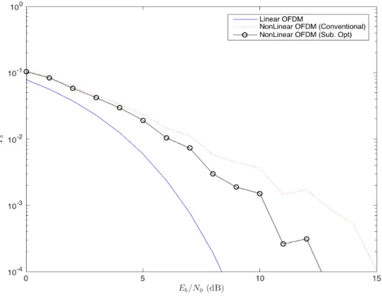
Figure 4.1 - Sub-optimal receiver’s BER when 𝐸 = 4, 𝛥!= 10, 𝐵 = 5, 𝛥!= 5 and 𝛥𝐴= 5.
Figure 4.1 shows the BER performance of the proposed sub-optimal receiver when 𝐸 = 4, 𝛥! = 10, 𝐵 = 5, 𝛥!= 5 and 𝛥!= 5. From these results it can be noted that for the case of ideal
AWGN channels, the performance gain over conventional receivers is much better, being it 2.5 dB, at 𝑃! = 10!!. For the same error probability, the gain of the linear curve over the sub-optimal receiver’s
curve is approximately 2 dB. Regarding frequency-selective channels, even with a combination of parameters with small values, the performance of this FWA-based, sub-optimal receiver can be even better than the performance of linear OFDM, particularly from 9 to 15 dB. For the next figure, the combination of parameters adopted is practically the same as the previous one, being only different in two parameters: 𝐸 = 5 and 𝛥!= 50.
41
Figure 4.2 - Sub-optimal receiver’s BER when 𝐸 = 5, 𝛥!= 50, 𝐵 = 5, 𝛥!= 5 and 𝛥𝐴= 5.
As expected, the results of the BER performance of Figure 4.2 are not so different from the results obtained in Figure 4.1. At 𝑃!= 10!!, the gain over conventional receivers increased slightly,
being approximately 3 dB, but there were no significant changes, even for frequency-selective channels. This is further evidence that a large variation in the number of fireworks only has some impact when the other parameters also accompany this variation.
42
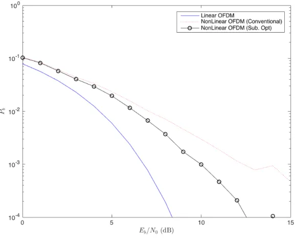
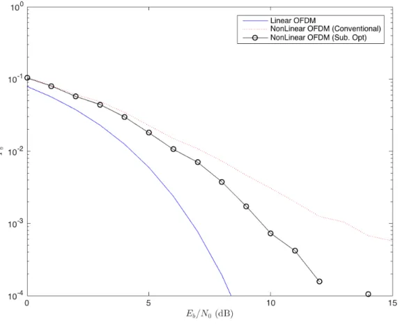
Figure 4.3 - Sub-optimal receiver’s BER when 𝐸 = 7, Δ𝑝 = 75, 𝐵 = 5, 𝛥!= 10 and 𝛥𝐴= 5. Figure 4.3 shows the sub-optimal receiver’s BER performance when 𝐸 = 7, 𝛥! = 75, 𝐵 =
5, 𝛥! = 10 and 𝛥!= 5. Note that, for this situation, both the number of explosions and 𝛥! were again
slightly increased, with the difference that, this time, the number of sparks was also increased compared to the two previous cases. Clearly, when these three parameters are varied together, the performance of this sub-optimal receiver improves considerably. In the case of AWGN channel, the performance gain over a conventional receiver increased to 4.2 dB, while the linear OFDM gain over this optimal receiver decreased to 1.2 dB. In relation to frequency-selective channels, the sub-optimal receiver’s BER performance now exceeds the linear curve at 6 dB, which is a great improvement. From now on, it is expected that, with the continuous variation in the parameters, the performance of the sub-optimal receiver will be closer to the performance of linear OFDM receivers.
43
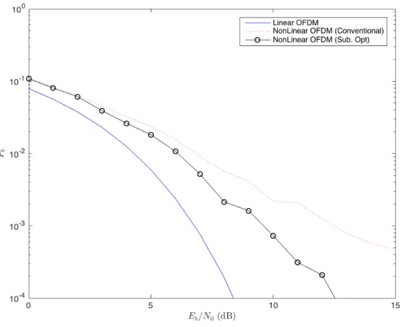
Figure 4.4 - Sub-optimal receiver’s BER when 𝐸 = 10, 𝛥!= 100, 𝐵 = 5, 𝛥!= 15 and
𝛥𝐴= 10.
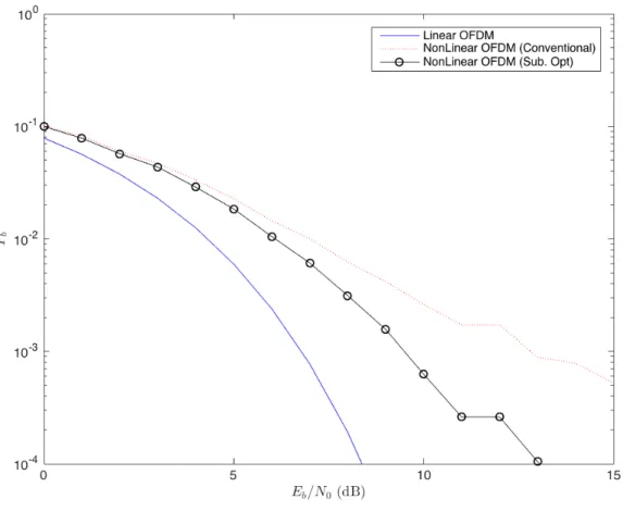
The performance results shown in Figure 4.4 were obtained by applying the following combination of parameters: 𝐸 = 10, 𝛥! = 100, 𝐵 = 5, 𝛥! = 15 and 𝛥!= 10. When 𝑃! = 10!!, the
performance gain over conventional receivers practically did not change. However, it is possible to note that the curve concerning the performance of the sub-optimal receiver in ideal AWGN channels almost reaches the linear case. For frequency-selective channels, the sub-optimal receiver’s curve surpasses the linear one at 5 dB.
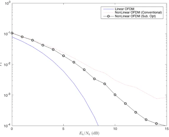
For the final figure, a more ambitious posture was adopted, increasing the parameters to the following values: 𝐸 = 20, 𝛥!= 100, 𝐵 = 20, 𝛥!= 20 and 𝛥!= 10.
44
Figure 4.5 - Sub-optimal receiver’s BER when 𝐸 = 20, 𝛥!= 100, 𝐵 = 20, 𝛥! = 20 and 𝛥𝐴= 10.
The results presented in Figure 4.5 are excellent. At AWGN channels, the performance gain of the sub-optimal receiver compared to the conventional receivers reached 6.3 dB, while between 4 and 6 dB, the sub-optimal receiver’s performance surpassed the BER performance of linear OFDM receivers. Regarding frequency-selective channels, the sub-optimal performance result achieves very large performance gain over linear OFDM, even attaining a considerable gain in relation to the conventional receivers in AWGN channels.
In the end, it is concluded that the fireworks algorithm offers excellent trade-offs between performance and complexity, especially for frequency-selective channels. A more accurate combination of the FWA parameters allows excellent BER performances. However, an exaggerated increase in all parameters, but especially more in explosions, will make the complexity much higher, which is to be avoided.
![Figure 2.3 - a.) Spectrum of orthogonal subcarriers; b.) Time domain representation of orthogonal subcarriers; source: [17]](https://thumb-eu.123doks.com/thumbv2/123dok_br/19170861.941131/25.892.124.759.139.350/figure-spectrum-orthogonal-subcarriers-domain-representation-orthogonal-subcarriers.webp)
![Figure 2.5 - OFDM signal envelope; source: [19].](https://thumb-eu.123doks.com/thumbv2/123dok_br/19170861.941131/27.892.191.662.296.697/figure-ofdm-signal-envelope-source.webp)
![Figure 2.6 – a.) Good Firework; b.) Bad Firework; source: [4].](https://thumb-eu.123doks.com/thumbv2/123dok_br/19170861.941131/31.892.185.683.125.372/figure-a-good-firework-b-bad-firework-source.webp)