Analysis of a reconfigurable UWB log-periodic antenna using the Method of Moments

Abstract— In this article we discuss in detail the numerical

implementation and computer simulations based on the Method of Moments (MoM) of the reconfigurable, ultra wideband (UWB) log-periodic antenna. The manufacturing and testing procedures are also addressed. The antenna was built utilizing low cost and/or recyclable materials and covers frequencies from 74 MHz to 2 GHz, through the discrete adjustment of its elements. The gain in a given frequency band of operation can also be changed by the reconfiguration of its elements. This antenna can be widely used in developing countries where scarce resources limit both the use of antennas in educational laboratory experiments and their use in industrial applications.

Index Terms— Wire antennas, Ultra wideband, Antenna testing and manufacturing, Method of moments.

I. INTRODUCTION

Log-Periodic Dipole Array (LPDA) antennas are the most well known log-periodic antennas [1]-[2], being used in a wide range of applications due to its broadband and narrow-beam characteristics [3]. Unfortunately, the design and construction of a LPDA antenna for ultra-wide band applications is extremely difficult. For example, it is practically impossible to build a LPDA antenna that covers VHF and UHF frequencies because of the size of the antenna and the enormous amount of dipoles it would have. Besides that, the antenna would have low portability and its installation would be expensive and complicated.

A reconfigurable log-periodic antenna makes possible to operate in many distinct frequency bands, non-simultaneously, with only one antenna through the discrete adjustment of its components and the distances between them. A reconfigurable, ultra wideband (UWB) log-periodic antenna was introduced by the authors in [4] and further discussed in [5]. The method of moments and corresponding numerical implementation are herein discussed in detail and represent the main addition over [4] and [5]. The software AS2003 [6], based on the method of moments and developed at the University of Brasilia, is employed to analyze the reconfigurable, UWB LPDA antenna [4].

Nowadays almost any problem of antenna analysis can be solved with some degree of accuracy using numerical techniques. This is due to the impressive development of digital storage capability

Analysis of a Reconfigurable UWB

Log-Periodic Antenna Using the

Method of Moments

Andre Calmon, Guilherme Pacheco, Franklin Silva and Marco Terada

Antenna Group, Electrical Engineering Dept., University of Brasilia Caixa Postal 4386 Brasilia-DF 70919-970 Brazil, fcsilva@ene.unb.br.

and computer speed occurred in the past decades. The method of moments is one of these techniques and presents the following characteristics [1]:

1) It is not necessary to impose the current distributions on the antenna geometry given that they are determined by the method.

2) All the interactions between the elements are considered when analyzing antenna arrays.

3) The method allows the analysis of elaborated antenna arrays, which are normally very difficult to analyze with other methods.

II. METHOD OF MOMENTS AND NUMERICAL IMPLEMENTATION

The main goal of the method of moments is to reduce an integral equation of the form [1]

∫

I(z')K(z,z')dz'=−Ei(z) (1) to a system of linear equations

∑

= = N n m n mnI V Z 1 (2)

which can be solved by matrix inversion yielding the current distribution

[ ] [

In Zmn

] [ ]

Vm 1 −

= (3)

From the Lorentz gauge condition

Φ − = ∂ ∂ 0

ωε

j z Az (4) and z A j E ∂ Φ ∂ − − =

ωµ

0 (5)

(1) may be written for z-direction thin wires as

) ( ' ) ' , ( ) ' , ( ) ' ( 1 /2 2 / 2 2 2 0 z E dz z z z z z z I j i z L L _ =−     Ψ + ∂ Ψ ∂

∫

− β ωε (6)

with 2 2 2 ) ' ( ) ' ( ) ' (x x y y z z

R= − + − + − , being the distance between the observation point (x,y,z) and the source point (x',y',z'). The method consists in dividing the antenna in wire segments. Using the thin wire simplification, one can set the observation point at the center of the wire and the source point on its surface. In this case R may be simplified to 2 2

) '

(z z a

R= − + , where a is the wire radius.

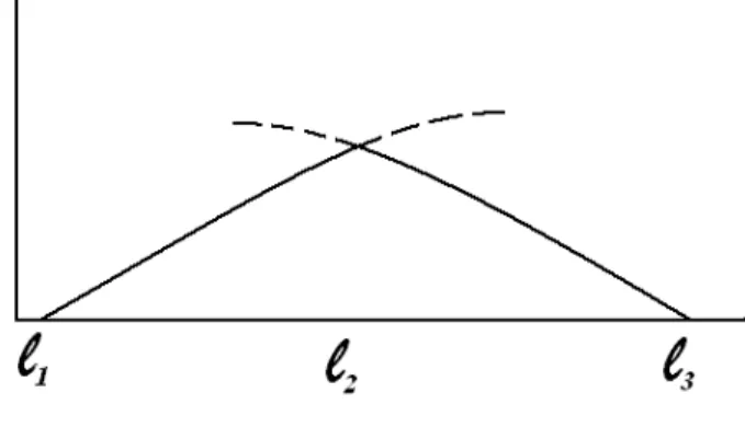
It appears impossible to solve the integral in (3), unless the I(z’) is given. However, the unknown I(z’) can be expanded as a sum of known functions, where each of the terms is multiplied by a constant. The constants become the unknowns, and the integration is numerically solved. The second member of (1) is the incident field, and it can be determinedusing known voltages in the antenna. The step of solving (1) to yield (2) may be done by using the boundary tangential conditions for the electric field along points on the wires. In this work we used the Galerkin Method [1], with the piecewise sinusoidal functions shown in Fig. 1.

Fig. 1 - Piecewise sinusoidal function

It is possible to employ others functions, such as pulses or polynomials. The preference for the piecewise sinusoidal functions stands on the fact that, in many situations, the current distribution in the log-periodic elements resembles sinusoidal functions.

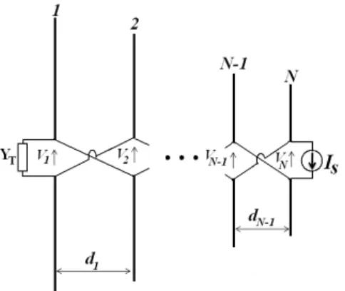
The connections between each dipole in Fig. 2 and the transmission line (antenna boon) are seen as a two port parallel connection [1,7]. Consequently, the LPDA is modeled as a parallel connection of two N-port networks, one for the dipoles and the other for the transmission line. Consequently, it is necessary to work with the admittance matrix [Ymn] instead of the impedance matrix [Zmn]. Then if the voltage matrix [VL] (L=1,2,…N) is known, the matrix [Vm] is filled and the current on the dipoles is obtained applying (3). Here, [Zmn] is computed as if the line does not exist.

Fig. 2 – Details of a log-periodic dipole antenna including the effect of reversing polarity between successive dipoles.

In order to determine [Vm] we first compute the short-circuited admittance matrix for the transmission line network, [YL] [7]:

                − + − − − + − − − − = − −1 c N1 N c 3 2 c 2 c 2 c 2 1 c 1 c 1 c 1 c T L x jY y jY 0 0 0 ... ... ... ... ... 0 ... ) x (x jY ) y jY 0 0 ... y jY ) x (x jY y jY 0 ... 0 y jY ) x jY (Y ] [Y ₍₈₎

where x_n=cot(βd_n), y_n=csc(βd_n), n=1,2,...N−1, β is the propagation constant and Yc is the characteristic admittance of the transmission line.

A new matrix [YD] is then filled with the elements of [Ymn]. For example, dividing in four segments each element of a four-element (N=4) log-periodic antenna, the [Zmn] will be a 12x12 matrix. Note that [Ymn] can be calculated inverting [Zmn], and the elements of [YD] are those that are at the feeding point of each dipole. In this case, [YD] is a 4x4 matrix. Actually, these points are the only ones where the applied voltages are not zero, since voltages are only applied at the center of each dipole. Given that the two networks are in parallel, the total current can be written as

[IS]=[[YD]+[YL]] [VL] (9) [IS] has only one element different than zero, the one which corresponds to the point where the antenna is fed; see Fig. 2. Finally, the matrix [Vm] is filled and the current distribution is obtained applying (3) as previously mentioned.

The computer code AS2003 [6] was implemented in FORTRAN with the following characteristics: 1) The numerical integration subroutines use the method of Romberg [8].

2) The inversion of the generalized impedance matrix is done by the Gauss-Jordan method [8]. 3) The adopted model for the feeding point of the log-periodic antenna is the delta-gap model

with a constant current source of unit amplitude [1].

III. COMPUTER SIMULATIONS AND EXPERIMENTAL RESULTS

The antenna has three adjustable parameters: the size of the dipoles, the distance between them and the number of elements of the antenna. This allows the antenna to be wideband and multi-band, covering practically all frequencies from 74 MHz to 2 GHz.

The dipoles were built using telescopic monopole car antennas and were soldered to hose clamps that were used to fix the monopoles to the central body, which was made of two aluminum pipes. Consequently the dipole halves could be moved along the central pipes, also made of telescopic material. Acrylic pieces fixed at the edges of the central aluminum pipes were cut permitting an adjustment in distance between the pipes. Fig. 3 shows the antenna.

Fig. 3 - Adjustable LPDA Antenna.

Table 1 lists the parameters that were obtained for the frequency band where the antenna was tested (400 to 1000 MHz). The radiation pattern in the H-plane (i.e., the plane orthogonal to the plane containing the dipoles) at a frequency of 820 MHz was simulated using the program AS2003 [6]. The computed radiation pattern of the antenna is shown in Fig. 4(a) in dB scale, whereas the measured in Fig. 4(b) in linear scale. The simulation resulted in a VSWR of approximately 2.66, a half-power angle of approximately 90 degrees and a gain of 6.29 dBi. Unfortunately, the gain of the antenna was not measured due to limitations of the available measurement equipment.

TABLEI.ANTENNAPARAMETERS(400MHZ TO1GHZ)

Element number (n) n=1 n=2 n=3 n=4 n=5 Length Ln [cm] 28.4 23.4 19.2 15.8 13.0

Spacing dn [cm] 0 8.4 6.9 5.7 4.7

Largest Elem. Radius [mm] 3.5 Central Body Length [cm] 30.0

(a) (b)

Fig. 4 - Radiation patterns (H-plane) obtained at 820 MHz: (a) computed using the method of moments code AS2003 [6] (dB scale); (b) measured (linear scale).

The antenna was fed by a coaxial cable with an impedance of 50Ω and the VSWR was measured using a slotted line connected to a transmitter with an output impedance of 50Ω. The best VSWR obtained at 820 MHz was 1.7, being better than the simulations discussed previously due to adjustments in the antenna configuration, mainly the distance between the central tubes.

IV. CONCLUSIONS

In this paper we discussed in some detail the numerical implementation and computer simulations based on the Method of Moments (MoM) of the reconfigurable, ultra wideband log-periodic antenna introduced by the authors in [4]-[5]. The manufacturing and testing procedures were also addressed. Built using low cost recycled materials, its construction details were described. Being totally reconfigurable, this antenna can cover a large range of frequencies, such as 74 MHz to 2 GHz, with different gains. Testing results were coherent with the computer simulations, validating the design.

ACKNOWLEDGMENT

This work was partially supported by CNPq (Brazilian National Research Council).

REFERENCES

[1] W. L. Stutzman and G. A. Thiele, Antenna Theory and Design, 2nd ed., New York: John Wiley, 1997.

[2] D.E. Isbell, “Log Periodic Dipole Antennas,” IRE Trans. Antennas & Propagation, Vol. AP-8, pp. 260-267, May 1960. [3] R. Carrel, “The Design of Log-Periodic Dipole Antennas,” IRE Intern. Convention Rec., Part 1, pp. 61-75, 1961. [4] A. Calmon, G. Pacheco and Marco Terada, “A Novel Reconfigurable UWB Log-Periodic Antenna”, Proceedings of the

2006 IEEE International Symposium on Antennas and Propagation, pp. 213-216, Albuquerque – NM, July 2006. [5] A. Calmon, G. Pacheco, F. Silva and Marco Terada, “A Reconfigurable UWB Log-Periodic Antenna Analyzed with the

Method of Moments", Proceedings of COMPUMAG 2007 - 16th Conference on the Computation of Electromagnetic Fields, Vol. 2, pp. 503-504, Aachen – Germany, Jun. 2007.

[6] F.C. Silva and A.J.M Soares, AS – Antenna Synthesis Code, Dept. of Electrical Engineering, University of Brasilia, 2003.

[7] R. H. Kyle, ‘Mutual coupling between log-periodic dipole antenna,” IEEE Trans. Ant. & Prop., Vol. AP-18, pp. 15-22, Jan 1970.