A numerical study on the aerodynamic performance of building cross- sections using corner modifications

A numerical study on the aerodynamic performance of building

cross-sections using corner modifications

Abstract

A numerical investigation is performed in this work in order to evaluate the aerodynamic performance of building cross-section configurations by using corner modifications. The CAARC tall building model is utilized here as ref-erence geometry, which is reshaped considering chamfered and recessed corners. The numerical scheme adopted in this work is presented and sim-ulations are carried-out to obtain the wind loads on the building structures by means of aerodynamic coefficients as well as the flow field conditions near the model’s location. The explicit two-step Taylor-Galerkin scheme is employed in the context of the finite element method, where eight-node hex-ahedral finite elements with one-point quadrature are used for spatial dis-cretization. Turbulence is described using the LES methodology, with a dy-namic sub-grid scale model. Predictions obtained here are compared with experimental and numerical investigations performed previously. Results show that the use of corner modifications can reduce significantly the aero-dynamic forces on the building structures, improve flow conditions near the building locations and increase the Strouhal number, which may have an im-portant influence on aeroelastic effects.

Keywords

Wind Engineering (WE); Computational Fluid Dynamics (CFD); Finite Ele-ment Method (FEM); Large Eddy Simulation (LES).

1 INTRODUCTION

The CAARC standard tall building model is an experimental building prototype presenting a simple hexahedral geometry with right-angle corners, which has been widely utilized to calibrate experimental methodologies in wind tunnel tests, see for instance Wardlaw & Moss (1970) and Melbourne (1980). Nevertheless, it is well known that certain geometric configurations of building corners can improve the aerodynamic performance of tall buildings by reducing the magnitude of drag and lift forces acting on the building surface. Hence, shape optimization is a major topic in building aerodynamics, where the shape of the cross-section plays an important role. In this sense, a nu-merical investigation is proposed in this work in order to evaluate the aerodynamic behavior of different cross-sections based on corner modifications applied to the CAARC geometry.

In the field of aerodynamic optimization of buildings, one can observe that significant improvements can be obtained by simply modifying the cross-section configuration slightly. In this sense, it is well known that the shape of the building corners has noticeable influence on the magnitude of aerodynamic forces acting on the building surface. Davenport (1971) is one of the first authors to investigate aspects of aerodynamic optimization applied to buildings, where different geometric configurations were analyzed. He concluded that buildings with circular cross-section behave better in terms of aerodynamic efficiency, followed by buildings with rectangular shape with modi-fied corners. Effects of the corner shape over the flow field around building models were also studied by Statho-poulos (1985) and Kwok et al. (1988) evaluated the aerodynamic performance of the CAARC tall building model by using cross-section configurations with right-angle and chamfered corners. Later, Jamieson et al. (1992) deter-mined the pressure distribution over building facades experimentally considering rectangular models and modified corners. One can see that models with rounded corners obtained the larger values in terms of maximum pressure suction in the last third of the building height. On the other hand, models with chamfered corners led to smaller pressure suction coefficients.

Tamura and Miyagi (1999) utilized two and three-dimensional building models to determine drag and lift co-efficients considering laminar and turbulent flow conditions and different corner configurations. Extensive

Guilherme Wienandts Alminhanaa_*

Alexandre Luis Brauna

Acir Mércio Loredo-Souzaa

a _{Programa de Pós-Graduação em Engenharia} Ci-vil, Universidade Federal do Rio Grande do Sul - UFRGS, Porto Alegre, RS, Brasil. E-mail: gui-lherme.alminhana@ufrgs.br, alexan-dre.braun@ufrgs.br, acir@ufrgs.br.

* Corresponding author

http://dx.doi.org/10.1590/1679-78254871 Received: January 27, 2018

experimental tests were performed by Tanaka et al. (2012) to determine the aerodynamic performance of building models with several geometric configurations. Building models with triangular shape were analyzed experimen-tally by Bandi et al. (2013), where aerodynamic coefficients and the influence of the torsion angle on the aerody-namic behavior were evaluated. The influence of corner modifications on the aeroelastic behavior of tall building models was analyzed by Kawai (1998) and Zhengwei et al. (2012). Recently, Kim et al. (2015) analyzed effects of the number of cross-section sides on the structural response of building models subject to wind action, as well as the influence of torsion as function of the building height.

With the constant improvements in the computers capability of processing data, numerical procedures of Com-putational Wind Engineering (CWE) has been successfully employed to simulate the wind action on structures (see, for instance, Blocken, 2014). Hirt et al. (1978) is one of the first authors to evaluate the aerodynamic behavior of structures numerically, where bluff bodies were analyzed and predictions compared with experimental results. Later, Hanson et al. (1982) and Summers et al. (1986) presented numerical results referring to aerodynamic anal-ysis of different structures, which are relevant to the field of Wind Engineering. In the last decades, many investi-gators have adopted the Texas Tech building model to validate their numerical models (see, for instance, Selvam, 1992; Selvam, 1996; Mochida et al., 1993; He and Song, 1997; Senthooran et al., 2004). The CAARC building model was first investigated numerically by Huang et al. (2007), where aerodynamic analyses were employed considering a finite volume scheme and different turbulence models. Later, Braun and Awruch (2009) utilized a finite element model and LES (Large Eddy Simulation) to obtain aerodynamic coefficients as well as the flow field around the CAARC building model by using aerodynamic analysis. Finally, in the field of aerodynamic optimization of buildings, one can observe that only a few works are dedicated to this subject using numerical models (see Tamura et al., 1998; Elshaer et al., 2014; Elshaer et al., 2015). Therefore, the present work proposes the use of corner modifica-tions in the CAARC prototype to evaluate aerodynamic efficiency based on standard tall building model, which is determined in terms of aerodynamic coefficients and flow conditions near to the building.

The numerical model adopted in the present simulations is presented considering an explicit two-step Taylor-Galerkin scheme, see for instance Braun and Awruch (2009). Turbulence is analyzed using LES and dynamic sub-grid scale modeling. The flow field is spatially discretized employing eight-node hexahedral finite elements with one-point quadrature and hourglass control. Building models are numerically investigated employing the standard CAARC building cross-section with corner modifications in order to obtain the aerodynamic performance of differ-ent configurations evaluating results in terms of drag and lift coefficidiffer-ents, Strouhal number, pressure and velocity fields near the model location. Predictions obtained here are compared with results provided by other authors in similar investigations.

2 FUNDAMENTAL EQUATIONS & MATHEMATICAL APPROACH

The fundamental equations of fluid flows are the momentum, mass and energy balances over the spatial do-main, which can be simplified when some physical assumptions concerning the fluid/flow behavior are considered. In the field of CWE, wind flows are usually characterized with the following assumptions:

1) Natural wind streams are considered to be within the incompressible flow range; 2) Natural wind streams are considered to be within the turbulent flow range; 3) Wind is always flowing with a constant temperature (isothermal process); 4) Gravity forces are neglected in the fluid equilibrium;

5) Air is considered mechanically as a Newtonian fluid.

The fundamental equations of the fluid domain, applying the simplifications described above, are reduced to the Navier-Stokes equations and the continuity equation (see for instance White, 1991). In the case of aerodynamic simulations, a classical Eulerian kinematical description is used and numerical difficulties in the numerical calcula-tion of turbulent incompressible flows can be avoided employing LES (Smagorinsky, 1963) and the pseudo-com-pressibility approach introduced by Chorin (1967), which leads to explicit evaluation of the pressure field. Conse-quently, the system of fundamental equations may be written as follows:

f

1 j _{, (i, j, k = 1,2,3) in}

i i t i k

j ij ij

j j j j i k

v

v _v v p v v

t x x x x x x

  

 

  

    

 _  _{ }  _    _{ }  _

 _ _ 

    _{ }  _  _

(1)

2 j _{0 (j = 1,2,3) in} f j

j j

v

p _v p _c

t x  x



 _  _{  }

where vi are components of the velocity vector v referring to xi-direction of a Cartesian orthogonal coordinate system, where xj are the corresponding components of the coordinates vector, denoted by x, ij are components of the Kroenecker’s delta,



and



are the dynamic and volumetric viscosities of the fluid, t is the eddy viscosity,

p is the thermodynamic pressure,



is the fluid specific mass, c is the sound speed in the fluid field and f is the flow spatial domain, which is bounded by f.

Neumann and Dirichlet boundary conditions must be specified on f to solve the flow problem, which are given by the following expressions:

v (i 1,2,3) on i i

v v   ₍₃₎

p

on

p p 

(4) f

σ

(i,j,k 1,2,3) on Γ

j ij j

i k i

ij j i

j i k

v n

v v t

p _{n S}

x x x

                        _ _        

  ₍₅₎

where v (boundary with prescribed velocity values vi ), p (boundary with prescribed pressure values p ) and σ

Γ (boundary with traction prescribed values Si ) are complementary subsets of the total boundary Γf, such that . In Eq. (5), nj are components of the unit normal vector n at a point located on boundary Γσ. Initial conditions for the pressure and velocity fields must be also specified at t0 to start up the flow analysis.

Turbulence modeling is performed in this work employing LES with the dynamic sub-grid scale model (see Germano et al., 1991; Lilly, 1992). The components of the Reynolds sub-grid stress tensor SGS

ij

 _{(associated with} unsolved sub-grid terms) are approximated according to the Boussinesq assumption:

 

SGS

ij i j 2 t ij   v v   S

(6) where overbars represent filtered variables and commas indicate sub-grid scale variables, t is the eddy viscosity and Sij are components of the strain rate tensor, which are expressed in terms of large scale filtered variables. The eddy viscosity is obtained employing the dynamic sub-grid scale model, which is expressed by:

 

2

t ,

 C x t  S

(7) where C x t

 

, is the dynamic coefficient (with x and t indicating space and time variables, respectively), S is the filtered strain rate tensor modulus and  _{is the characteristic dimension of the grid filter, which is associated with} element volumes for FEM schemes (_{ }3_{element volume). The dynamic coefficient C x t}

 

_{, is updated over the time} integration process considering instantaneous conditions of the flow field. The solution of Eq. (7) demands two filtering processes on the flow fundamental equations: the first filtering is associated with the classical LES formulation, which is related to the grid filter  _{and the large-scale variables. The second filtering process refers} to another filter called test filter  , which must be larger than the first grid filter _{. Variables referring to the} second filtering process are computed here using the following expression:

j n

j i j 1 _i

n j j 1 i

1               





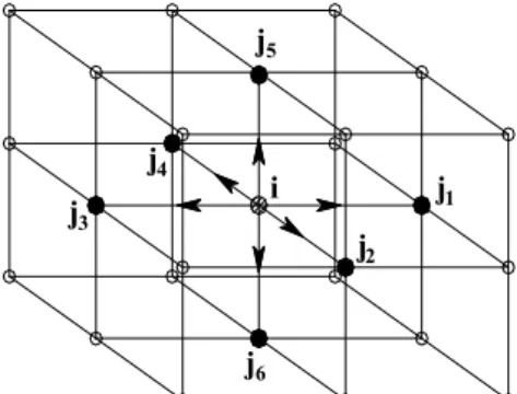
k d k d ₍₈₎

where k i is the value of a generic variable k obtained by the second filtering process at the nodal point i, which is associated with large scales defined by the first filtering process, n is the number of nodal points having direct connectivity (see Figure 1) with the nodal point i, j

i

characteristic dimension of the second filter, which is employed in the computation of the dynamic coefficient

 

,

C x t , is defined here as  = 2._.

j3 4 j j 6 j 2 i j5 j1

Figure 1: Second filter arrangement.

3 NUMERICAL MODEL

The explicit two-step Taylor-Galerkin scheme is employed in this work for time and spatial discretizations of the flow fundamental equations (see Braun and Awruch, 2009). In the present model, the Lax-Wendroff procedure is initially applied to the flow equations considering time approximations based on second-order Taylor series. In addition, a projection method proposed by Chorin (1967) is adopted, where the system of fundamental equations is resolved using a two-step fractional scheme for each time step. The numerical algorithm for the flow simulation may be summarized as follows:

(I) Solve the momentum equations to obtain a first approximation for the velocity field at the intermediate point of the time step ∆t, that is 1 2  n i v : 2

1 2 1

2 4          _{ } _  _  _  _  _ _ __  __     _{      } _ _            n j

n n i t i k i

i i j ij ij j k

j j j j i k j k

v

v v v v

t p t

v v v v v

x x x x x x x x

(9) where _t must be previously obtained from Eq. (7).

(II) Impose the boundary conditions specified by Eq. (3) and Eq. (5) on the velocity field n1 2 i v .

(III) Solve the mass conservation equation to obtain the pressure field at the intermediate point of the time step, that is _pn1 2_:

2

1 2 2

2  4

 _{ }  _  _  _       _{ } _ _{ }         n j n n

j i j

j j j i

v

t p t p

p p v c v v

x x x x

(10) (IV) Impose the boundary condition specified by Eq. (4) on the pressure field _pn1 2_.

(V) Calculate the pressure increment: 1 2 1 2

 

_pn  _pn _pn

(11) (VI) Obtain the corrected velocity field using the pressure increment calculated above, that is n1 2

i v :

2 1 2

1 2 1 2 1

8    _  _    n n n i i i t p v v x ₍₁₂₎

(VII) Impose the boundary conditions specified by Eq. (3) and Eq. (5) on the corrected velocity field n1 2 i v . (VIII) Update the velocity field using n1_ n_{ } n1 2

i i i

v v v , where:

1 2

1 2 1 _    _

                    _  _ _  _ _{ } _          n j

n i t i k

i j ij ij

j j j j i k

v

v p v v

v t r

x x x x x x

(IX) Impose the boundary conditions specified by Eq. (3) and Eq. (5) on the updated velocity field n1 i v . (X) Update the pressure field using _pn1_{ p}n_{ p}n1 2_{, where:}

1 2

1 2 _ 2

          _  _ _      n j n j j j v p

p t r c

x x

(14) (XI) Impose the boundary condition specified by Eq. (4) on the updated pressure field _pn1_.

The final arrangement of the numerical model is obtained applying the Bubnov-Galerkin’s weighted residual scheme into the FEM context on the discrete forms of the flow fundamental equations, where the weak form is considered. Eight-node hexahedral elements are adopted for spatial approximations employing one-point quadra-ture for the evaluation of element matrices. An efficient method for hourglass control is adopted according to the model proposed by Christon (1997). The system of the FEM equations in matrix notation is presented below:

 

 



n



n 1/2 n n n n

2

D

M U



_

MU

_



t

A U

_

D U F

_

(15)





n 1/2 n 1/2 n 1/2 n

i i j ij

1

4

v

v

t

a p

p







_



_





_

(16)

 



n 1/2



n 1 n * n 1/2 n 1/2 n 1/2

D

M U



_

MU

_{ }

t

_{ }

A



U



_

D U



_

F



 

₍₁₇₎

Being:

E

ij

i, j [1,8]

8

D

M









(18) i

v

U

p

 

  

 

₍₁₉₎

The vector of flow variables U is obtained using FEM approximations for velocity and pressure fields as follows:

i i i i

Φx

Φv

Φp

x

v

p







_

_

_

_

N N 1,8 N 1N 1 2N 2 3N 3

1

[ ]

1

1

1

8

Φ

 



 



 



 



 

(20)

Where Φ contains finite element interpolation functions associated with the eight-node hexahedral element. The mass matrix M is referred to as selective mass matrix, see Kawahara and Hirano (1983), which is defined as follows:



1



D

M



e

M

 

e

M

(21) Where e is the selective mass parameter, with values defined within the interval [0,1]. In this work, e is set to 0.9 for all cases analyzed.

The element matrices presented in the FEM approach used in the present work are evaluated using analytical integration, considering one-point quadrature scheme. Additional details about the FEM approach are presented in Braun e Awruch (2009).

E E V      x t c ₍₂₂₎

where xE is the characteristic dimension of element E, VE the characteristic velocity associated with element E , c is the sound speed in the physical medium and  is CFL (Courant-Friedrichs-Lewy) coefficient, which is always smaller than unity. In the present work, the time step is defined taking into account the smaller time step obtained from Eq. (22), which is related to the smaller element of the finite element mesh.

The aerodynamic coefficients are evaluated numerically considering the following expressions:

 



 











 













1 1 1 2 2 inf inf

1 _.D 1 _.D

2 2       







n _i n _i

x j j

i i

D

F t n t A

C t

V H V H

(23)

 



 











 













2 1 1 2 2 inf inf

1 _.D 1 _.D

2 2       







n _i n _i

y j j

i i

L

F t n t A

C t

V H V H

(24)

1

1 _{( )}







t

i n

D D

i

C C t

T (25)

1

1 _{( )}







nt _i

L _L

i

C C t

T _, 2

1

1







t

rms _i n L L i C C T (26)



02



inf 1 2   i i

p p p

c V (27) inf . 

t f D

S

V ₍₂₈₎

where C tD

 

and C tL

 

are the drag and lift coefficients, given as functions of time t, A is the influence area of node i,



represents the fluid density, H is the height of the model, D is a characteristic dimension of the immersed body, Vinf is the non-disturbed flow velocity and n is the number of element nodes belonging to the fluid-structure interfaceF tx

 

and F ty

 

are the resultant forces acting on node i along the X and Y directions, respectively, _{ij denotes the fluid stress tensor components, which are evaluated at the center of the element, and}

j

n are the unit normal vector components defined at node i. Time average pressure coefficient cp is defined at nodal points belonging to the fluid-structure interface, where p is the time averaged pressure at a node i of the immersed body surface and p0 is the reference pressure. The Strouhal number St is determined considering the vortex shedding frequency f , which may be obtained from power spectrum density of lift coefficient records over time. Time average values are calculated taking into account a given number of time steps nt and a given time period T.

4 NUMERICAL SIMULATION

Figure 2: Corner modifications configurations.

The computational domain adopted in numerical simulations is similar to that proposed by Braun and Awruch (2009), which is defined using the basic dimensions of the CAARC building model, that is: 180m height (H), 30m width (W) and 45m length (L). In the numerical simulation, sectional models are utilized considering the X-Y plane of the computational domain and a unit height in the z direction. In these numerical simulations, the boundary conditions imposed are: uniform flow on the inlet boundary, non-slip condition on the building surface, symmetry condition on the side boundaries and a constant gauge pressure with p = 0 on the outlet boundary.

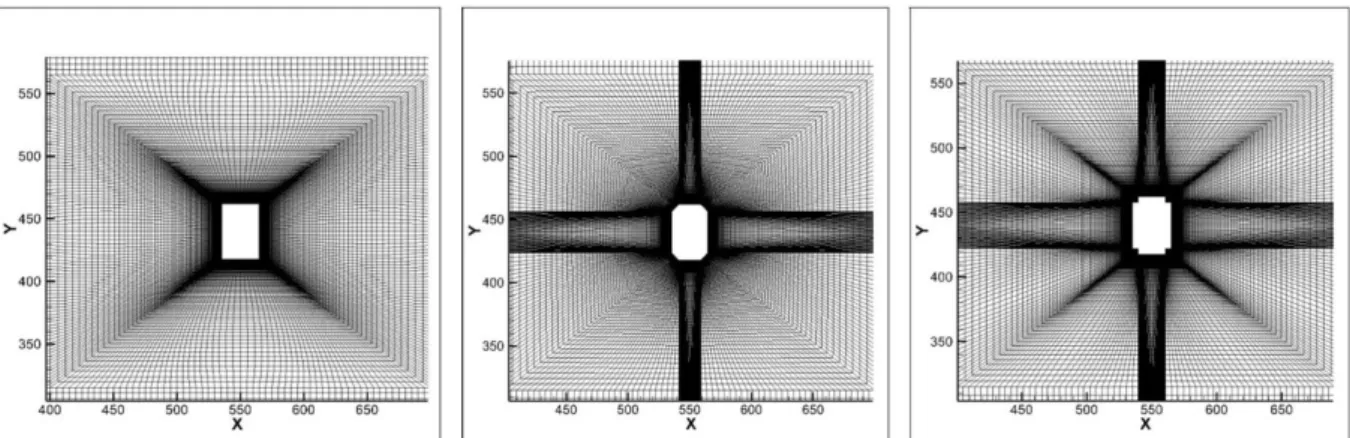
In Figure 3, details of some of the meshes used in the present investigations are shown, which correspond to the three types of corner shapes investigated here. It is important to notice that a convergence study was previously performed in order to determine the optimum mesh configuration for all the cross-section models analyzed in this work. The numerical simulations were carried out using flow parameters based on a Reynolds number of 1.2x105 and laminar inflow conditions. Mesh characteristics and flow properties utilized in the present analysis are pre-sented in Table 1 and 2, respectively. The time increment (∆t) used in simulations is defined according to the char-acteristic dimension (∆x) of the smallest element in the computational domain. In this investigation, ∆t varies from 1.5x10-3_{s to 5.0x10}-3_{s and all simulations are carried considering a period of 300s, where time averaged values are} calculated in the last 100s.

Table 1: Mesh characteristics, dimensions in cm.

Mesh characteristics

Mesh Nodes Elements Δxmín

Normal 289830 239250 7.78

Chamf. 1.5m 287160 237000 3.66

Chamf. 3.0m 287160 237000 4.22

Chamf. 4.5m 377880 312000 4.22

Chamf. 6.0m 377880 312000 5.65

Reces. 1.5m 410340 339000 2.30

Reces. 3.0m 399480 330000 3.97

Reces. 4.5m 399480 330000 5.39

Reces. 6.0m 318360 263000 5.47

Table 2: Fluid properties.

Fluid parameters General Vinf (m/s) 10.0

Mach 0.15

µ (N.s/m2_{) 3.838×10}-3 ρ (kg/m3_{) 1.0} λ (N.s/m2_{) 0.0}

D (m) 45.0

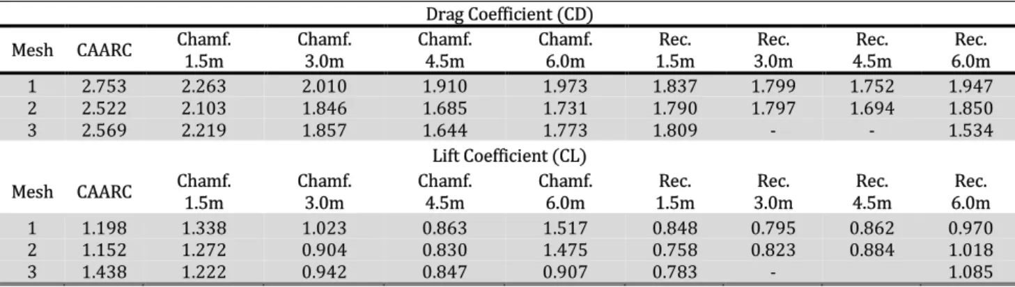
For the mesh quality study performed here, three refinement levels were adopted for all cross-section config-urations and the aerodynamic coefficients (CD and CL) were chosen as convergence parameter. The definition of the final configuration of the mesh to be used was based on the verification of which level of refinement maintained a maximum difference of about 5% in relation to the others, evaluating which level resulted in the convergence for both aerodynamic coefficients. The results of this study are presented in Table 3.

Table 3: Mesh quality study in the aerodynamic coefficients.

Drag Coefficient (CD)

Mesh CAARC Chamf. _1.5m Chamf. _3.0m Chamf. _4.5m Chamf. _{6.0m 1.5m} Rec. _3.0m Rec. _4.5m Rec. _6.0m Rec.

1 2.753 2.263 2.010 1.910 1.973 1.837 1.799 1.752 1.947

2 2.522 2.103 1.846 1.685 1.731 1.790 1.797 1.694 1.850

3 2.569 2.219 1.857 1.644 1.773 1.809 - - 1.534

Lift Coefficient (CL)

Mesh CAARC Chamf. _1.5m Chamf. _3.0m Chamf. _4.5m Chamf. _{6.0m 1.5m} Rec. _3.0m Rec. _4.5m Rec. _6.0m Rec.

1 1.198 1.338 1.023 0.863 1.517 0.848 0.795 0.862 0.970

2 1.152 1.272 0.904 0.830 1.475 0.758 0.823 0.884 1.018

3 1.438 1.222 0.942 0.847 0.907 0.783 - 1.085

Notice that the results presented above were obtained using computational grids with unitary height, where only one element is considered along Z direction of the computational domain. Taking into account the optimum meshes of the quality study, final meshes were made by discretizing the computational domain along the Z direction with five uniformly spaced elements, information about these meshes are presented in the Table 1.

5 RESULTS

5.1 Simulation results

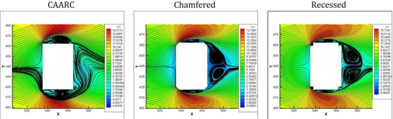
of recirculation is also identified along the back edge, indicating the presence of vortex shedding process. On the other hand, it is observed that the flow characteristics related to the chamfered configurations are noticeably influ-enced by the extension of the corner modification. For 1.5m extension, the streamlines are very similar to those obtained for the standard CAARC configuration. However, when the extension is increased, the streamlines tend to be more attached to the side edges of the body. Another noticeable remark is related to the formation of two vortices on the back edge of the chamfered models.

Figure 4: Time averaged streamlines – CAARC model and corner modification models with 1.5m, respectively.

Figure 5: Time averaged streamlines – CAARC model and corner modification models with 3.0m, respectively.

Figure 7: Time averaged streamlines – CAARC model and corner modification models with 6.0m, respectively.

One can notice that the streamlines obtained for geometric configurations related to recessed corners are dif-ferent to those associated with the standard CAARC model, even when modifications with 1.5m extension are con-sidered. By observing the flow patterns shown in the Figures 4 to 7, the geometric configurations with recessed corners generate four areas of recirculation near the corner zones. Considering the chamfered models, when the extension of corner modifications is increased the streamlines tend to attach to the lateral edges of the body as well as the two recirculation vortices along the back edge of the model tend to be larger as the extension of the corner modification is increased. However, for small extensions just one big vortex is generated.

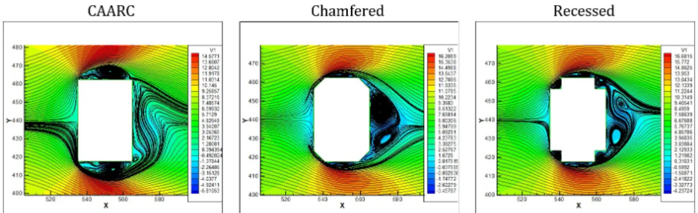
Figures 8 to 11 shows results obtained here considering the time averaged flow speed near the building con-figurations proposed in the present work. It is observed that the standard rectangular shape generates the smallest maximum flow speed, reaching the value of 14.57 m/s, while the other two shapes investigated here present values within the speed interval 15.48 - 16.68 m/s. Nevertheless, one can notice that the minimum flow speed is consid-erably influenced by corner modifications, since areas of attached flow referring to modified corners are noticeably larger than those obtained from the standard rectangular shape. Other important aspect is related to the transition observed in the flow speed. At the modified corners, transition is faster than that observed in the rectangular shape model, presenting zones that contain the smallest flow speeds.

Figure 8: Time averaged flow speed – CAARC model and corner modification models with 1.5m, respectively.

Figure 10: Time averaged flow speed – CAARC model and corner modification models with 4.5m, respectively.

Figure 11: Time averaged flow speed – CAARC model and corner modification models with 6.0m, respectively.

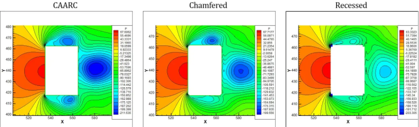
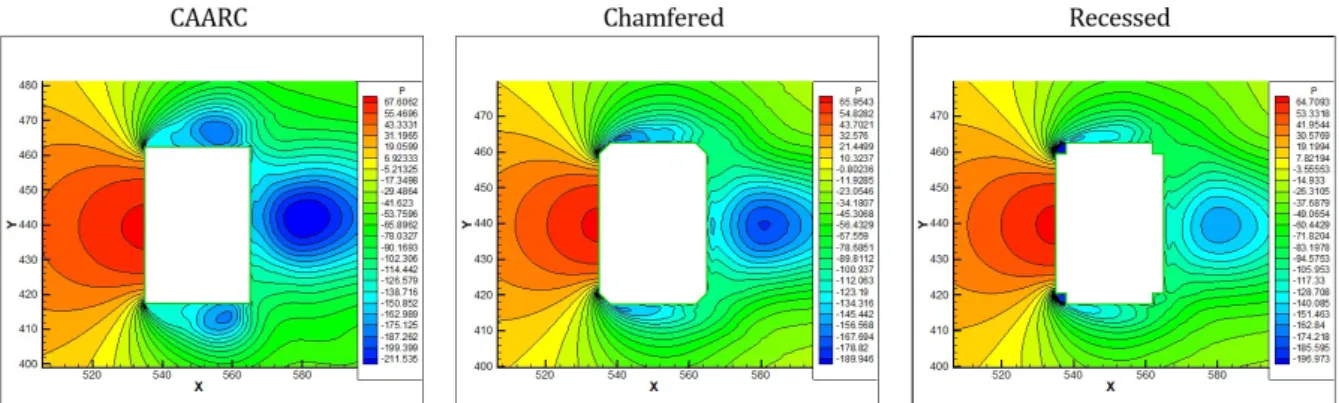
Time averaged pressure fields obtained in the present investigation are shown in Figures 12 to 15. Analyzing the flow patterns indicated by the pressure fields around the models, one can observe a similar behavior for all configurations studied here concerning the pressure distribution on the front and in the back of the models. How-ever, the major differences observed among the present results are related to the side edges of the bodies. Notice that as the extension of the corner modification is increased, zones of maximum suction begin to move upstream, which is observed for both types of modified corner configurations.

Figure 13: Time averaged pressure fields – CAARC model and corner modification models with 3.0m, respectively.

Figure 14: Time averaged pressure fields – CAARC model and corner modification models with 4.5m, respectively.

Figure 15: Time averaged pressure fields – CAARC model and corner modification models with 6.0m, respectively

In Figures 12, the cross-section configurations associated with the smallest extensions of corner modifications, the corresponding pressure fields tend to be similar to that obtained by the standard CAARC building model. At the front of the model with basic rectangular shape, the pressure field present only positive values generally, while the models with modified corners show zones with significant suction values next to the corners, which is responsible for producing a noticeable reduction in the resultant force along the flow direction.

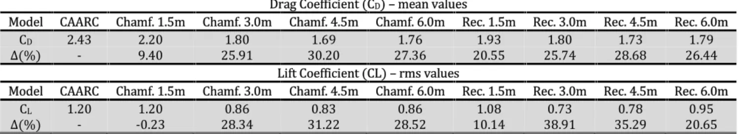
are more significant when the lift coefficient is considered, reaching values from 20.6% to 38.9% lower in the case of modifications with extension larger than 1.5m.

Table 4: Aerodynamic coefficients: mean drag value and rms lift, respectively.

Drag Coefficient (CD) – mean values

Model CAARC Chamf. 1.5m Chamf. 3.0m Chamf. 4.5m Chamf. 6.0m Rec. 1.5m Rec. 3.0m Rec. 4.5m Rec. 6.0m

CD 2.43 2.20 1.80 1.69 1.76 1.93 1.80 1.73 1.79

Δ(%) - 9.40 25.91 30.20 27.36 20.55 25.74 28.68 26.44

Lift Coefficient (CL) – rms values

Model CAARC Chamf. 1.5m Chamf. 3.0m Chamf. 4.5m Chamf. 6.0m Rec. 1.5m Rec. 3.0m Rec. 4.5m Rec. 6.0m

CL 1.20 1.20 0.86 0.83 0.86 1.08 0.73 0.78 0.95

Δ(%) - -0.23 28.34 31.22 28.52 10.14 38.91 35.29 20.65

Table 5 shows Strouhal number (St) results obtained from numerical simulations performed with the different cross-section configurations investigated. By considering the numerical predictions presented here, one can see that corner modifications lead to significant increase of vortex shedding frequency (up to 53.5%), when compared to the value obtained from the CAARC building cross-section configuration.

Table 5: Strouhal number results.

Strouhal Number (St)

CAARC Chamf. 1.5m Chamf. 3.0m Chamf. 4.5m Chamf. 6.0m Rec. 1.5m Rec. 3.0m Rec. 4.5m Rec. 6.0m

St 0.11 0.11 0.17 0.17 0.16 0.11 0.16 0.17 0.16

Δ(%) - -6.26 51.11 53.53 41.80 2.09 42.47 52.53 43.07

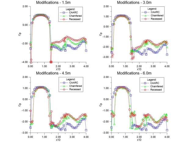
Through the pressure distributions shown in Figure 16, one can notice that pressure coefficients (cp) occur-ring along the side and back edges of the CAARC model are greater that those obtained with other corner configu-rations. The present results demonstrate that the smallest suction values referring to the standard CAARC model are found on the back edge of the model. However, suction values on the side and back edges of models with mod-ified corners are, in general, lower.

Figure 16: Pressure coefficient along model’s façades.

5.2 Results comparison

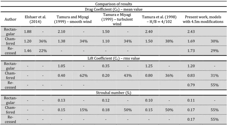
Table 6: Comparison with literature results.

Comparison of results Drag Coefficient (CD) – mean value

Author Elshaer et al. _{(2014) (1999) – smooth wind} Tamura and Miyagi (1999) – turbulent Tamura e Miyagi wind

Tamura et al. (1998)

– H/B = 4/102 with 4.5m modifications Present work, models

Rectan-gular 1.88 - 2.10 - 1.50 - 2.40 2.43

Cham-fered 1.20 36% 1.38 34% 1.10 34% 1.50 38% 1.69 30%

Re-cessed 1.46 22% - - - - 1.73 29%

Lift Coefficient (CL) – rms value

Rectan-gular - - 1.05 - 0.35 - 1.25 - 1.20 -

Cham-fered - - 0.40 62% 0.20 43% 0.80 36% 0.83 31%

Re-cessed - - - - 0.79 55%

Strouhal number (St)

Rectan-gular - - 0.13 - 0.12 - 0.10 - 0.11 -

Cham-fered - - 0.15 15% 0.18 50% 0.15 50% 0.17 55%

Re-cessed - - - 0.17 55%

The present results indicate reduction in the drag coefficient when cross-sections with corner modifications are considered, which agrees with the results obtained by other authors. In the lifting force, results obtained by the reference authors show a disagreement among them and with those obtained by the present work. Predictions reported in the literature with respect to lifting force indicate an interval of 36% to 62% reduction, while results obtained in the present work show a maximum of 31% reduction. Nevertheless, Strouhal numbers obtained here are close to those indicated by reference authors when cross-section configurations with chamfered corners are considered. For cross-section configurations with recessed corners, reference results concerning rms lift coefficient and Strouhal number were not found.

6 CONCLUSIONS

In the present work, a numerical investigation was performed to determine the influence of corner modifica-tions over the aerodynamic loads on buildings, using the CAARC tall building cross-section as reference and apply-ing two different types of corner modifications on its original shape. The numerical simulations performed here used the explicit two-step Taylor-Galerkin numerical scheme in the context of the finite element method, where turbulence was modeled using the LES methodology.

From the results obtained in the numerical simulations, some conclusions could be established, being pre-sented as follows:

• Considering the geometric configurations of the corner modifications analyzed in the two-dimensional models, it was seen that modification extensions within the range of 4.5m to 6.0m led to the greatest reductions in the drag force. In terms of the lift coefficient, modifying extensions within the range of 3.0m to 6.0m showed a reduction of about 20.6-38.9%, with recessed type modifications being more effective. In addition, cross sections with corner modifications caused an increase about 41.8-53.53% in the number of Strouhal (St);

• The flow pattern in the simulations changes as the extension of corner modification is increased. Moreover, corner modifications tend to reduce recirculation zones along the side edges of the building models. The streamlines for chamfered corner configurations presented a more aerodynamic pattern, with streamlines attached to the sides of the model. While cross-sections with recessed corners showed zones of recirculation at the frontal and backward corners.

• When the simulation results are qualitatively compared with the data provided by other authors, one can notice that reductions in drag force are similar, as well the Strouhal number. However, the results concerning the lift coefficients presented divergences, which is explained by the differences regarding the dimensions of the models, turbulence and the form of simulation adopted by the authors taken as reference.

In the present work, important conclusions were obtained regarding the efficiency of the use of corner modi-fications to improve the aerodynamic response of a building. However, the present work covers only part of the investigation of the behavior of structures against the wind action. In this sense, it is intended to carry out 3D sim-ulations and aeroelastic studies in the future to continue exploring the use of numerical simsim-ulations in the response of structures submitted to the wind action.

References

Bandi, E. K.; Tamura, Y.; Yoshida, A.; Kim, Y. C.; Yang, Q. Experimental investigation on aerodynamic characteristics of various triangular-section high-rise buildings. Journal of Wind Engineering and Industrial Aerodynamics, v. 122, p. 60-68, 2013.

Blocken, B. 50 years of Computational Wind Engineering: Past, present and future. Journal of Wind Engineering and Industrial Aerodynamics, v. 129, p. 69-102, 2014.

Braun, A.L. and Awruch, A.M. Aerodynamic and aeroelastic analyses on the CAARC standard tall building model using numerical simulation. Computers and Structures, 87:564-581, 2009.

Chorin AJ. A numerical method for solving incompressible viscous flow problems. J Comput Phys 1967; 2:12–26.

Christon MA. A domain-decomposition message-passing approach to transient viscous incompressible flow using explicit time integration. Comput Methods Appl Mech Eng 1997; 148:329–52.

Davenport, A. G. The response of six building shapes to turbulent wind. Phil. Trans. R. Soc. Lond. A, v. 269, p. 385-394, 1971.

Elshaer, A.; Bitsuamlak, G.; Damatty, A. E. Wind load reductions due to building corner modifications. In: Annual Conference of the CFD Society of Canada, At Toronto, vol: 22, 2014.

Elshaer, A.; Bitsuamlak, G.; Damatty, A. E. Aerodynamic shape optimization for corners of tall buildings using CFD. In: International Conference on Wind Engineering, 14th, 2015, Porto Alegre, Brazil.

Germano M, Piomelli U, Moin P, Cabot WH. A dynamic subgrid-scale eddy viscosity model. Phys Fluids 1991; A3(n7):1760–5.

Hanson T, Smith F, Summers D, Wilson CB. Computer simulation of wind flow around buildings. Comput Aided Des 1982;14(1):27–31.

He J, Song CCS. A numerical study of wind flow around the TTU building and the roof corner vortex. J Wind Eng Ind Aerodynamics 1997;67–68:547–58.

Hirt CW, Ramshaw JD, Stein LR. Numerical simulation of three-dimensional flow past bluff bodies. Comput Methods Appl Mech Eng 1978;14(1):93–124.

Huang S, Li QS, Xu S. Numerical evaluation of wind effects on a tall steel building by CFD. J Construct Steel Res 2007; 63:612–27.

Kawahara, M.; Hirano, H. A finite element method for high Reynolds number viscous fluid flow using two step ex-plicit scheme. Internation Journal for Numerical Methods in Fluids, 1983, vol. 3, pp. 137-163.

Kawai, H. Effect of corner modifications on aeroelastic instabilities of tall buildings. Journal of Wind Engineering and Industrial Aerodynamics, v. 74-76, p. 719-729, 1998.

Kim, Y. C.; Bandi, E. K.; Yoshida, A.; Tamura, Y. Response characteristics of super tall-buildings – Effects of number of sides and helical angle. Journal of Wind Engineering and Industrial Aerodynamics, v. 145, p. 252-262, 2015.

Kwok, K. C. S.; Wilhelm, P. A.; Wilkie, B. G. Effect of edge configuration on wind-induced response of tall buildings. Engineering Structures, v. 10, p. 135-140, 1988.

Lilly DK. A proposed modification of the Germano subgrid-scale closure method. Phys Fluids 1992; A4(n3):633–5.

Melbourne WH. Comparison of measurements on the CAARC standard tal building model in simulated model wind flows. J Wind Eng Ind Aerodynamics 1980;6(1–2):73–88.

Mochida A, Murakami S, Shoji M, Ishida Y. Numerical simulation of flowfield around Texas tech building by large eddy simulation. J Wind Eng Ind Aerodynamics 1993;46–47:455–60.

Selvam RP. Computation of pressures on Texas tech building. J Wind Eng Ind Aerodynamics 1992; 43:1619–27.

Selvam RP. Computation of flow around Texas tech building using j _ e and Kato–Launder j _ e turbulence model. Eng Struct 1996;18(11):856–60.

Senthooran S, Lee D-D, Parameswaran S. A computational model to calculate the flow-induced pressure fluctuations on buildings. J Wind Eng Ind Aerodynamics 2004;92(13):1131–45.

Smagorinsky, J. General circulation experiments with primitive equations I, the basic experiment. Mon Weather Rev 1963, 91:99-165.

Stathopoulos, T. Wind environmental conditions around tal buildings with chamfered corners. Journal of Wind En-gineering and Industrial Aerodynamics, v. 21, p. 71-87, Feb, 1985.

Summers DM, Hanson T, Wilson CB. Validation of a computer simulation of wind flow over a building model. Build-ing Environ 1986;21(2):97–111.

Tamura, T.; Miyagi, T.; Kitagishi, T. Numerical prediction of unsteady pressures on a square cylinder with various corner shapes. Journal of Wind Engineering and Industrial Aerodynamics, v. 74-76, p. 531-542, 1998.

Tamura, T.; Miyagi, T. The effect of turbulence on aerodynamic forces on a square cylinder with various corner shapes. Journal of Wind Engineering and Industrial Aerodynamics, v. 83, p. 135-145, 1999.

Tanaka, H.; Tamura, Y.; Ohtake, K.; Nakai, M.; Kim, Y. C. Experimental investigation of aerodynamic forces and wind pressures acting on tall buildings with various unconventional configurations. Journal of Wind Engineering and Industrial Aerodynamics, v. 107-108, p. 179-191, 2012.

Wardlaw RL, Moss GF. A standard tall building model for the comparison of simulated natural winds in wind tun-nels. CAARC, C.C.662m Tech; 1970.