ABSTRACT: Numerical modeling of premixed combustion is important for a wide range of machines and systems focusing on compliance with the increasing pollutants reduction requirements. However good industrial numerical combustion models need a practical requiring, in this way, a balance between speed and accuracy. The lamelet models are suitable for this purpose providing a decoupling of the reactive and luid dynamic problems, and an important model of this family is the b-Ξ lame surface wrinkling model. A specially challenging experiment to test this combustion model is the ORACLES test rig whose two independent parallel inlet channels consistently inluence the turbulent combustion, injecting fuel and oxydizer at different equivalence ratios. The b-Ξ lamelet combustion model is known by the sensibility to numerical schemes and boundary conditions and, based on this, the present study proposes to investigate the coupling with the important SST k-ω turbulence model and achieve good balance among accuracy, boundedness, stability and eficiency using the ORACLES experiment.
Keywords: Premixed lames, Combustion, Numerical analysis, Backward facing steps, Turbulent lames.
Numerical Study of the
b-
Ξ
Flame Wrinkling
Combustion Model in Oracles Test Rig
Guilherme Henrique Santos1, Wladimyr Dourado2
INTRODUCTION
A truly instigating and challenging phenomenon of numerical modeling is the study of partially premixed turbulent combustion cases in closed environment. here are several factors responsible for that, for example, a bigger coupling between chemistry and turbulence on premixed turbulent combustion in relation to the non-premixed problem (Bilger et al. 2005).
In industrial applications, specially gas turbines and internal combustion engines, the study of premixed turbulent combustion becomes a central point. In this combustion type the reactive wave propagates towards the reactant molecular mixture, initially in a delagration speed (Lipatnikov 2012). he large eddies wrinkle the lame and the deformations consequently increase the speed, and, as soon as the eddies scale declines, reaching the lame thickness, they may penetrate and modify the lame structure (Gulder 1984), which can even quench the lame. An interesting feature of premixed lames is that its lammability and extinction limits depend on the lame front wrinkling, buoyancy (Qiao et al. 2008), equivalence ratio, heat losses, among other factors.
It must be noticed that there is a great production of thermal energy inside the lame (Lipatnikov 2012), and, despite this, behind the lame, the speed grows about 20 times the front lame value due the great density diference between the reactants and products in the lame nearby, as says Moss (1980).
Turbulent reactive internal lows are usually more diicult to simulate than the external ones due many reasons as wave relection on the walls, low separation and existence of boundary layers, requiring a better mesh treatment and reinemen (Hirsch 2007). Consequently it is very important to choose adequate numerical schemes and turbulent models to reduce numerical
1.Instituto Nacional de Pesquisas Espaciais – Laboratório Associado de Combustão e Propulsão – São José dos Campos/SP – Brazil. 2.Departamento de Ciência e Tecnologia Aeroespacial – Instituto de Aeronáutica e Espaço – Divisão de Propulsão – São José dos Campos/SP – Brazil.
Author for correspondence:Guilherme Henrique Santos | Instituto Nacional de Pesquisas Espaciais – Laboratório Associado de Combustão e Propulsão | Avenida dos Astronautas, 1.758 – Jardim da Granja | CEP: 12.227-010 – São José dos Campos/SP – Brazil | Email: [email protected]
errors propagation and also the computational costs. To build consistent experimental basis for numerical calculations on internal lows, many studies have been developed, as those by Moriyoshi et al. (1996). Pitz (1981), focusing on gas turbines applications, shows that a sudden expansion in the reactant low can lead to a premixed lame stabilization and a better control for the resultant pollutant emissions. With the Large Eddy Simulations (LES) popularisation many validation needs arose, including the requirement to validate unsteady problems with lame anchoring in low separation. Focusing on building an experiment for this validation type, a pioneering and interesting study was developed by Besson (2002) consisting of a turbulent fully or partially premixed combustion chamber with opposite sudden expansions on a perfectly controled conditions. he combustion chamber, with a very large aspect ratio and a rectangular proile, was built with two parallel injection ducts for fuel-oxydizer mixture injection with independent mixture ratio from each other. Ahead of these inlet rectangular ducts, two opposite backward steps were conceived for the lame stabilization and a long exhaust duct was instrumented in some stations for LES data accquisiton as the frequency energy spectrum. he author has showed as results that, with the same inlet parameters, a visible asimmetry exists in the inert low as well as the existence of the strong deterministic component in some conigurations. In this test bench, named One Rig for Accurate Comparisons with Large Eddy Simulations (ORACLES), Nguyen (2003) focuses on the construction of a database for many equivalence ratios and extintion characteristics, continuing Besson’s study.
A complete mathematical model to describe a reactive turbulent low is constituted by conservation equations for mass, energy and mass fractions. he most tradicional models are based on the idea of simplifying the complete chemistry kinectics aiming to attenuate the enormous computational cost for direct resolution of these equations (Weller 1993). Some reduced chemistry methods were developed recently with the aim of increase this chemistry simpliication, as the Intrinsec Low Dimensional Manifolds (ILDM), which intends to eliminate slow time scales, reducing the dimensions of the system (Maas and Pope 1992). In this method all the data is classiied in an in situ table, even the chemical reaction source term and the mass fractions (Pope 1997; Kröger et al. 2010). he Eddy Break-Up models, or EBU models, consider an ininitely fast chemistry for combustion processes entirely controled by turbulent mixture (Spalding 1971), where some of them
incorporate curvature and local deformation effects. After the EBU models advent, Probability Density Function (PDF) combustion models came to avoid some gradient transport assumptions and insert more information in correlations and means (Law 2006). Nevertheless, these models are resolved in a multidimensional way by expensive methods as the Monte Carlo ones. By this reason, presumed PDF models were developed combining turbulent mixture efects and chemistry kinectics, where a PDF representing the reaction rate and kinectic efects is included by simpliied mechanisms (Leoni 2010).
Flamelet models use the same concept as the presumed PDF models and many of these have an energy equation very similar to the one used in EBU models. he idea is that all reactive ield is represented by many local laminar lames, not perturbed by the turbulent ield. A problem in some EBU models is associated to a near wall poor performance when simulating complex reactive lows. For this reason Marble and Broadwell (1977) developed a lamelet model for tubulent low with laminar lames that grow according to the lame front distortions and the wall distance, with transport equations for the progress variable and lame area. his area, the lame area density Σ, is given per unit of volume and the model formulation is a little bit diferent from the EBU ones. he lame wrinkling model developed by Weller (1993), in turn, is an alternative for Σ models using the lame wrinkle density factor Ξ, that is the laminar lame wrinkled area per unit of area, solved on the flow direction, which introduces more phisical realism in the formulation. However, one drawback is that the b-Ξ lamelet combustion model is very sensitive to boundary conditions as well as numerical schemes and Ξ models (CFD-Online 2011; Weller 1993; Kröger et al. 2010).
NUMERICAL METHOD
the regress variable, models the lame front propagation and is calculated by Eq. 1:
where:
P is pressure; Φis the equivalence ratio. For propane, the empirical coeicients are W = 0.446; η = 0.12; ξ = 4.95; α = 1.77;
β = –0.2. he speciic heat, entropy and enthalpy are calculated by polynomial approximation using the JANAF tables.
he lame wrinkle factor can be calculated by the transport equation described in Eq. 7:
where:
b = 1 for the fresh gas; b = 0 for the burned one; T is temperature; the subscripts b and u refer to burned and unburned gases, respectively.
he transport equation for this variable is given by Eq. 2:
where:
Sc = μ/ρD is the Schimidt number; Sb is a source term; ρ is the density; u is the velocity; D is the molecular difusion rate. he index t refers to turbulence; μ is the viscosity, obtained by the Sutherland law, shown in Eq. 3:
he empirical values are: As = 1.67212 x 10⁻⁶ and T
s= 170.672.
he source term for the regress equation on the right hand of Eq. 2 is modeled by:
where:
S is the laminar lame speed; Ξ is the lame wrinkle factor, which is represented by an algebraic equation (Eq. 5):
where:
u’ is the turbulence intensity; Rη is the Reynolds number based on Kolmogorov length.
Still detailing Eq. 4, the laminar lame speed Su is calculated by the Gulder correlation and is given by Eq. 6:
where:
U is the average lame surface velocity; σ is the strain rate; the subscript s refers to surface. hus in Eq. 7 G is given by:
and R is given by:
where:
τηis the Kolmogorov time scale.
he turbulence model used is the SST k-ω, described by Menter (1994), as well the wall functions. he SST k-ω was chosen by the fact that it is a robust model that can provide good results with low separation under adverse pressure gradients. Among many numerical schemes for temporal term discretization available in OpenFOAM, two of them were chosen in this paper: the tradicional irst-order Euler method and the second-order Backward Diferencing Scheme. The latter computes a temporal derivative using Taylor expansion starting in the current time going back two sucessive time steps (Maric et al. 2014). If δt is a variable time step, the code implementation is:
where:
ϕc is a cell-centered ield; the superscript o refers to the old time step and oo refers to the old-old time step. hus, the other coeicients in Eq. 10 are:
(1)
(7)
(8)
(9)
(10) (2)
(3)
(4)
(5)
To investigate the behavior of the convection terms in this simulation two schemes are chosen for divergence terms. Limited Linear, as named in OpenFOAM, is a second-order bounded Gauss method with a Sweby lux limiter function (Sweby 1984). In order to compare the results it is chosen the irst-order/second-order Linear Upwinding Diferencing Scheme (LUDS) that uses the low direction to choose the interpolation points, merging the boundedness of the upwind scheme with the accuracy of the central diferencing scheme.
MODEL DESCRIPTION
Geometry And meshThe internal fluid volume of the ORACLES combustion chamber is represented in the present study by the geometry shown in Fig. 1. A detail of the sudden expansion can be viewed in Fig. 2.
All the numerical studies are carried out with a pseudo bidimensional (one element in z axis) mesh with approximately 80,000 fully hexaedral elements. A reinement detail of the junction area between the two gas inlets is shown in Fig. 3.
test CAses
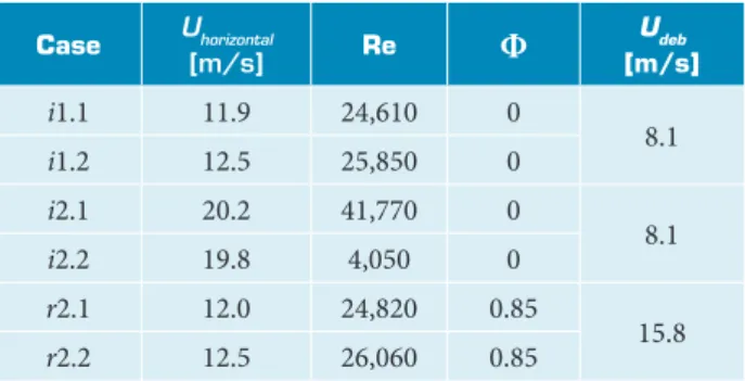
he numerical studies in this paper are compared with experimental results obtained from the ORACLES test rig (Besson 2002). The chosen experimental cases are shown in Table 1. The number after the dot refers to the upper inlet, named 1, and to the lower inlet, named 2. Uis the velocity measured on the x axis and “axial” concerns to this velocity measured in the half height of the respective inlet channel, in a position 170 mm far from the origin, indicated in Fig. 2. he equivalence ratio Φ is present in the reactive case
r2 and Udebrefers to the inlet average speed.
he inert case i1 has Reynolds numbers approximately the same of the ones obtained with the reactive r2 case, as it can be seen in Table 1. his correspondece is chosen purposely to test the turbulence model in this Reynolds range for i1 before test the combustion model coupled with the turbulence model in the case r2. he numerical schemes and k - ω conigurations are tested in higher Reynolds numbers by case i2.
Out of a large number of possible numerical schemes and combustion model conigurations, ive comparations are chosen in this paper, as shown in Table 2, with modiications in the temporal discretization scheme and divergence term discretization as well the used Ξ modelling. In the conigurations 3, 4 and 5 it is used a Linear Upwind scheme for velocity (U), pressure (p), kinetic energy (k) and speciic dissipation (ω) and Gauss Limited Linear for the other variables, whereas in the conigurations 1 and 2 the predominant divergence scheme
Figure 2. Sudden expansion detail. 29.9
130.6 70.4
30.4
30.4 14
o
29.9 x y z Figure 1. Fluid volume.
Figure 3. 2-D mesh detail.
Case Uhorizontal
[m/s] Re
Φ
U
deb
[m/s]
i1.1 11.9 24,610 0
8.1 i1.2 12.5 25,850 0
i2.1 20.2 41,770 0
8.1
i2.2 19.8 4,050 0
r2.1 12.0 24,820 0.85
15.8 r2.2 12.5 26,060 0.85
Table 1. Experimental cases for numeric comparison.
(11)
(12)
(13)
for all variables is the Gauss Limited Linear. he comparison between conigurations 4 and 5 leads to the analysis of the lame wrinkling model and, consequently, the lame shape and its characteristics.
BoundAry Conditions
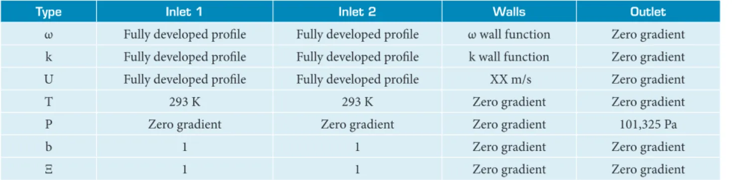
he outlet pressure condition is atmospheric, the walls are isolated, the inlet temperatures are setted as 293 K and b and Ξ are considered unitary in inlet. he mixture fractions follow Table 1 in inlets. he ignition points are equally spaced, located in x = 0.005 mm and away from horizontal walls 0.005 mm. he ignition time takes 0.05 s. Wall functions are used for ω and k, detailed in Menter (1994).
Table 3 shows the detailed boundary conditions chosen for the numerical simulation; notice that it is a bidimensional simulation. Fully developed proiles are imposed as initial conditions for k,
ωand U ields by mapping the results of simulations performed in the OpenFOAM standard solver BoundaryFOAM (ESI-Open CFD 2015). his is a one-dimensional steady-state OpenFOAM olver code to simulate fully developed turbulent lows.
RESULTS
inert CAsesIn Fig. 4, it is shown the velocity ield for case i2 using coniguration 1. A non-physical behavior is observed due the
Euler scheme use in the temporal term discretization, which creates an irreal wake in the inlet separating plate. he error is analyzed in Fig. 5, where it is shown the horizontal velocity proile at the origin. H is the backward step heigth and Udebis found in Table 2.
he wake is caused by the ampliication of the pressure difference between the two inlets and the profile for Euler scheme shown in Fig. 5 does not represents the reality.
type inlet 1 inlet 2 walls outlet
ω Fully developed proile Fully developed proile ω wall function Zero gradient
k Fully developed proile Fully developed proile k wall function Zero gradient
U Fully developed proile Fully developed proile XX m/s Zero gradient
T 293 K 293 K Zero gradient Zero gradient
P Zero gradient Zero gradient Zero gradient 101,325 Pa
b 1 1 Zero gradient Zero gradient
Ξ 1 1 Zero gradient Zero gradient
Table 3. Boundary conditions.
Coniguration temporal term divergence term Ξ model
1 (inert) Euler Gauss Limited Linear
-2 (inert) Backward Euler Gauss Limited Linear
-3 (inert) Backward Euler Linear Upwind
-4 (reactive) Backward Euler Linear Upwind Algebraic
5 (reactive) Backward Euler Linear Upwind Transport
Table 2. Numerical schemes and Ξ models.
Figure 4. Numeric error in the central wake using Euler scheme for temporal term.
Figure 5. Horizontal velocity proile in x = 0 for temporal schemes and experimental results.
Umean magnitude
10 20
22.53243 0
–1 0
0.2 0.6 1 1.4
1 2 3 4 5
Y/H
U/U
d
eb
Euler Scheme Backward Scheme
Figure 6. Mean velocity ield, streamlines and stations in
case i 2/coniguration 3.
Station 6
(9.7H)
Umeanmagnitude
Station 5 (6.35H) Station 4 (3.01H) Station 2
(0H)
20.0 10.0
x (m)
y (m) 0.00 21.1
–0.1 –0.2 –0.3 –0.065 0.065 H 0 0
0.1 0.2 0.3 0.4
Station 1 (–170 mm)
Station 3 0.33H)
Station 1 Station 2 Station 3 Station 4 Station 5 Station 6
Besson (2001) This work
10 14 18 22 0.6 1 1.4 –0.5 0.5 1.5 –0.5 0.5 1.5 –0.5 0.5 1.5 –0.5 0.5 1.5
U/U deb 0.2 1 2 3 3.5 2.5 5 4 3 2 1 5 4 3 2 1 5 4 3 2 1 5 4 3 2 1 1.5 0.5 Y/H Station 3 U/U d eb Station 4 U/U d eb Station 5 Y/H U/U d eb Besson (2001) This work –0.06 –0.04 –0.02 2 3 0 1 0.02 –0.15 –0.1
–0.025 2 3
0 1 0.05 4 5 –0.08 –0.04 2 3 0 1 0.04 4 5
Figure 7. Axial velocity proiles for stations in case i 2/coniguration 3.
Figure 8. Vertical velocity proiles in stations in case i 2.
he diference between conigurations 2 to 3 is just the numerical scheme for the divergence term, changed to LUDS. Both results do not show visible diference in the total results; however coniguration 3 converges in 0.7 s while coniguration 2 converges in 1.5 s. Considering these results coniguration 3 is the chosen for inert simulations.
Figure 6 shows the flow velocity field for i2 with flow streamlines. It can be seen in this same igure black vertical lines where the variables are analyzed and compared to experimental data, which are named as stations. By observing the lowield it can be noted an asymmetry between the upper and lower recirculation zone, as shown by Besson (2002). In Fig. 7 the numerical and experimental horizontal velocity proiles are compared for the stations shown in Fig. 6 and in Fig. 8 the vertical velocity proiles in the stations 3, 4 and 5 are shown. he weak agreement of the vertical velocity proiles in this comparison shows that the turbulence model is not able to capture the recirculation zones using low velocity luctuation levels but it provides very good agreement for horizontal velocity proiles.
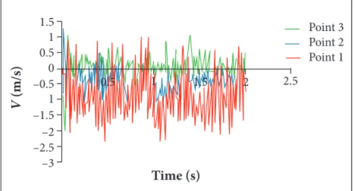
Figures 9 and 10 show the time history for, respectively, the vertical and horizontal velocities in three points in the
1.5 1 0.5 0 –0.5 1 –3 –2.5 –2
0.5 1 1.5 2 2.5
Point 3 Point 2 Point 1
–1.5
Time (s)
V
(m/s)
Y/H = –2
Y/H = 2
8
4
0
6 10 14 18
X/H V/U d eb 2 –8 –4 60 50 40 30 20
–10 0.5 1 1.5 2.5
Point 3 Point 2 Point 1 10 Time (s) U (m/s) Station 3
Station 5 Station 6
Station 4
–1 0 1 2
5
4
3
2
1
–1 0 1 2
5
4
3
2
1
–1 0 1 2
5
4
3
2
1
–0.5 0.5 1.5
5 4 3 2 1 Besson (2001) This work U/U deb U/U deb Y/H Y/H Y/H Station 4 U/U d eb U/U d eb Besson (2001) Present work –0.2 –0.15 –0.1
–0.05 1 2 3 4 5
0 0.05 0.01 Station 6 –0.02 –0.01 0.01 0 0.03 0.02 2
1 3 4 5
0.04 0.05 0.06 Figure 9. Vertical velocity luctuation in measuring points in
stations 3, 5 and 6.
Figure 11. Vertical velocity at 2H and -2H for case i 2. Figure 10. Horizontal velocity luctuation in measuring points in stations 3, 5 and 6.
Figure 12. Horizontal velocity proiles in case i 1.
In Fig. 11 it can be noted the average vertical velocity evolution along two horizontal lines, located in Y/H = –2 and Y/H = 2. The recirculation zones lenghts are defined where the velocity reverts the direction in these lines. This results agree with Abbott and Kline (1962), which measures the upper and lower recirculation zone lengths in a square profile duct with sudden expansion. For an expansion ratio of 1.8, approximately the value for ORACLES test rig, the author obtained the length of 10 H and 4 H. In this study these values are 12 H and 4 H, representing a good agreement.
Figure 13. Vertical velocity proiles in case i 1.
By analysing case i1 now, in a lower Reynolds range, the behavior for velocity ields is similar to i2, as presented in Fig. 12 for horizontal velocity proiles in stations 3, 4, 5 and 6. In Fig. 13 it is seen the vertical velocity proiles in stations 4 and 6 showing the turbulence model error in the capture of the recirculation zone in this low velocity level. In Fig. 14
Figure 15. Horizontal velocity proiles comparison in station 5. U/U
deb
Y/H
5
5
Algebraic
Experimental Transported Ξ 4
4 3
3 2
2 1
1 0
–1
290. 809 2149. 42 400 1200 1600 2000
T
Figure 16. Instantaneous temperature ield for case r2.
Figure 17. Flame front visualization in case r2.
Figure 18. Flame wrinkling in case r2.
temperature [K]
Case Numerical Experimental Diference
r2 2,149 2,103 2%
Table 4. Adiabatic lame temperature obtained through coniguration 5 and by Besson (2002).
k
m e a n
ω
m e a n
2 4
0
10000
1000 1e+5
222.018 183187
5.325807
Figure 14. k and ω ields for case i 1.
conditions used and visible asymmetry for case i1 in the same way as case i2.
reACtive CAse
With the same boundary conditions of the i 1 case, except the mass fraction boundary condition, case r 2 is the reactive case i1. Two configurations are tested, one of them with the algebraic flame wrinkling model and another using a transported model. To define the best configuration, velocity profiles comparison is conducted in the burned gas acceleration zone, where the stations 4, 5 and 6 are located.
In Fig. 15 it is shown a comparison between the algebraic model, transport model and experimental results, giving large advantage for transported model when defining the flame length and correct velocity fields. By this finding, configuration 5 is chosen for obtaining all the results for reactive simulation.
Figure 16 shows the temperature distribution for r2 case. In Figs. 17 and 18 the temperature field and a front flame photography taken during Besson (2002) i 2 experiment
are shown, respectively, pointing out the similitude with the numerical simulation.
U/U
deb
Y/H
Station 3 Station 4 Station 5
Besson (2001) Present work
5
4
3
2
2
–1 1 1 2 3
1
1 1.5
–0.5 0
0
5
4
3
2
1
5
4
3
2
1
Figure 19. Horizontal velocity proiles for case r2. Figure 20. Vertical velocity proiles for case r2.
U/U
d
eb
Besson (2001) Present work
–0.3 –0.1 –0.2 0.2
0
1 2 3 4 5
0.3
0.1
U/U
d
eb
–0.02 0.02 0.04
0
1 2 3 4 5
0.06
U/U
d
eb
–0.3 –0.05 0.15
0
1 2 3 4 5
0.25
Y/H
Abbott DE, Kline SJ (1962) Experimental investigations of subsonic turbulent low over single and double backward facing steps. J Basic Eng 84(3):317-325. doi: 10.1115/1.3657313
Besson M (2002) Étude experimentale d’une zone de combustion en écoulement turbulent stabilisee en aval d’un elargissement brusque symetrique (PhD thesis). Poitiers: Poitiers University.
Bilger R, Pope S, Bray K, Driscoll J (2005) Paradigms in turbulent
combustion research. P Combust Inst30(1):21-42. doi: 10.1016/
j.proci.2004.08.273
CFD-Online (2011) Weller test case for XiFoam: results discrepancy; [accessed 2015 Jun 1]. http://www.cfd-online.com/Forums/ openfoam/93198-weller-test-case-xifoam-results-discrepancy.html
Figures 19 and 20 show, respectively, the horizontal and vertical profiles in the same stations 3, 4 and 5 adopted for i2 simulations. In Fig. 19 it is shown a noteworthy concordance between the numerical and experimental results using configuration 5, detailed in Table 2. The best results for vertical velocity profiles in Fig. 20 are due to high burned gases velocity relative to the combustion phenomena.
DISCUSSION
In this study it is described the numerical simulation of some experiments carried out in the ORACLES test rig using b-Ξ lame wrinkling combustion model and SST k-ω turbulence
model focusing on the coupling adjustment between them. his experiment is particularly chalenging for numerical schemes testing due the pressure lutuations among the parallel inlet channels requiring special atention to the temporal discretization schemes. It should be noted that backward scheme for temporal term has reached the best results and maintains plausible behavior whereas the Euler scheme ampliies the pressure oscilations and
causes an irreal wake that starts in inlets separator blade. he results obtained from the reactive case show that the combination of the backwad Euler for temporal term and Linear Upwind for divergence terms is valid for reactive and inert lows in the Reynolds range tested in this study, and presents a better behavior than the inert case due the higher velocities. he transported Ξ model gives a large advantage for the reactive simulation where the algebraic model fails in determining correct velocity ields. With these results LES turbulence models associated with b-Ξ lame wrinkling combustion model can be used in the ORACLES test rig since there is a large database of temporal statistics available for this experiment.
openfoam.com
Gulder OL (1984) Correlations of laminar combustion data for alternative SI engine fuel. SAE Technical Paper.
Hirsch C (2007) Numerical computation of internal and external flows: the fundamental of Computational Fluid Dynamics. vol. 1. Oxford: Butterworth-Heinemann.
Jasak H (1996) Error analysis and estimation for the finite volume method with applications to fluid flows. London: University of London.
Kröger H, Hassel E, Kornev N, Wendig D (2010) LES of premixed flame propagation in a free straight vortex. Flow Turbul Combust 84(3):513-541. doi: 10.1007/s10494-009-9242-y
Law CK (2006) Combustion Physics. Cambridge: Cambridge
University Press.
Leoni EF (2010) Sviluppo di modelli di combustione turbolenta per fiamme diffusive (PhD thesis). Milan: Politecnico di Milano.
Lipatnikov A (2012) Fundamentals of premixed turbulent
combustion.Boca Raton: CRC Press.
Maas U, Pope SB (1992) Simplifying chemical kinetics: intrinsic low-dimensional manifolds in composition space. Combust Flame 88(3-4):239-264. doi: 10.1016/0010-2180(92)90034-M
Marble FE, Broadwell JE (1977) The coherent flame model for turbulent chemical reactions. DTIC Document.
Maric T, Hopken J, Mooney K (2014) The OpenFOAM technology primer. Germany: SourceFlux.
Menter FR (1994) Two-equation eddy-viscosity turbulence models for Engineering applications. AIAA J 32(8):1598-1605. doi: 10.2514/3.12149
Moriyoshi Y, Morikawa H, Kamimoto T, Hayashi T (1996)
charge conditions. SAE Technical Paper.
Moss JB (1980) Simultaneous measurements of concentration and velocity in an open premixed flame Combust Sci Technol 22(3-4): 119-129. doi: 10.1080/00102208008952377
Nguyen PD (2003) Contribution expérimentale à l’étude des
caractéristiques instationnaires des écoulements turbulents
réactifs prémélangés stabilisés en aval d’un élargissement brusque
symétrique (PhD thesis). Poitiers: Université de Poitiers.
Pitz RW (1981) An experimental study of combustion: the turbulent structure of a reacting shear layer formed at a rearward-facing step (PhD thesis). Berkeley: University of California.
Pope SB (1997) Computationally efficient implementation of combustion chemistry using in situ adaption tabulation. Combust
Theor Model1(1):41-63. doi: 10.1080/713665229
Qiao L, Dahm W, Faeth GM, Oran E (2008) Burning velocities and flammability limits of premixed methane air diluent flames in
microgravity. Proceedings of the 46th AIAA Aerospace Sciences
Meeting and Exhibit; Reno, USA.
Spalding D (1971) Mixing and chemical reaction in steady
confined turbulent flames. Proceedings of the 13rd International
Symposium on Combustion; Pittsburgh, USA.
Sweby PK (1984) High resolution schemes using lux limiters for hyperbolic conservation laws. SIAM J Numer Anal 21(5):995-1011.