The role of Twitter in the U.S. financial market

(1)

FUNDAÇÃO GETULIO VARGAS ESCOLA DE ECONOMIA DE SÃO PAULO

FERNANDO MARTINELLI RAMACCIOTTI

THE ROLE OF TWITTER IN THE U.S. FINANCIAL MARKET

SÃO PAULO 2018

(2)

Dissertação apresentada à Escola de Econo-mia de São Paulo como requisito à obtenção do título de Mestre em Economia

Área de concentração: Economia, Econometria

Orientador:

Prof. Dr. Bruno Cara Giovannetti

SÃO PAULO 2018

(3)

Ramacciotti, Fernando Martinelli.

The role of Twitter in the U.S. financial market / Fernando Martinelli Ramacciotti. - 2018.

48 p.

Orientador: Bruno Cara Giovannetti

Dissertação (MPFE) - Escola de Economia de São Paulo.

1. Redes sociais on-line. 2. Mídia social. 3. Mercado financeiro - Estados Unidos. 4. Comportamento Avaliação. I. Giovannetti, Bruno Cara. II. Dissertação (MPFE) -Escola de Economia de São Paulo. III. Título.

CDU 336.76::65.012.45(73)

Ficha catalográfica elaborada por: Raphael Figueiredo Xavier CRB SP-009987/O

(4)

Dissertação apresentada à Escola de Econo-mia de São Paulo como requisito à obtenção do título de Mestre em Economia

Área de concentração: Economia, Econometria

Data da aprovação: __/__/____

Banca Examinadora:

Prof. Dr. Bruno Cara Giovannetti EESP - FGV

Prof. Dr. Fernando Chague EESP - FGV

Prof. Dr. Rodrigo de Losso FEA - USP

SÃO PAULO 2018

(5)

Resumo

Eventos significativos no mercado financeiro ocorrem apenas se existe uma sintonia entre grupos de pessoas e a mídia é o principal meio para tal. Trabalhos anteriores encontraram relações entre notícias de jornais e o indicadores usados no mercado financeiro. Este trabalho, de certo modo, retoma as descobertas da literatura tradicional sobre a relação entre o comportamento de investidores do mercado financeiro e as notícias, porém agora no contexto da Era Moderna das mídias sociais. O principal objetivo desse estudo é identificar se o sentimento dos usuários do Twitter tem alguma relação com o mercado financeiro. Construiu-se uma base de dados que unifica dados não-estruturados de tweets com dados estruturados de séries de tempo financeiras do índice americano S&P500, o seu volume negociado e a sua volatilidade (esta medida pelo índice VIX). Os dados não-estruturados foram processados para poder categorizar cada palavra de cada tweet em categorias semânticas definidas dicionário psicológico Harvard-IV. Após isso, foram criados duas medidas de sentimento via Análise de Componentes Principais (PCA na sigla em inglês): os Fatores de Engajamento e Otimismo. Adotou-se o modelo de Vetor Autoregressivo (VAR) para estimar simultaneamente os efeitos dos sentimentos e variáveis do mercado financeiro uns nos outros. Os resultados indicam que os usuários do Twitter parecem ser mais responsivos aos eventos do mercado, ou seja, o sentimento produzido por seus tweets parecem ser reflexo de eventos financeiros e não têm poder preditivo.

Palavras-chave: Redes sociais on-line; mídia social; mercado financeiro - Estados Unidos; comportamento - avaliação

(6)

Abstract

Significant market events in the financial market will only occur if there is synchrony among large groups of people and the media is the main vehicle to it. Previous works could find some relationship between newspapers and financial market indicators. This work revisits, in some sense, the findings of the traditional literature on financial market investors’ behavior and its relationship to the news, but now in the Modern Era context of social media. The main goal of this work is to identify if the overall sentiment of Twitter users has some relationship with the financial market. We created a database that joins non-structured data from tweets and structured time series data related to the S&P500 index, its trading volume and implied volatility (measured by the VIX). The non-structured data was processed in order to categorize each word from each tweet into several semantic categories defined by the Harvard-IV psychological dictionary. Then, two sentiment indexes were created via Principal Component Analysis (PCA): Engagement Factor (EF) and Optimism Factor (OF). Using Vector Autoregressive (VAR) framework, we simultaneously estimated the effects of sentiment on financial market variables and vice versa. Our results indicate that Twitter users seem to respond to financial market events, i.e. their sentiment is a consequence of financial events and do not have predictive power.

Keywords: on-line social network; social media; financial market - United States; behavior - assessment

(7)

List of Figures

Figure 3.1 – Distribution of tweets over the years . . . 17

Figure 3.2 – No. of tweets per user . . . 18

Figure 3.3 – Intra-year seasonality patterns . . . 19

Figure 3.4 – Level value of S&P500, VIX and S&P500 trading volume . . . 19

Figure 4.1 – GI categories relative frequency over time . . . 22

Figure 4.2 – Visualization of the first two principal axis . . . 23

Figure 4.3 – Original data projected on the first two principal axis . . . 24

Figure A.1 – Residual diagnostic plots from Engagement Factor estimation . . . 46

Figure A.2 – Residual diagnostic plots from Optimism Factor estimation . . . 46

Figure A.3 – Residual diagnostic plots from Returns estimation . . . 47

Figure A.4 – Residual diagnostic plots from VIX estimation . . . 47

(8)

List of Tables

Table 3.1 – Descriptive monthly statistics of the Twitter dataset . . . 18

Table 3.2 – Descriptive statistics of financial data over the considered period . . . . 20

Table 4.1 – Correlation structure between selected GI categories . . . 23

Table 4.2 – PCA results . . . 23

Table 4.3 – Descriptive statistics factors . . . 24

Table 4.4 – Augmented Dickey-Fuller test statistics . . . 26

Table 4.5 – VAR order selection according to IC statistics for each VAR(p) . . . . . 27

Table 5.1 – Social Media factors estimates . . . 29

Table 5.2 – Market effects on social media sentiment . . . 30

Table B.1 – Properties of ACF and PACF . . . 43

(9)

1 Introduction

The field of behavioral economics aims to better understand the behaviors of economic agents in many typical day-to-day situations - it is interesting how this field relates to psychology. In fact, pioneer researchers from psychology, such as Kahneman and Tversky, demonstrated interesting findings in the 1970’s. They have shown in Tversky and Kahneman (1971) that people assume that a small sample is highly representative of the population and, therefore, make erroneous inference. In their future works, in Kahneman and Tversky (1973) and Tversky and Kahneman (1974), they discovered what is called

representativeness heuristic which people under uncertainty tend to find familiar patterns

to make, hence, biased, judgments based on that.

Surely, this findings could have interesting applications for investors, specially those who use news as their main source of information. Overconfident investor could overweight their private information about certain stocks with respect to public data. As demonstrated in Daniel, Hirshleifer and Subrahmanyam (1998), they update their beliefs asymmetrically, i.e. outcomes that comply with their previous belief increase their confidence, but those that do not decrease the confidence modestly.

Shiller (2000) argues that although the media vehicles - newspapers, magazines, TV, the Internet - are detached observers of the market, significant market events in the financial market, specially, will only occur if there is synchrony among large groups of people and the media is the vehicle to spread it. He also points out that the media urges to attract audiences (as it is its inherent objective) and they may reinforce ideas that are not supported by evidence, create debates on a variety of topics that would otherwise not be as attractive, comment on market events with the so called specialists or celebrities -i.e. media might act as speculative propagator.

Besides the speculative property of the media, Tetlock (2007) found that the overall pessimism of a financial-related column of the Wall Street Journal has some predictive power on daily stock returns as well as on trading volume. Moreover, Engelberg and Parsons (2011) found the relationship between local news coverage and trading volumes on local brokerage accounts. It is also supported in García (2013) that people are more sensitive during recession and, therefore, news have more predictive power on such periods.

It is clear that the behaviorists literature found compelling evidence that economic agents are not fully rational. With the advent of the Internet, information is more accessible than ever before and such biases can be, at least, further studied. It is interesting to notice that we can easily identify trending topics and how fast they spread and we can now easily quantify it. Asur and Huberman (2010) showed that box-offices revenues predictions

(12)

Chapter 1. Introduction 11

based on Twitter chatter outperform traditional market models. Choi and Varian (2012) studied how Google Trends, the trending keywords searched on Google’s search engine, can help to predict the present, or nowcasting. They found that the search trends can help predict automobile sales, unemployment claims, travel destination planing and consumer confidence. Bollen, Mao and Pepe (2011) could construct a sentiment index based on Twitter posts and how the audience respond to economical, political and cultural events.

This work revisits, in some sense, the findings of the traditional literature on investors behavior and its relationship to the news, but now in the Modern Era of social media context. The main goal of this work is to identify if the overall sentiment of Twitter users has some relationship with the financial market, such as returns, trading volume and volatility, or if the users comments are solely backward-looking and reflects the overall market events.

To construct a sentiment index from Twitter corpora, the General Inquirer software, a computer-assisted approach to analyze text content proposed by Stone et al. (1962), took care of semantic categorization of each word of each tweet, from March 2007 up to October 2017. Then, Principal Component Analysis (PCA) was carried out in order to extract the latent state of the content. The first principal component is interpreted as measure of overall engagement whilst the second is related to optimism, together they are responsible to 72.4% of the total variance. To relate them with the financial market of the United States, we collected data from the S&P500 index - which is composed by the 500 largest companies listed on the main stock exchanges and it is often referred as the gauge of the US Economy - and the VIX index, a volatility index that serve as a proxy for the volatility of the S&P500 index.

We estimate the effects of sentiment and financial market variables on each other using a Vector Autoregressive (VAR) framework. Such model enables all the variables to be seen as endogenous and estimate the effects on each other separately. The variables used were Engagement Factor (scores from the first principal component), Optimism Factor (score from the second principal component), excess of returns of the S&P500 with respect to the 3-month Treasury Bill yield, on daily frequency, the trading volume of the S&P500 volume and the VIX index. We found that the impacts of the market changes are higher on the sentiment index than the opposite. This strongly supports that the social media reflects market events as opposed to be the drivers of them.

We found that a one-standard deviation impact on the overall engagement of Twitter users predicts a decrease of 0.1 basis point on return on the very next day. This could be related to the euphoria of the public that on average might drive people to irrational decisions in terms of investments. This hypothesis is even more compelling when we find that such increase in excitement is translated to 0.3% more volatility in the very next day as well. Optimism, on the other hand, seems only to influence trading volume

(13)

Chapter 1. Introduction 12

and in an interesting fashion: an increase in one standard deviation in optimism today predicts 0.8% more volume two days in advance. However, in we analyze the fourth lag, the sign is flipped, i.e. the impact of an increase in the optimism factor predicts that the volume will decrease 1% four days later.

The market variables impact on sentiment factors is more distributed over time lags. A one-percent increase in returns positively impacts the optimism factor in the very next day by 0.07 standard deviation, but has negative impact of 0.3 standard deviation four days after - this may be related to short memory. Moreover, a one-percent increase in returns accounts to almost 0.1 standard deviation of optimism on of the day after the next day. Trading volume affects the next day both on engagement and optimism, 0.14 and 0.04 standard deviation, but regarding optimism it also affects the day after the next day by 0.1 standard deviation as well. Volatility change seems to account to more impact in terms of magnitude: it positively correlates to engagement factor of the very next day by a ratio of one-percent to 0.2 standard deviation and on the two days after for optimism by a ratio of one-percent to 0.1 standard deviation. At 10% significance level, we have evidence that a one-percent change in the volatility negatively impacts 0.7 standard deviation on engagement factor one week after.

It is also true that the S&P500 index is composed by big companies that may be more resilient on the speculative nature of social media in the sense that social media may not bring new information that could fundamentally change the track of those companies stock prices. In that way, we could not find enough evidence that the sentiment on Twitter could drive or predict prices of such companies. On future works, however, it would be interesting to study the relationship between sentiment and smaller companies.

This work is organized as follows: chapter 2 reviews the behavioral economics literature as well as related works on media and financial market; chapter 3 describes the data collection method and descriptive statistics of them; chapter 4 provides the data preparation and the model used; chapter 5 contains an analysis of the results obtained; chapter 6 proposes a final reflection and grounds for extensions of this work. A brief theory review on PCA and Time series can be found in Appendix A and Appendix B, respectively. All the analysis and statistical modelling were done using open source tools such as Python and R programming languages and source codes can be found in

(14)

13

2 Literature Review

Investors have always wanted to understand better how the financial markets move and, if possible, predict the next move so that they can build their optimal portfolio. Since the investor plays a essential role when it comes to investing, the area of behavioral finance has been trying to correlate investors sentiment and behavior to the financial market. A great summary of behavioral economics and its application can be found in DellaVigna (2007).

2.1 Psychology

Psychological findings play an important role in behavioral economics. The so called

Law of small numbers was first shown by Tversky and Kahneman (1971) - people tend

to assume that a small random sample drawn from a population is highly representative. Therefore, when making prediction under uncertainty this erroneous inference can lead to systematic errors. They also showed that people tend to overweight recent and salient piece of information with respect to prior beliefs. Also, under uncertainty, people tend to make judgments by looking at familiar patterns being confident about its high representativeness in the population - an anomaly called representativeness heuristic in Kahneman and Tversky (1973), Tversky and Kahneman (1974).

A formal approach, using Bayesian inference, to model the inference by the law of small numbers was presented in Rabin (2002). It is assumed that each information that a person receives, call it a signal, is drawn from a urn of N < ∞ elements without replacement. Therefore, the smaller N , the more believer in the law of small number the person is. An example of how this works is the classical coin flip experiment. For instance, a person might prior believes that if a given coin is fair, then each pair of flips the number of heads must be equal to the number of tails. So, if he observes two heads in a row he might believe that the coin is biased. The same framework would apply for anything else, say security analysts forecasts, stock prices changes and so on.

Investor psychology is modeled on psychological grounds in Barberis, Shleifer and Vishny (1998). They assume that the earnings of an asset follows a random walk, but the investor does not know it and. Rather, he believes they switch between two possible states: mean-reversion and trend. On top of it, the transition rules, or probabilities, are fixed in his mind: for any given period, firm’s earnings are inertial, i.e. they tend to remain in their current state than switching. So, the investor look at firm’s earning at each period and updates his belief about the state in a Bayesian fashion. Conservatism and representativeness heuristics, which are psychological findings, both play roles while

(15)

Chapter 2. Literature Review 14

updating the investor beliefs. The first suggests that people are slow to change their opinions and it takes some time, and evidence, to an investor change their belief of which state the firm’s earnings are in. The latter helps to explain that people tend to see familiar patterns where they might not exist. In this case, if the earnings follow a truly random walk, a sequence of positive earnings might happens only due to chance, but for the investor it might resemble a positive trend pattern.

Another theory involving psychological evidence is suggested in Daniel, Hirshleifer and Subrahmanyam (1998), where investor overconfidence is explored. An overconfident investor will likely overweights the precision of his private information and underestimate the publicly available data. Such behavior will cause the stock price to overreact and the price will move to the full information move over the subsequent dates, as publicly information arises. The investor also asymmetrically updated their confidence observing the outcomes - if the publicly signal confirms their trading signal, then he becomes more confident, but if it is not confirmed, then confidence falls modestly.

2.2 Sentiment index

The overall attitude of investor towards the financial market is what we will call the investor sentiment. Some papers showed that the discounts of closed-end funds are correlated with sentiment index as shown in Lee, Shleifer and Thaler (1991) and Chopra et al. (1993) - actually they argue that closed-end fund discount rate are a measure of sentiment index. Neal and Wheatley (1998) take measures of sentiment index and test their ability to predict companies’ financial returns. Among other findings, they found a positive relation between closed-end fund discounts and small companies expected returns, but no relation with large firms. This is consistent, since most at the time of the study, most small firm stocks were held by individual investors and institutions held the large firm stocks (see Lee, Shleifer and Thaler (1991)). Otoo et al. (1999) studied the positive correlation between consumer sentiment and stock prices and raised a question about which one is the cause of the other. With individual data from a Michigan survey, they concluded that people tend to use the stock prices movement as a leading indicator of the future instead of consumer sentiment primarily influences stock prices.

2.3 Media influence

It is natural to assume that media is used by investor so that can track their investments performance (such as stock prices) and be informed about new events that might affect their portfolio. Tetlock (2007) measured how a popular Wall Street Journal column correlates with the financial stock market. The words from the column were extracted and categorized into 77 categories predetermined by a psychological dictionary.

(16)

Since a word can belong to several categories, a principal components analysis (PCA) was employed to keep the most important component of the the variance-covariance matrix of the word categories. The resultant factor was called the Pessimism Media Factor. A vector autoregressive (VAR) model was used to estimate the links between such media factor and the stock market. High levels of pessimism predicts downward pressure on prices. Moreover, high or low levels of pessimism factor are followed by high trading volume. Finally, to close the cycle, low returns lead to high levels of pessimism.

Similarly, García (2013) analyzed the effects of two columns from the New York

Time on the financial market. It is important to notice that these columns are are viewed

as description about recent market performance and speculation about its near future and not new piece of information. As Tetlock (2007), he also find that trade volume is predicted by extreme content, either positive or negative, providing additional evidence that traders are not fully rational. If they were so, and symmetrically informed, a publicly signal such as a newspaper column should not affect trading volume. The novel finding of the paper is that people tend to be more sensitive during recession and, therefore, the predictability power of the news content is much higher during economic downturns.

What if the same information event is covered by different media content sources? Engelberg and Parsons (2011) studied the effect of local media coverage on local brokerage accounts, from 1991 to 1996, a pre-Internet period. The main finding is that if the earnings announcement for a given S&P 500 firm is locally covered or not strongly influence the firm’s local trading, controlling for all fixed effects (e.g. firm-city closeness, timezones that might affect publishing date). The trading volume increases from 8% up to 50%. The evidence, however, supports prediction power from media coverage on trading volume only for trading volume on the same day that the coverage occurs. Moreover, they found that the local media coverage predicts trading only for day 1, i.e. the first possible day that the coverage can occur. For coverage initiated on future possible dates, there is no evidence of predictability.

Shiller (2000) describes how the media can relate to the financial market. The author argues that the media can actively drive public attention and they can support speculative price movements while they put their efforts to make news interesting to their audience.

2.4 Digital Era

The Internet today can serve as the main source of information, specially when it comes to news. Microblogging on Twitter, for instance, has become more popular and widely used as a channel to spread news. Bollen, Mao and Pepe (2011) studied how textual analysis on posts from from Twtitter users, or tweets, measures the public mood and how

(17)

it responds to social, political, economical and cultural events on the short term. Bollen, Mao and Zeng (2011) also carried a textual analysis from twitters and found that some

Calm and Happiness moods can predict the value of the Down Jones Industrial Average (DJIA). In fact, they are Granger causative of the value of the DJIA for a period of 3 to 4

days.

2.5 Other related work

Monetary policy and market sentiment has been explored by Chague et al. (2015). The paper has also conducted a textual analysis, but now from the Brazilian Central Bank’s Monetary Policy Committee press releases. Similarly to Tetlock (2007), they used PCA to build a measure of the communication sentiment, the Optimism Factor of the policy makers. They found that when policy makers are more optimistic, the long-term future interest rates drops. However, when Optimism is rather low, the market expectations responds with higher volatility on future interest rate.

Also related to monetary policy, Kurov (2010) found that the effects of monetary policy changes on the United States depends on market sentiment. Essentially, the study found that monetary policy changes in bull markets have little effect on stock returns and investor sentiment, but large effects in bear markets.

(18)

17

3 Data

The dataset studied is composed by social media posts on Twitter1 _{(or tweets), the}

S&P500 index and the VIX index. We can, therefore, split our datasets into non-structured and strucured data. The former is the textual data from tweets that needs to be processed somehow in order to fit any statistical and mathematical model. The latter is viewed and the historical time series of the financial data. We here just describe the raw data and further data preparation in order to ensure interpretable meanings and be corrected specified for our models is presented in ??

3.1 Non-structured data

Twitter was founded in 2006 and has increased popularity ever since, specially when it comes to news. Tweets can now be seen as a newsfeed and is often used as a source of trending topics. Therefore, the motivation to relate its data to the financial is straightforward.

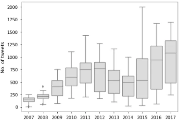
Figure 3.1 – Distribution of tweets over the years

(a) Number of tweets over the years (b) Tweets distribution over the years

We collected a variety of tweets that might be in the light of financial market practitioners. Our dataset has 495,259 tweets, from March 21, 2007 to October 31, 2017. Our sample was collected by filtering posts with at least one of the following keywords related to the US market: NASDAQ, NYSE, Dow Jones Industrial Average and Financial

Market. On top of it, we also collected tweets from the official accounts of the main

financial news sources of the US, such as Wall Street Journal, Financial Times Finance

News, CNBC, NY Times Business. Note that both collections methods are not mutually

exclusive, so we had to ensure uniqueness by dropping duplicates. However, one or more

(19)

Chapter 3. Data 18

users can post exactly the same tweet or even retweet it (i.e. reproduce someone’s tweet referencing the source). Thus, our tweets are unique per user and we do want to have duplicated tweets from different accounts as this may be a sign of a trending topic.

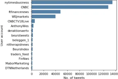
Figure 3.1 depicts the evolution of the number of tweets per year. We can clearly see that at the beginning, years of 2007 and 2008, the numbers of tweets are much smaller than in the following years. For some reason, the number of tweets in our sample decreased after 2011, but began increasing again in 2015 and kept like this ever since. Table 3.1 contains the descriptive statistics of each year. We can also clearly see that the news providers dominate our sample, NY Times and CBNC being the most active accounts, as depicted in Figure 3.2.

Table 3.1 – Descriptive monthly statistics of the Twitter dataset

Year N Monthly Avg St. Dev. Min Max

2007 10,123 1,012.3 237.5 412 1,254 2008 17,196 1,433.0 215.5 845 1,645 2009 32,663 2,721.9 634.3 1,647 3,479 2010 50,105 4,175.4 868.9 3,092 5,566 2011 59,423 4,951.9 862.1 3,634 7,080 2012 55,160 4,596.7 831.2 2,576 5,841 2013 45,745 3,812.1 1,025.4 2,438 6,322 2014 36,009 3,000.8 1,284.3 708 4,526 2015 52,566 4,380.5 2,498.0 664 7,650 2016 67,655 5,637.9 2,331.3 988 7,568 2017 68,614 6,861.4 1,213.2 4,192 8,573

Regarding seasonality, it is possible to notice that users are less active on the weekends. It seems reasonable, since we are taking samples related to the financial market and it is closed during weekends. When we look for monthly seasonality, however, there is no apparent distinction on users activity, as depicted in Figure 3.3.

(20)

Figure 3.3 – Intra-year seasonality patterns

(a) Tweets distribution by month (b) Tweets distribution by weekday

3.2 Structured data

The financial data collected is composed by daily adjusted closing price and volume of the S&P500 index2 _{and daily values of the VIX index}3_{, taken from Yahoo Finance}4_{, for}

the same period as the tweets collected, i.e. from March 21, 2007 to October 31, 2017 - a total of 2,651 samples (or business working days).

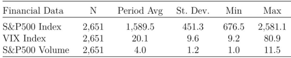
The S&P500 is traditionally used as indicator of the US economy, since it is a weighted composite of the 500 largest company by market capitalization. The VIX index is a measure of the implied volatility of the S&P500. Since it measures volatility, it is associated with uncertainty of the markets, i.e. periods with great volatility are, in general, when people are more risk averse. A summary can be found on Table 3.2.

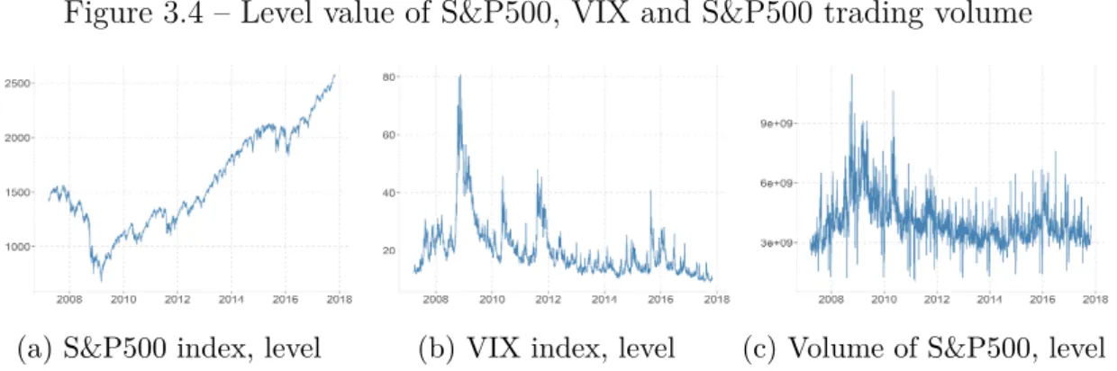
Figure 3.4 – Level value of S&P500, VIX and S&P500 trading volume

(a) S&P500 index, level (b) VIX index, level (c) Volume of S&P500, level

The S&P500 index increased by 79.5% over the period considered. It is interesting to notice that during the Financial Crisis of 2008-09, the S&P500 level dropped considerably. In fact, as depicted in Figure 3.4, it decreased by 53% between the beginning of 2008 and the bottom-most level in 2009 (March 9, 2009). The VIX level in such period also have

2 _{<https://us.spindices.com/indices/equity/sp-500>} 3 _{<http://www.cboe.com/vix>}

(21)

increased by 114% (i.e. from 23.2 up to 49.7), although it has peaked up to a level of 80 slightly afterwards. Trading volume of S&P500 is also affected by volatile periods.

Table 3.2 – Descriptive statistics of financial data over the considered period

Financial Data N Period Avg St. Dev. Min Max S&P500 Index 2,651 1,589.5 451.3 676.5 2,581.1

VIX Index 2,651 20.1 9.6 9.2 80.9

S&P500 Volume 2,651 4.0 1.2 1.0 11.5

(22)

21

4 Methodology and model

In this chapter, we describe our research methodology and the model used to analyze the data. However, data cleansing and preparation is needed to ensure interpretable and consistent results.

4.1 Data Preparation

Our goal is to have a sentiment index given by our Twitter dataset, specified in section 3.1 and, as already pointed out, we need to process such textual data. We used a dictionary approach to classify, measure and create a sentiment index of our tweets, similarly to what was done by Chague et al. (2015) and Tetlock (2007). Regarding our structured data, presented on section 3.2, we manipulated our historical series in order to ensure stationarity and also give them interpretable meaning. The following subsections discuss the procedures taken.

4.1.1 General Inquirer

The General Inquirer (GI), first introduced by Stone et al. (1962), is a computer-assisted system for content analysis which uses dictionaries lookups for word categorization and can also handle disambiguation. Today, the distributed software has two built-in psychological dictionaries, Harvard-IV and Lasswell, that maps thousands of words into 182 semantic groups, such as Negative, Positive, Pleasure, Passive, Power and so on. It is worth noticing the the categories are not mutually exclusive, i.e. one word can belong to more than one category. Also, one word alone can have multiple meanings that is given by the context and each one of possible meanings can belong to different categories - that is why disambiguation plays an essential role.

The software analyzes each word of our corpora and map them into one of the categories of the dictionary and the output is given in both the absolute and relative frequency of words in each category. We have grouped the tweets on a daily basis, generating one file per day with all the posts of the corresponding day and then passed all the files to the GI software. Finally, we can have a quantifiable meaning for our textual data.

4.1.2 Latent sentiment

Similarly to the approaches in Chague et al. (2015) and Tetlock (2007), we carry a Principal Component Analysis (PCA) in order to extract the latent sentiment of our sample of tweets already categorized by the GI. The PCA technique aims dimensionality

(23)

Chapter 4. Methodology and model 22

reduction by finding orthogonal vectors that captures the variance of the original data and are a linear combination of the original variables. A formal definition is found in Appendix A.

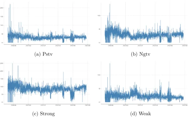
For simplicity sake, we studied just the four main categories of the Harvard-IV dictionary: (i) Pstv, related to positive words; (ii) Ngtv, related to negative words; (iii)

Strong, related to word that show strength, power, control, authority, etc.; and (iv) Weak, related to words that show weakness, submission, dependence, vulnerability, etc. In

Figure 4.3 we can see how each category evolves over time and in Table 4.1 we can see there is no pair of variables with more than 40% of correlation, which is good since we want to avoid redundant variables (i.e. highly correlated).

Remember that Figure 3.1 showed a growth tendency in the number of tweets in our dataset. It is straightforward to realize that the absolute frequency of each GI category will also follow such trend. Therefore, we used the relative frequency to avoid feed our PCA algorithm with the trend of our number of tweets. Also, before carry a PCA, we also scaled (to zero mean and unit variance) our GI output so that none of the categories’ variance prevails over the other (see Appendix A).

Figure 4.1 – GI categories relative frequency over time

(a) Pstv (b) Ngtv

(c) Strong (d) Weak

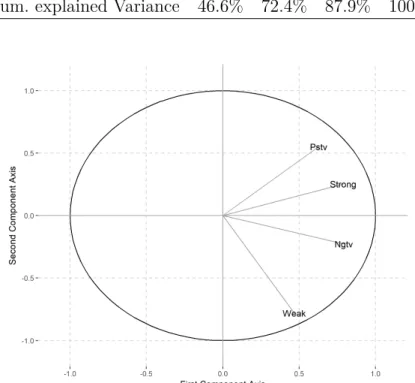
After running a PCA, we could reduce our dimension from 4 to 2, capturing 72.4% of the original variance. Table 4.2 summarizes the PCA results, giving the loading coefficients, associated eigenvalue λ and the variance explained. The first principal component, namely

P C1 has all its coefficients greater than zero and there is not a coefficient that strong

dominates the others - we could interpret this component as the Engagement of Twitter users. Now the second component assigns positive weights to Pstv and Strong categories,

(24)

Table 4.1 – Correlation structure between selected GI categories

Pstv Ngtv Strong Weak Pstv 1.00

Ngtv 0.26 1.00

Strong 0.40 0.46 1.00

Weak 0.03 0.34 0.14 1.00

but negative to Ngtv and Weak - since they are opposite pairs of categories and there is positive weight to positive categories, we interpret it as a measure of Optimism. From Figure 4.2 it is clear the cluster as a result of the second principal axis.

Table 4.2 – PCA results

GI category PC1 PC2 PC3 PC4 Pstv .46 .54 .67 .20 Ngtv .58 −.22 −.41 .66 Strong .58 .25 −.40 −.67 Weak .34 −.77 .47 −.27 λ 1.86 1.03 .62 .48

Cum. explained Variance 46.6% 72.4% 87.9% 100%

Figure 4.2 – Visualization of the first two principal axis

We need now to project our original data into this new coordinate system formed by the first two components:

(25)

where X is our (N × p) original scaled data, wi the (p × 1) loading vector associated with

the i-th principal component and ti is defined as the (centered) score, or the projected data,

into the i-th principal axis, of size (N × 1) (see Appendix A). In our case, p = 4 categories and N = 3, 878 is the length of our tweets dataset, resampled on a daily frequency.

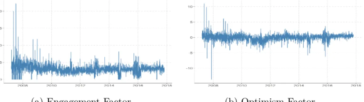
Note, again, that since we will use only 2 principal components to project our data, we reduced our original dataset X of size (N × 4) to our score matrix T of size (N × 2), as T = [t1 t2]. Since t1 contains the original data projected on the principal axis related

to Engagement, we called those scores Engagement Factor (EF ), and the t2 scores form

the Optimism Factor (OF ). Their evolution over the considered period can be seen in Figure 4.3 and its statistics in Table 4.3.

Figure 4.3 – Original data projected on the first two principal axis

(a) Engagement Factor (b) Optimism Factor

Table 4.3 – Descriptive statistics factors

Factor N Period Avg St. Dev. Min Max

EF 3,878 0.0 1.37 −5.50 7.09

OF 3,878 0.0 1.01 −13.64 11.0

It is interesting to note how the loadings we get differ from the one in Chague et al. (2015) and Tetlock (2007), where the principal axis obtained already relate to optimism or

pessimism. This was expected, since the corpora analyzed in those studies were Central Bank communication reports and columns from a newspaper, respectively in Chague et al. (2015) and Tetlock (2007). With that, it is reasonable to assume that a specific columns

on a given day will have a latent sentiment towards the view of the author as well as the Central Banks reports will need to address monetary policy perspectives that carry an inherent sentiment. When we analyze thousands of tweets per day, we capture the overall sentiment since there are lots of people with different opinions expressing different sentiments about the current scenario. Thus, an overall engagement of the people is the element with the highest variance.

(26)

4.1.3 Time series

We now have structured and non-structured data as time series format. However, before proceed to the modelling phase, we need to ensure stationarity so that our model is consistent.

A time series is weakly stationary if it has time invariant components up to the second moment. Although there are more ways of stationarity, from now on we will omit the term weak(ly) from weakly stationary time series and when we say that a series is stationary or not, we are referring to weak stationarity. Such kind of stationarity is usually enough to most models, specially the one we will use. Formal statistical tests provide a useful method to check whether a time series has a unit root or not, i.e. if it is an Integrated

Process. In fact, an integrated process of order d, i.e. I(d) has d unit roots and needs to be

differenced d times to become stationary. Additionally to such unit root tests, analyzing the Autocorrelation and Partial Autocorrelation Functions (ACF and PACF, respectively) is very insightful (see Appendix B for a time series review).

In general, for financial data the level value does not provide meaningful interpre-tation and we usually are interested in the change of such variables. For indexes and stock prices, the percentage change is a measure of return, defined as:

Rt= Pt Pt−1

− 1, (4.2)

where Rt is the return over the period [t − 1, t] and Pt is the level value (e.g. price of

stocks) at time t. It is also usual to express the log returns:

rt = log (Pt) − log (Pt−1) = pt− pt−1, (4.3)

where log X is the natural logarithm of X. The lowercase notation, such as rt or pt, is

defined as the logarithm of the level value, e.g. pt= log (Pt) and rt= log (Rt).

Also, it is usual to express return of a financial asset as the excess return with respect to a risk-free investment. In the case of the US market, it is common to use the yield of the 3-month US Treasury Bill as a proxy for the risk free rate in the United States. Therefore, we define the excess of return rxs

t of a financial asset as:

r_txs= rt− rtf, (4.4)

where rxs

t denotes the excess ("xs") of returns of a financial asset rt with respect to the

return of a risk-free investment rf_t, the yield of 3-month US Treasury Bills in our case, provided by the US Treasury1_.

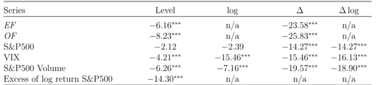
In Table 4.4 we can see the test statistics for the Augmented Dickey-Fuller, with null hypothesis that the series has unit root and the alternative is that it is stationary. It

(27)

was filled by "n/a" where a series transformation is either not applicable or does not make economic sense. For instance, the EF and OF factors have negative and zero values, where the log is not defined. Also, for the excess of log return series, it does make sense to apply logarithm again and its first difference would be an uncommon measure of the acceleration of the S&P500 level. The test was done for the series in level, log transformed and first difference of the log. Note that the first difference of the log of the level of S&P500 is the same as the log return of the S&P500 and the level of the excess of return of the S&P500 is useful only on the level and log, since it is already a differenced series. Although the level of VIX and S&P500 are stationary, we prefer to use its first differenced of log, since it provides a measure of percentage change. Note that S&P500 is not stationary at the level and log, as expected, since in Figure 3.4 we see a clearly upward trend over the years, but when differenced it becomes stationary as well as the excess of return series. Despite the peaks of VIX and S&P500 Volumes, they can be considered stationary even at the level. Both created factors, EF and OF are also stationary.

Table 4.4 – Augmented Dickey-Fuller test statistics

Series Level log ∆ ∆ log

EF −6.16∗∗∗ _n/a _−23.58∗∗∗ _n/a

OF −8.23∗∗∗ _n/a _−25.83∗∗∗ _n/a

S&P500 −2.12 −2.39 −14.27∗∗∗ _−14.27∗∗∗

VIX −4.21∗∗∗ _−15.46∗∗∗ _−15.46∗∗∗ _−16.13∗∗∗

S&P500 Volume −6.26∗∗∗ _−7.16∗∗∗ _−19.57∗∗∗ _−18.90∗∗∗

Excess of log return S&P500 −14.30∗∗∗ _n/a _n/a _n/a

Note: ∗p<0.1;∗∗p<0.05;∗∗∗p<0.01

log is the the log transformed series and ∆ means the first difference

The series we propose to work on are, therefore, the factors EF and OF , obviously, in addition to the first difference of the VIX and S&P500 Volume and the excess of return of the S&P500. The reason to choose the first difference of the log for the VIX and Volume, in spite of their stationarity behavior on the level, is because it can be thought as a rate of change and, thus, easier to interpret. The choice to work with level of EF and OF is because they are stationary at level and their intuition are hard enough to grasp at level that taking a transformed series would make it even harder.

4.2 Model

In our model, we simultaneously estimate the relationships among returns, sentiment and volume. A model that allow this kind of structure is a VAR (Vector Autoregressive) model, see Box et al. (2015), Durbin and Koopman (2012), Enders (2014) and Lütkepohl (2005).

(28)

A VAR of order p, i.e. VAR(p), is modeled as (see Appendix B):

Φ(L)Xt= c + εt, (4.5)

where Xt = (x1t, . . . , xnt)0 is an (n × 1) vector with n time series variables, L is the lag

operator such that Lk_x

t = xt−k, Φ(L) = In− A1L − . . . − ApLp is the lag polynomial

where each Ai is an (n × n) coefficient matrix, c is an (n × 1) constant vector and εt is an

(n × 1) vector of unobservable zero-mean white noise process. In our model we have:

Xt =            EFt OFt Rett ∆Vlmt ∆Vixt            , (4.6)

where EFt is the Engagement Factor (i.e. the scores of the first principal component), OFt

is the Optimism Factor (i.e. the scores of the second principal component), Rett is the

excess of return of the S&P500 calculated as described in Equation 4.3, ∆Vlmt is defined

as the first difference of the log of the S&P500 trading volume and ∆Vixt is defined as the

first difference of the log of the VIX index. As tested in subsection 4.1.3, all of these time series are stationary and, thus, the roots of the lag polynomial Φ(L) from Equation 4.5 lie outside the unit circle and, hence, the our VAR model is stable (see section B.7 from Appendix B).

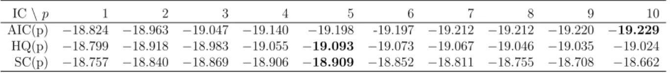
The only parameter that is left to define is the order p of our VAR model. In order to estimate it, we estimated multiple multiples, up to the lag p = 10 and check which model order is the most informative, measured by information criteria (IC) statistics. From Table 4.5 we would choose the order p = 10, p = 5 and p = 5 according to Akaike Information Criteria (AIC), Hannan-Quinn (HQ) and Schwarz Criterion (SC), respectively. We choose p = 5, since it is more intuitive to analyze effects lasting the equivalent of a business week (5 business day in a week). At this point, it is worth noticing that since we are merging all time series, we chose to drop weekends and holidays that were presented in the Twitter dataset but not in the financial data, remaining with a total of 2,646 samples.

Table 4.5 – VAR order selection according to IC statistics for each VAR(p)

IC \ p 1 2 3 4 5 6 7 8 9 10

AIC(p) −18.824 −18.963 −19.047 −19.140 −19.198 -19.197 −19.212 −19.212 −19.220 −19.229 HQ(p) −18.799 −18.918 −18.983 −19.055 −19.093 −19.073 −19.067 −19.046 −19.035 −19.024 SC(p) −18.757 −18.840 −18.869 −18.906 −18.909 −18.852 −18.811 −18.755 −18.708 −18.662

Each equation of our VAR model can be thought as a standard regression and can be estimated by OLS (ordinary least squares). Our model equations are represented as

(29)

follows:

EFt= c1+ α1L1−5(EFt) + β1L1−5(OFt) + γ1L1−5(Rett) + η1L1−5(∆Vlmt)

+ θ1L1−5(∆Vixt) + ε1,t (4.7)

OFt= c2+ α2L1−5(EFt) + β2L1−5(OFt) + γ2L1−5(Rett) + η2L1−5(∆Vlmt)

+ θ2L1−5(∆Vixt) + ε2,t (4.8)

Rett= c3+ α3L1−5(EFt) + β3L1−5(OFt) + γ3L1−5(Rett) + η3L1−5(∆Vlmt)

+ θ3L1−5(∆Vixt) + ε3,t (4.9)

∆Vlmt= c4+ α4L1−5(EFt) + β4L1−5(OFt) + γ4L1−5(Rett) + η4L1−5(∆Vlmt)

+ θ4L1−5(∆Vixt) + ε4,t (4.10)

∆Vixt= c5+ α5L1−5(EFt) + β5L1−5(OFt) + γ5L1−5(Rett) + η5L1−5(∆Vlmt)

+ θ5L1−5(∆Vixt) + ε5,t (4.11)

where the operator L1−5(.) = (L + . . . + L5)(.) is defined here as the lag operator from 1

to 5, ci and εi the constants of the vectors ct and εt from Equation 4.5, αi, βi, γi, ηi and

θi are (1 × 5) vectors composed by the coefficients of each lag of the series of Xt and part

(30)

29

5 Results

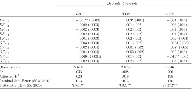
Since we are primarily interested in the social media impact on the financial market, we begin by assessing the coefficients related to the media factors, i.e. αi, βi from

Equation 4.9, Equation 4.10 and Equation 4.11. Then we inspect the responsiveness of the social media with respect to market events, i.e. Equation 4.7 and Equation 4.8. The complete estimates from all equations of our model can be found in Table A.1.

It is interesting to note from our estimates from Table 5.1 the overall engagement tested significant from its immediate effect on the next days’ excess of return of the S&P500 index. At 5% significance level, the impact of a one standard deviation change in the engagement factor is a negatively impacts 0.1 basis point in next day’s S&500 excess of returns and 0.3 basis point, at 10% level, the VIX index, where 1 basis point is equivalent to 0.01%. All the other previous days of the engagement and optimism factors have statistical zero impact on returns and VIX. However, previous engagement and optimism factor affect the next day’s respective factor, i.e. a positive change on today’s engagement increases future engagements up to a week.

Table 5.1 – Social Media factors estimates

Dependent variable: Ret ∆Vix ∆Vlm EFt−1 −.001∗∗(.0003) .003∗(.002) −.004 (.004) EFt−2 .0002 (.0003) .001 (.002) −.006 (.004) EFt−3 −.0002 (.0003) .002 (.002) .001 (.004) EFt−4 −.0002 (.0003) −.002 (.002) .001 (.004) EFt−5 .0001 (.0003) −.002 (.002) .006∗(.004) OFt−1 .0003 (.0003) .001 (.002) .0003 (.005) OFt−2 −.0002 (.0004) .0001 (.002) .008∗(.005) OFt−3 .0004 (.0004) −.0005 (.002) .002 (.005) OFt−4 .00004 (.0004) .001 (.002) −.010∗∗ (.005) OFt−5 .0002 (.0003) .002 (.002) .005 (.005) Observations 2,646 2,646 2,646 R2 _.033 _.028 _.206 Adjusted R2 _.023 _.019 _.198 Residual Std. Error (df = 2620) .013 .073 .170 F Statistic (df = 25; 2620) 3.544∗∗∗ _3.023∗∗∗ _27.172∗∗∗ Note: ∗_p<0.1;∗∗_p<0.05;∗∗∗_p<0.01

Standard deviations in parenthesis

When we analyze the trading volume, we can only reject the null hypothesis for the previous week’s engagement and both lags 2 and 4 for the optimism. To summarize, a one-standard deviation change in the engagement factor increases 0.6 basis points the next week’s S&P500 trading volume. A one-standard deviation change in optimism, on the other hand, increases trading volume by 0.8 basis point with a two-day delay, but

(31)

Chapter 5. Results 30

subsequently decreases 1 basis point (the 4th lag impact). This is consistent to what was studied in Tetlock (2007), where a positive change in the pessimism factor (or a decrease in optimism) first increases volume due to a group of liquidity traders, but the equilibrium is restored in the following days (as in our case).

The estimates in Table 5.1 can serve as evidence of a primarily conclusion that the social media do not contain new information about fundamentals, and, therefore, do not influence the price. Therefore, it is possible that the social media sentiment is backward-looking, serving just as informative source of past events regarding returns.

Table 5.2 – Market effects on social media sentiment

Dependent variable: EF OF Rett−1 .073∗∗∗ (.020) .001 (.018) Rett−2 .017 (.024) .088∗∗∗ (.021) Rett−3 −.328 (2.052) −3.081∗ (1.764) Rett−4 −.280∗∗ (.113) .041 (.097) Rett−5 .341 (.357) −.059 (.307) V lmt−1 .142∗∗∗ (.020) .037∗∗ (.017) V lmt−2 .004 (.024) .102∗∗∗ (.021) V lmt−3 1.039 (2.054) −2.153 (1.766) V lmt−4 −.158 (.112) .040 (.096) V lmt−5 .347 (.357) −.181 (.307) V IXt−1 .212∗∗∗ (.019) −.005 (.017) V IXt−2 .012 (.023) .106∗∗∗ (.020) V IXt−3 −1.127 (2.039) .205 (1.753) V IXt−4 −.012 (.101) .078 (.087) V IXt−5 −.691∗ (.353) .313 (.304) Observations 2,646 2,646 R2 _.574 _.212 Adjusted R2 _.570 _.204 Residual Std. Error (df = 2620) .881 .758 F Statistic (df = 25; 2620) 141.344∗∗∗ _28.159∗∗∗ Note: ∗_p<0.1;∗∗_p<0.05; ∗∗∗_p<0.01

Standard deviations in parenthesis

From Table 5.2 we can reject the null hypothesis for previous days’ effects of market events (returns, volume and volatility) on both sentiment factors in some way. The overall engagement is positively responsive for a 1% change in market variables of the very previous day - VIX index increase, i.e. volatility and therefore uncertainty increase accounts for 0.2 standard deviation in engagement factor. It is interesting to note, however, the sign reversal impact of some variables - it seems that social media overall engagement have short memory for market events. For example, the increase in VIX of the previous week negatively impacts the engagement factor, while the very previous day increases it. This is also true for returns.

(32)

Chapter 5. Results 31

change direction of the events, that is, an increase in returns, volume or volatility also increases the optimism of the social media. The optimism, however, seems to have a slower response of volatility and returns compared to engagement. The very previous day does not immediately change the current optimism, just the day after. The exception the volume that affect both the current and the day after.

The residuals of our regressions are serially uncorrelated and resemble a white noise process. Such robustness confirms that we could there is no meaningful information in the error term of Equation 4.5. Diagnostic plots of each regression can be found in Appendix A.

(33)

32

6 Final remarks and future work

The main goal of this work was to assess the role of Twitter in the US financial market, specifically related to one of the main index of US economy, the S&P500. Our approach carefully extracted a curated list of tweets that could serve as source of information for all types of investor as well as tweets of random users related to the economy and the financial market.

This study fundamental difference from the literature is that since it collects an amount of data substantially larger than previous work with newspaper columns, the first and principal latent variable resulted from PCA is, of course, overall engagement, while for datasets from a single source, such as newspaper columns in García (2013) and Tetlock (2007), is the pessimism/optimism (our second factor).

It is interesting to notice that the information posted on Twitter seems more backward-looking. Such finding tells us that Twitter users use it as a mean to describe past events and does not necessarily contain new information. Our study found that the today’s sentiment can affect tomorrow’s returns, volume and volatility only in a small scale compared to what those market variables affects the sentiment.

It is worth noticing that the market variables we chose to measure the impact of the Twitter is the S&P500 index, i.e. the weighted equity value of the biggest companies listed in the biggest exchanges in the US. It is hard to change the inertia of the index.

Future extensions of this study could assess the impact of social media on smaller companies. Asset factor modeling introduced and constantly refined by Fama and French (2015) can capture smaller stocks effects relative to big ones, as done in Tetlock (2007).

The literature has also effectively investigated local effects, as in Engelberg and Parsons (2011), and it could be interesting to group tweets from a specific region and check their

local influence.

It is interesting to notice that the advent of new machine and deep learning techniques can predict many things with high accuracy levels. However, there is a trade-off between accurate and interpretable results. Future works needs to blend the benefit from high accuracy levels of sophisticated algorithms and explanatory modelling.

(34)

33

References

ASUR, S., and HUBERMAN, B. A. Predicting the future with social media. In:

Proceedings of the 2010 IEEE/WIC/ACM International Conference on Web Intelligence and Intelligent Agent Technology - Volume 01. Washington, DC, USA: IEEE Computer

Society, 2010. (WI-IAT ’10), p. 492–499. ISBN 978-0-7695-4191-4.

BARBERIS, N., SHLEIFER, A., and VISHNY, R., (1998), A model of investor sentiment. Journal of Financial Economics, vol. 49, no. 3, p. 307 – 343. ISSN 0304-405X. Available from Internet: <http://www.sciencedirect.com/science/article/pii/ S0304405X98000270>.

BOLLEN, J., MAO, H., and PEPE, A., (2011), Modeling public mood and emotion: Twitter sentiment and socio-economic phenomena. ICWSM, vol. 11, p. 450–453.

BOLLEN, J., MAO, H., and ZENG, X., (2011), Twitter mood predicts the stock market. Journal of Computational Science, vol. 2, no. 1, p. 1 – 8. ISSN 1877-7503. Available from Internet: <http://www.sciencedirect.com/science/article/pii/S187775031100007X>. BOX, G. E. et al., (2015). Time series analysis: forecasting and control. [S.l.]: John Wiley & Sons.

CHAGUE, F. et al., 06 2015, Central bank communication affects the term-structure of interest rates. Revista Brasileira de Economia, scielo, vol. 69, p. 147 – 162. ISSN 0034-7140. Available from Internet: <http://www.scielo.br/scielo.php?script=sci_ arttext&pid=S0034-71402015000200147&nrm=iso>.

CHOI, H., and VARIAN, H., (2012), Predicting the present with google trends. Economic Record, vol. 88, no. s1, p. 2–9. Available from Internet:

<https://onlinelibrary.wiley.com/doi/abs/10.1111/j.1475-4932.2012.00809.x>.

CHOPRA, N. et al., (1993), Yes, discounts on closed-end funds are a sentiment index.

The Journal of Finance, Blackwell Publishing Ltd, vol. 48, no. 2, p. 801–808. ISSN

1540-6261. Available from Internet: <http://dx.doi.org/10.1111/j.1540-6261.1993.tb04742.x>. DANIEL, K., HIRSHLEIFER, D., and SUBRAHMANYAM, A., (1998), Investor psychology and security market under- and overreactions. The Journal of

Finance, Blackwell Publishing Ltd, vol. 53, no. 6, p. 1839–1885. ISSN 1540-6261. Available

from Internet: <http://dx.doi.org/10.1111/0022-1082.00077>.

DELLAVIGNA, S., (2007), Psychology and Economics: Evidence from the

Field. [S.l.]. (Working Paper Series, 13420). Available from Internet: <http: //www.nber.org/papers/w13420>.

DUNTEMAN, G. H., (1989), Principal component analysis. Quantitative applications

in the social sciences series (vol. 69). [S.l.]: Thousand Oaks, CA: Sage Publications.

DURBIN, J., and KOOPMAN, S., (2012). Time Series Analysis by State Space

Methods. 2. ed. [S.l.]: Oxford University Press. (Oxford Statistical Science). ISBN

(35)

References 34

ENDERS, W., (2014). Applied Econometric Time Series. 4. ed. [S.l.]: Wiley. (Wiley Series in Probability and Statistics). ISBN ISBN-10: 1118808568.

ENGELBERG, J. E., and PARSONS, C. A., (2011), The causal impact of media in financial markets. The Journal of Finance, Blackwell Publishing Inc, vol. 66, no. 1, p. 67–97. ISSN 1540-6261. Available from Internet: <http: //dx.doi.org/10.1111/j.1540-6261.2010.01626.x>.

FAMA, E. F., and FRENCH, K. R., (2015), A five-factor asset pricing model.

Journal of Financial Economics, vol. 116, no. 1, p. 1–22. Available from Internet: <https://EconPapers.repec.org/RePEc:eee:jfinec:v:116:y:2015:i:1:p:1-22>.

GARCíA, D., (2013), Sentiment during recessions. The Journal of Finance, vol. 68, no. 3, p. 1267–1300. ISSN 1540-6261. Available from Internet: <http: //dx.doi.org/10.1111/jofi.12027>.

HASTIE, T., TIBSHIRANI, R., and FRIEDMAN, J., (2001). The Elements of

Statistical Learning. New York, NY, USA: Springer New York Inc. (Springer Series in

Statistics).

HOFFMAN, K., and KUNZE, R., (1971). Linear algebra. [S.l.]: Prentice-Hall. (Prentice-Hall mathematics series).

HOTELLING, H., (1933), Analysis of a complex of statistical variables into principal components. Journal of educational psychology, Warwick & York, vol. 24, no. 6, p. 417. JOLLIFFE, I. T. Principal component analysis and factor analysis. In: Principal

component analysis. [S.l.]: Springer, 1986. p. 115–128.

KAHNEMAN, D., and TVERSKY, A., (1973), On the psychology of prediction.

Psychological review, American Psychological Association, vol. 80, no. 4, p. 237.

KUROV, A., (2010), Investor sentiment and the stock market’s reaction to monetary policy. Journal of Banking & Finance, vol. 34, no. 1, p. 139 – 149. ISSN 0378-4266. Available from Internet: <http://www.sciencedirect.com/science/article/pii/S0378426609001629>. LEE, C. M. C., SHLEIFER, A., and THALER, R. H., (1991), Investor

sentiment and the closed-end fund puzzle. The Journal of Finance, Blackwell Publishing Ltd, vol. 46, no. 1, p. 75–109. ISSN 1540-6261. Available from Internet:

<http://dx.doi.org/10.1111/j.1540-6261.1991.tb03746.x>.

LüTKEPOHL, H., (2005). New Introduction to Multiple Time Series Analysis. 2nd. ed. [S.l.]: Springer. ISBN 3540401725,9783540401728.

NEAL, R., and WHEATLEY, S. M., (1998), Do measures of investor sentiment predict returns? Journal of Financial and Quantitative Analysis, Cambridge University Press, vol. 33, no. 4, p. 523–547.

OTOO, M. W. et al., (1999). Consumer sentiment and the stock market. [S.l.]: Divisions of Research & Statistics and Monetary Affairs, Federal Reserve Board. PEARSON, K., (1901), Liii. on lines and planes of closest fit to systems of points in space. The London, Edinburgh, and Dublin Philosophical Magazine and Journal of

(36)

References 35

RABIN, M., (2002), Inference by believers in the law of small numbers*. The

Quarterly Journal of Economics, vol. 117, no. 3, p. 775–816. Available from Internet: <http://dx.doi.org/10.1162/003355302760193896>.

SHILLER, R. J., (2000). Irrational Exuberance. [S.l.]: Princeton University Press. ISBN 1400824362.

STONE, P. J. et al., (1962), The general inquirer: A computer system for content analysis and retrieval based on the sentence as a unit of information.

Behavioral Science, vol. 7, no. 4, p. 484–498. Available from Internet: <https: //onlinelibrary.wiley.com/doi/abs/10.1002/bs.3830070412>.

TETLOCK, P. C., (2007), Giving content to investor sentiment: The role of media in the stock market. The Journal of Finance, Blackwell Publishing Inc, vol. 62, no. 3, p. 1139–1168. ISSN 1540-6261. Available from Internet:

<http://dx.doi.org/10.1111/j.1540-6261.2007.01232.x>.

TVERSKY, A., and KAHNEMAN, D., (1971), Belief in the law of small numbers.

Psychological bulletin, American Psychological Association, vol. 76, no. 2, p. 105.

TVERSKY, A., and KAHNEMAN, D., (1974), Judgment under uncertainty: Heuristics and biases. Science, American Association for the Advancement of Science, vol. 185, no. 4157, p. 1124–1131. ISSN 00368075, 10959203. Available from Internet:

(37)

(38)

37

APPENDIX A – Principal Component

Analysis Review

Principal Component Analysis (PCA) is a statistical procedure that orthogonally transform the data to a new coordinate system with coordinates sorted in descended order of variance of the original data - called principal components. First known papers to describe the technique are dated back to the beginning of the 20th century (see Pearson (1901)). Further developed by Hotelling (1933), the motivation was to found a found a fundamental set of independent variables from a correlated set of data. In essence, PCA is very useful for dimensionality reduction of the data set and achieves it by finding characteristic latent vectors and roots (see Dunteman (1989)). PCA is often related to Singular Value Decomposition (SVD) and is usually used for computational methods of PCA components calculation. For simplicity’s sake, we are approaching the derivation for the population and not for samples, i.e. there is no bias correction of _n+1n , although conclusion are the same. For further and in-depth considerations of PCA and its applications, see Jolliffe (1986) and Hastie, Tibshirani and Friedman (2001). Formal mathematical motivation is shown below and use properties and theorems from Linear Algebra. For a review in Linear Algebra, please refer to Hoffman and Kunze (1971).

A.1 Principal Component Analysis

In practice, the first Principal Component (P C) is trying to find the direction given by the unit vector w1 such that the data projection on it, i.e. t1 = Xw1, has the highest

variance. The second P C is trying to find the direction given by the unit vector w2 with

the second most highest variance for the projected data on it, being additionally constraint to be orthogonal do w1. The third P C follows the same rationale and is orthogonal do

both w1 and w2. This continues up to the p-th, and last, P C.

Usually, wi are called loadings and ti = Xw1 the scores associated with the i-th

P C, for i ∈ {1, . . . , p}.

Formally, the first P C maximizes V ar(t1) = V ar(Xw1) = v10Σv1, being Σ = X0X

the covariance matrix of X. Now, remember that w1 is a unit vector, so the maximization

is subject to w0₁w1 = 1. Using Lagrange Multipliers for constraint optimization, we want

to maximize:

(39)

APPENDIX A. Principal Component Analysis Review 38

where λ is the Lagrange Multiplier. Hence, we find the optimal w1 as follows:

∂L(.) ∂w1

= (Σ − λIp)w1 = 0 (A.2)

It is clear now that the Lagrange Multiplier is an eigenvalue of Σ associated with the eigenvector w1. Since the first P C is the one that captures the most variance of the data,

it is associated with largest λ1 eigenvalue of Σ.

The procedure to find the remaining P Cs is the same, with additional constraints that the wk must be orthogonal to each one of the k − 1 vectors of loadings. The

eigenvalues are found in such fashion that λ1 ≥ λ2 ≥ . . . ≥ λp. That illustrates why is

useful to standardize our variables (zero mean and unit variance). If we have a variable with a wide range of possible values (i.e. high intrinsic variance) and all the other with relative small variance, then such variable prevails when calculating the loadings, since its variance is high relative to the others.

It also follows that, with λi being the variance of the i − th principal component

(P C), the sum of all λi is equal to the total variances σ2i of the orginal variables: p X i=1 λi = p X i=1 σ2_i (A.3)

Now consider the the covariance matrix Σ = X0X of size (p × p). Since Σ is symmetric, from the Spectral Theorem, we can rewrite it as:

Σ = VΛV0 , (A.4)

where V is a (p × p) matrix with orthonormal columns, the eigenvectors, and Σ is a (p × p) diagonal matrix with eigenvalues in descended order. It follows that such decomposition can also be seen as:

Σ =

p

X

i=1

λiviv0i (A.5)

This is very insightful once the covariance matrix is decomposed by contributions

λiviv0i of each P C. Remember that when doing a PCA, we are interesting in project our

centered data set X of size (n × p) with n observations of p variables on a new coordinates system in such fashion that, hopefully, the first m p principal components explain and capture most of the variance of X and the principal components are orthogonal to each other with unit norm. As i increases, the contribution of each P C decreases and therefore one can choose the first m P Cs that explain a certain desired threshold of explained variance of the data set and work with a smaller dimension.