When does higher spatial resolution rainfall information improve streamflow simulation? An evaluation on 3620 flood events

(1)

HESSD

10, 12485–12536, 2013

An evaluation on 3620 flood events

F. Lobligeois et al.

Title Page

Abstract Introduction

Conclusions References

Tables Figures

◭ ◮

Back Close

Full Screen / Esc

Printer-friendly Version Interactive Discussion

Discussion

P

a

per

|

D

iscussion

P

a

per

|

Discussion

P

a

per

|

Discuss

ion

P

a

per

|

Hydrol. Earth Syst. Sci. Discuss., 10, 12485–12536, 2013 www.hydrol-earth-syst-sci-discuss.net/10/12485/2013/ doi:10.5194/hessd-10-12485-2013

Hydrology and Earth System

Sciences

Open Access

Discussions

This discussion paper is/has been under review for the journal Hydrology and Earth System Sciences (HESS). Please refer to the corresponding final paper in HESS if available.

When does higher spatial resolution

rainfall information improve streamflow

simulation? An evaluation on 3620 flood

events

F. Lobligeois1, V. Andréassian1, C. Perrin1, P. Tabary2, and C. Loumagne1

1

Irstea, Hydrosystems and Bioprocesses Research Unit, Antony, France 2

Direction des Systèmes d’Observation – Météo France, Toulouse, France

Received: 9 September 2013 – Accepted: 30 September 2013 – Published: 16 October 2013

Correspondence to: F. Lobligeois ([email protected])

(2)

HESSD

10, 12485–12536, 2013

Title Page

Tables Figures

◭ ◮

Back Close

Full Screen / Esc

Discussion

P

a

per

|

D

iscussion

P

a

per

|

Discussion

P

a

per

|

Discuss

ion

P

a

per

|

Abstract

Precipitation is the key factor controlling the high-frequency hydrological response in catchments, and streamflow simulation is thus dependent on the way rainfall is rep-resented in the hydrological model. A characteristic that distinguishes distributed from lumped models is the ability to explicitly represent the spatial variability of precipita-5

tion. Although the literature on this topic is abundant, the results are contrasted and sometimes contradictory. This paper investigates the impact of spatial rainfall on runoff

generation to better understand the conditions where higher-resolution rainfall infor-mation improves streamflow simulations. In this study, we used the rainfall reanalysis developed by Météo-France over the whole French territory at 1 km and 1 h resolution 10

over a 10 yr period. A hydrological model was applied in the lumped mode (a single spatial unit) and in the semi-distributed mode using three unit sizes of sub-catchments. The model was evaluated against observed streamflow data using split-sample tests on a large set of 181 French catchments representing a variety of size and climate con-ditions. The results were analyzed by catchment classes and types of rainfall events 15

based on the spatial variability of precipitation. The evaluation clearly showed diff

er-ent behaviors. The lumped model performed as well as the semi-distributed model in western France where catchments are under oceanic climate conditions with quite spa-tially uniform precipitation fields. In contrast, higher resolution in precipitation inputs significantly improved the simulated streamflow dynamics and accuracy in southern 20

(3)

HESSD

10, 12485–12536, 2013

Title Page

Tables Figures

◭ ◮

Back Close

Full Screen / Esc

Discussion

P

a

per

|

D

iscussion

P

a

per

|

Discussion

P

a

per

|

Discuss

ion

P

a

per

|

1 Introduction

A review of the hydrologic literature shows that there is no consensus on the impact of spatial resolution on the performance of hydrological models (e.g., Reed et al., 2004; Smith et al., 2012). There are several reasons for that. First, most previous studies have been limited to a single or a few catchments (Ajami et al., 2004; Bell and Moore, 2000; 5

Das et al., 2008; Finnerty et al., 1997; Lindström et al., 1997; Reed et al., 2004; Smith et al., 2004, 2012; Winchell et al., 1998; Zhang et al., 2004), which makes conclu-sions highly dependent on the characteristics of the catchments studied. Interestingly, their contradictory conclusions show that the impact of the rainfall spatial distribution on runoff_{depends on catchment and event characteristics (Segond et al., 2007; Singh,}

10

1997; Tetzlaff_{and Uhlenbrook, 2005; Viglione et al., 2010; Woods and Sivapalan, 1999;}

Zoccatelli et al., 2011). Second, many studies are virtual experiments based on syn-thetic flows, in which model simulations are compared to other simulations chosen as reference. This makes it diffi_{cult to reach conclusions transposable to actual case}

studies (Andréassian et al., 2004; Das et al., 2008). Last, the parameterization strate-15

gies used may introduce a bias in the evaluation of modeling approaches with diff_erent

resolutions if parameters are not recalibrated or rescaled at each spatial resolution in-vestigated (Kampf and Burges, 2007; Koren et al., 1999; Kumar et al., 2013; Morin et al., 2001; Samaniego et al., 2010).

That being said, the sensitivity of hydrological simulations to the spatial variability 20

of precipitation inputs has been an active research area over the last three decades. There are at least two origins for this sensitivity: (i) the density of the precipitation measurement network, which more or less finely samples the actual precipitation field, and (ii) the inadequacy of the rainfall-runoff_{models’ structure and spatial discretization.}

This review will not examine the first point, which has already been widely studied. 25

(4)

HESSD

10, 12485–12536, 2013

Title Page

Tables Figures

◭ ◮

Back Close

Full Screen / Esc

Discussion

P

a

per

|

D

iscussion

P

a

per

|

Discussion

P

a

per

|

Discuss

ion

P

a

per

|

et al., 1995; Shah et al., 1996; Winchell et al., 1998; Sun et al., 2000; Carpenter et al., 2001; Andréassian et al., 2001; Berne et al., 2004; Arnaud et al., 2011; Vaze et al., 2011; Emmanuel et al., 2012).

Let us here focus on the relationship between spatial rainfall representation and runoff _{response. Results presented in the literature are contrasted and sometimes}

5

contradictory. Several studies concluded that including more detailed information on rainfall spatial distribution improves discharge simulation, whereas other studies have, surprisingly, shown the lack of significant improvement in simulations. A variety of stud-ies have shown little (or no) impact of explicitly accounting for rainfall variability and several authors have suggested that a correct assessment of the rainfall input volume 10

is more important than the rainfall spatial pattern itself (even in a highly spatially vari-able pattern) for simulating streamflow hydrographs (Andréassian et al., 2001; Beven and Hornberger, 1982; Naden, 1992; Obled et al., 1994; Woods and Sivapalan, 1999). Other studies have tested diff_{erent modeling configurations, from lumped to (semi-)}

distributed, to investigate the impact of spatial precipitation inputs on streamflow sim-15

ulations. Many of them reported that increased resolution in space had little eff_{ect on}

the model’s performance and that distributed modeling approaches may not always provide improved outlet simulations compared to lumped approaches (Ajami et al., 2004; Apip et al., 2012; Bell and Moore, 2000; Das et al., 2008; Lindström et al., 1997; Liu et al., 2012; Naden, 1992; Nicòtina et al., 2008; Obled et al., 1994; Reed et al., 20

2004; Refsgaard and Knudsen, 1996; Smith et al., 2004; Zhang et al., 2004).

However, other studies have found that runoff _{prediction errors were considerably}

higher when spatially averaged rainfall was used and that including explicit information on rainfall spatial distribution improves the quality of predicted streamflow (Bonnifait et al., 2009; Carpenter and Georgakakos, 2006; Cole and Moore, 2008; Dodov and 25

(5)

HESSD

10, 12485–12536, 2013

Title Page

Tables Figures

◭ ◮

Back Close

Full Screen / Esc

Discussion

P

a

per

|

D

iscussion

P

a

per

|

Discussion

P

a

per

|

Discuss

ion

P

a

per

|

et al., 2008; Segond et al., 2007; Tetzlaff_{and Uhlenbrook, 2005; Viglione et al., 2010;}

Winchell et al., 1998). They argued that improvements were only significant in catch-ments with significant spatial rainfall variability (Arnaud et al., 2002, 2011; Koren et al., 2004) and for large catchments due to the greater need for distributed consideration of spatial rainfall gradients (Nicòtina et al., 2008; Vaze et al., 2011). Others have at-5

tempted to explain the diff_{erences by di}ff_{erent runo}ff_{-generating processes, strongly}

dependent on soil characteristics and soil moisture, which interacts with rainfall char-acteristics (Merz and Blöschl, 2009; Merz et al., 2006; Nicòtina et al., 2008; Norbiato et al., 2009; Penna et al., 2011; Viglione et al., 2010). These points of view suggest that rainfall-runoff_{processes are strongly variable between catchments and rainfall events.}

10

It is our opinion that the previous studies have investigated too few catchments and too few flood events to draw any definitive conclusions. To reach general conclusions on the link between rainfall spatial variability and hydrological model performance, this paper presents tests made on a large set of events showing various spatial patterns of precipitation fields in diff_{erent types of hydroclimatic conditions: this study uses a large}

15

set of 3620 flood events observed on 181 catchments in France representing a variety of conditions. A common model set-up, calibration and testing framework was applied for the various modeling options tested.

The catchment set and hydrological model are presented in Sect. 2. Section 3 details model implementation and the methods used to evaluate the streamflow simulations. 20

Then the results are discussed in Sect. 4, starting from the analysis of the entire data set and then distinguishing diff_{erent behaviors. The conclusions are summarized in}

(6)

HESSD

10, 12485–12536, 2013

Title Page

Tables Figures

◭ ◮

Back Close

Full Screen / Esc

Discussion

P

a

per

|

D

iscussion

P

a

per

|

Discussion

P

a

per

|

Discuss

ion

P

a

per

|

2 Data and study area

2.1 A high-resolution precipitation data set

Weather radar provides rainfall estimates with high temporal and spatial resolution, but unfortunately, despite the major progress that has been made over the past decades on understanding and correcting radar errors, radar quantitative precipitation estimation 5

products may still occasionnally suff_{er from biases that may significantly a}ff_ect

rainfall-runoff_{simulations. Consequently, the benefit that could be gained from the improved}

spatial resolution of rainfall estimates has often been limited in hydrological applications (Biggs and Atkinson, 2011; Borga, 2002; Delrieu et al., 2009; Emmanuel et al., 2011; Krajewski et al., 2010).

10

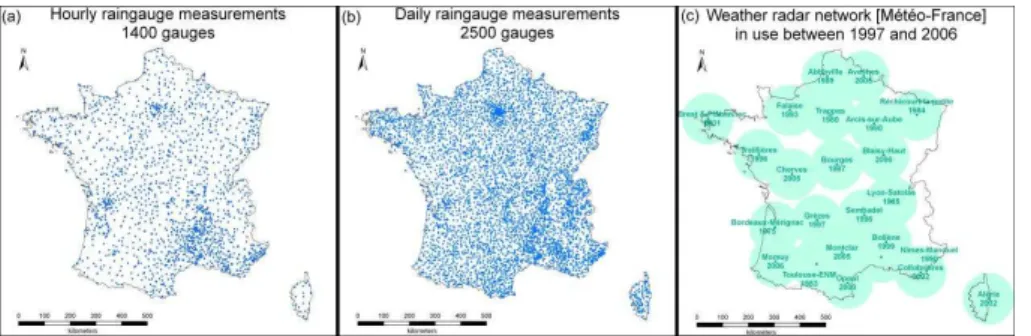
Météo-France, the French national weather service, has recently produced a 10 yr (1997–2006) quantitative precipitation reanalysis at the hourly time step and 1 km2 spatial resolution (Tabary et al., 2012). This reference data set combines all the in-formation available in the operational archives (manual and automatic rain gauges as well as weather radars) in order to obtain the best precipitation estimation over France 15

(550 000 km2). Figure 1 presents the location of available weather radar and rain gauge data in operation between 1997 and 2006. The French operational network was based on 13 radars in 1997 and 10 additional radars have been deployed over the 1997–2006 period, increasing the total number of operational radars to 23 in 2006. The ground measurement network consists of 1400 automatic and 2500 manual rain gauges (from 20

which hourly and daily time series, respectively, can be derived).

We give a short description of the procedure followed by Météo-France to estab-lish the reanalysis, but further detail can be found in Tabary et al. (2012). These data treatments are based on the operational experience of radar data processing at Météo-France. The precipitation data from the rain gauge network are routinely checked and 25

(7)

HESSD

10, 12485–12536, 2013

Title Page

Tables Figures

◭ ◮

Back Close

Full Screen / Esc

Discussion

P

a

per

|

D

iscussion

P

a

per

|

Discussion

P

a

per

|

Discuss

ion

P

a

per

|

dusts, . . . ), partial beam blocking and undersampling eff_{ects before being converted}

into rainfall rates using the Marshall PalmerZ–Rrelationship. Daily calibration factors are computed for every 1 km2pixel by comparing 24 h accumulated radar rainfall rates and daily rain gauge estimates computed from hourly and daily gauge measurements by kriging with external drift. Hourly radar rainfall accumulations are then corrected 5

using the daily calibration factors. Finally, hourly precipitation accumulation fields are computed from the available hourly (calibrated) radar and rain gauge data using kriging with external drift. For the time steps when no radar data are available or in case no calibration factor can be computed, the composite map is filled by ordinary kriging of hourly rain gauge data.

10

The final composite 1 km2hourly rainfall estimates have been successfully validated against independent hourly rain gauge data (not used for the whole reanalysis pro-cess) over 1 yr in southeastern France (Tabary et al., 2012). Hence, the reanalysis can be considered to provide reliable hourly precipitation estimations with high spatial res-olution suitable to investigate the impact of rainfall spatial variability on the catchment 15

response.

2.2 Catchment data set

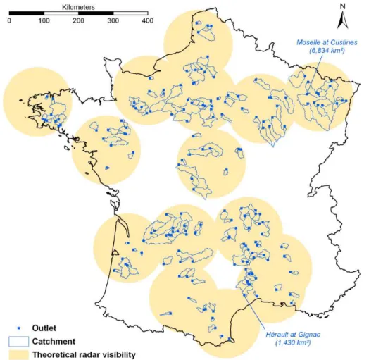
A large set of 181 French catchments (see Fig. 2) was selected to run semi-distributed rainfall-runoff _{simulations. Hourly discharge data at the basin outlets were obtained}

from the HYDRO national archive (www.hydro.eaufrance.fr) for the 10 yr period of the 20

rainfall reanalysis (1997–2006). Since weather radar measurements are considered accurate within a 100 km radius, the catchments were selected within this distance.

The catchment data set represents a wide variety of physiographical and hydrocli-matic conditions (Fig. 2), ranging from oceanic to Mediterranean. This catchment set consists of small to medium-size catchments, with 32 catchments smaller than 100 km2 25

(8)

HESSD

10, 12485–12536, 2013

Title Page

Tables Figures

◭ ◮

Back Close

Full Screen / Esc

Discussion

P

a

per

|

D

iscussion

P

a

per

|

Discussion

P

a

per

|

Discuss

ion

P

a

per

|

range of intensities. Higher values of the rainfall intensity coeffi_{cient (calculated as the}

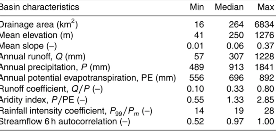
ratio between the 99th percentile and the mean hourly precipitation) and lower values of the streamflow 6 h autocorrelation coeffi_{cient (Table 1) are found in basins located}

in southeastern France in the Cévennes region and Mediterranean area where strong convective storms and flash floods are frequent (Berne et al., 2009; Delrieu et al., 2005; 5

Javelle et al., 2010; Saulnier and Le Lay, 2009). Note that mountainous catchments were intentionally not selected here due to large uncertainties in radar measurements. Hence, there is no significant snow influence in the catchments studied.

3 Methodology

3.1 Semi-distributed rainfall-runoffmodel 10

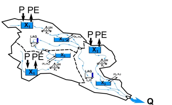
We used a semi-distributed model derived from the work of Lerat (2009). It is based on the GR5H hourly lumped rainfall-runoff_{model proposed by Le Moine (2008) (Fig. 3).}

The GR5H model only has five free parameters (see Fig. 3 and Table 2).

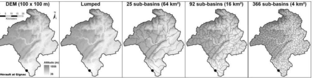
In the semi-distributed model, the catchment is divided into hydrologic units (i.e. sub-catchments) following the drainage network. A digital elevation model was used to build 15

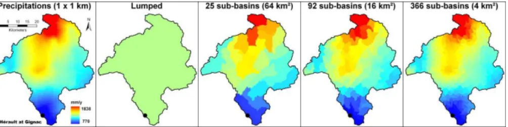
the sub-catchments (O’Callaghan and Mark, 1984). We chose to use sub-catchments of roughly the same size (Fig. 4). Mean rainfall is calculated for each sub-catchment (Fig. 5) and used as input to the GR5H model applied in lumped mode to simulate the outflow of each hydrological unit. Then a channel-routing method is used to route the sub-catchment flows to the downstream catchment outlet through the river network. 20

Given the steep mean slope (greater than 0.01) for all the catchments (Table 1), the kinematic wave approximation can be considered valid to route natural flow in the river network (Henderson, 1966; Morris and Woolhiser, 1980). In this study, the linear lag propagation model (Bentura and Michel, 1997) was found to provide a satisfactory level of effi_{ciency compared to more sophisticated channel routing methods. This is}

(9)

HESSD

10, 12485–12536, 2013

Title Page

Tables Figures

◭ ◮

Back Close

Full Screen / Esc

Discussion

P

a

per

|

D

iscussion

P

a

per

|

Discussion

P

a

per

|

Discuss

ion

P

a

per

|

in agreement with the results of Lerat et al. (2012). This function has a single free parameter: average river flow celerityC (m s−1).

The sensitivity of streamflow simulations to the spatial resolution of rainfall estimates was investigated by testing the semi-distributed rainfall-runoff _{model for three sizes}

of sub-catchments: 64 km2 (SD64), 16 km2 (SD16) and 4 km2 (SD04) (Fig. 4). The 5

number of sub-catchments per catchment ranges between 2 and 108 for SD64, 2 and 432 for SD16, 4 and 1733 for SD04. In each case, the sub-catchment rainfall-runoff

models were fed with rainfall inputs averaged over the sub-catchment, as illustrated in Fig. 5. The lumped configuration was also tested to serve as a reference, using precipitation averaged over the whole catchment as input.

10

3.2 Model parameterization and calibration

The calibration of a distributed or semi-distributed model is a complex task (Carpenter and Georgakakos, 2006; Lerat et al., 2012; Pechlivanidis et al., 2010; Pokhrel and Gupta, 2011) since the number of unknown parameters is magnified, with higher risks of overparameterization, equifinality and non-identifiability issues (Beven, 1993, 1996, 15

2001; Götzinger and Bárdossy, 2007; Kirchner, 2006). Pokhrel and Gupta (2011) even argued that calibration of spatially distributed parameter fields is impossible, since er-rors in model structure and data remain larger than the eff_{ect of spatial variability.}

Here, we deliberately chose to let only the precipitation input vary spatially, while keeping model parameters uniform, in order to focus on the sole impact of spatial vari-20

ability of precipitation on catchment response. This option is supported by the results of previous studies that reported more improvements in model performance related to the spatial distribution of the rainfall input than the distribution of model parameters (Ajami et al., 2004; Andréassian et al., 2004; Boyle et al., 2001). Thus the parameters of the semi-distributed model were constrained to be the same on all sub-catchments. There-25

(10)

HESSD

10, 12485–12536, 2013

Title Page

Tables Figures

◭ ◮

Back Close

Full Screen / Esc

Discussion

P

a

per

|

D

iscussion

P

a

per

|

Discussion

P

a

per

|

Discuss

ion

P

a

per

|

used). Calibration is renewed for each spatial resolution (lumped, SD64, SD16 and SD04) to overcome the scale-sensitivity of model parameters (Bárdossy and Das, 2008; Finnerty et al., 1997; Kumar et al., 2013; Samaniego et al., 2010). Investigat-ing the impact of flow simulation at internal points within the catchment was not within the scope of this study and the reader may refer to Lerat et al. (2012) for a detailed 5

discussion on this issue.

Given the small number of model parameters, the steepest descent local-search pro-cedure used by Editjano et al. (1999) was deemed suffi_{ciently robust to optimize the}

parameters. It was applied with the Kling–Gupta effi_{ciency (KGE) objective function}

(Gupta et al., 2009). The initial parameter set to start optimization is determined by 10

a gross pre-sampling of the parameter space using the discrete sampling method pro-posed by Perrin et al. (2008). This further limits the risk of the procedure being trapped in local optima.

3.3 Method and criteria for the evaluation of streamflow simulations

We performed split-sample calibration-validation tests (Klemeš_{, 1986). The 10 yr study}

15

period (1997–2006) was divided into two independent 5 yr sub-periods (1997–2001 and 2002–2006). Model parameters were calibrated on the first sub-period and model performance was validated on the second one, and vice-versa.

Although the model was continuously run on the periods tested, model performance was evaluated by comparing simulated and observed flow at the outlet of the catchment 20

only for flood events, to focus on the periods when rainfall variability has the greatest influence. For each catchment, the 20 largest floods were selected, leading to a com-plete set of 3620 events (181 catchments×20 events) representing a wide variety of floods. The flood events were automatically selected using the following procedure: (i) the maximum discharge is found, (ii) the beginning (respectively the end) of the event 25

(11)

HESSD

10, 12485–12536, 2013

Title Page

Tables Figures

◭ ◮

Back Close

Full Screen / Esc

Discussion

P

a

per

|

D

iscussion

P

a

per

|

Discussion

P

a

per

|

Discuss

ion

P

a

per

|

the precipitation is null. The threshold dischargeQ₀ is defined for each event, rising limb and declining limb of the hydrograph by Eq. (1):

Q0= max

t_p−240<240<t<t_p t_p<t<t_p+240

Qp/4;Qm+0.05· Qp−Qm

. (1)

where Q_p is the peak flow (i.e., the maximum discharge found), t_p is the time step at which the peak flow is observed,Qm is the minimum discharge observed over the

5

10 day period before (respectively after) the peak flow to calculate the threshold dis-charge needed to define the beginning (respectively the end) of the event.

Table 3 presents the four event-based performance criteria used for the evaluation. KGE (Gupta et al., 2009) measures the overall fit between simulated and observed flows. The peak flow, time to peak and volume errors evaluate the quality of the model 10

simulation on the peak discharge value, timing of the peak discharge and total flow volume of the event, respectively. Note that the peak flow was defined as the maxi-mum discharge, so there was only one peak flow for each event and if several peak flows occurred on the same event only the highest peak flow was considered for the evaluation.

15

The relative performance indexRm[b|a] formulated by Lerat et al. (2012) is used to

compare the performance of modeling optionbto modeling optiona:

Rm[b|a]=

m[Qobs,Qa]−m[Qobs,Qb]

m[Qobs_,Qa_]₊_m[Qobs_,Qb_]. (2)

wheremis a metric measuring the discrepancies between the simulated and observed streamflows which ranges between 0 and infinity (withm=_{0 when the error is null),}_Qa

20

andQb are, respectively, the discharge computed by the model (or the spatial resolu-tion input)aand b. TheRm[b|a] criterion is bounded between−1 and 1 (m=0 when

(12)

HESSD

10, 12485–12536, 2013

Title Page Abstract Introduction Conclusions References Tables Figures ◭ ◮ ◭ ◮ Back Close

Full Screen / Esc

Printer-friendly Version Interactive Discussion Discussion P a per | D iscussion P a per | Discussion P a per | Discuss ion P a per |

3.4 Criteria for the evaluation of rainfall spatial variability

We used two indexes to quantify and compare the spatial variability of precipitation fields: the index of spatial rainfall variability,I_σ, and the location index,IL, proposed by

Smith et al. (2004) and shown in Eqs. (3) and (4) respectively.

Iσ=

T

P

t=1 σt·Pt

T

P

t=1

Pt

, (3)

5

IL=

T

P

t=1

I_pcp(t) .P_t

T

P

t=1

P_t

, (4)

In addition to Eqs. (3) and (4), we also have:

σt =

v u u t

PN

i=1[Pi(t)]

2

N −

h

PN

i=1Pi(t)

i2

N2 , (5)

Ipcp(t)=

C_pcp(t)

Cbsn

, (6)

10

Cpcp(t)=

N

P

i=1

Pi(t)·Ai·Li

N

P

i=1

P_i(t)·A_i

(13)

HESSD

10, 12485–12536, 2013

Title Page

Tables Figures

◭ ◮

Back Close

Full Screen / Esc

Discussion

P

a

per

|

D

iscussion

P

a

per

|

Discussion

P

a

per

|

Discuss

ion

P

a

per

|

Cbsn=

N

P

i=1

A_i·L_i

N

P

i=1

A_i

. (8)

Whereσt is the standard deviation of the hourly precipitation field covering the basin,

P_i(t) is the hourly rainfall data for the pixel i at the time step t,N is the total number of rainfall pixels within the watershed, Cbsn is the basin’s center of mass, Cpcp(t) is

5

the center of rainfall mass for each time step t,Ipcp(t) is the rainfall centroid ratio for

each time step t, Ai is the pixel area (Ai=1 km

2

in the present case) and Li is the

hydraulic distance between the pixeliand the catchment outlet calculated through the river network.

The spatial rainfall variability and location indexes are computed over the hourly 10

gridded (1 km×1 km) rainfall database for each entire flood event. The spatial rain-fall variability index I_σ ranges from 0 to infinity: small values indicate that the spatial variability of the observed rainfall field is low (typical for stratiform events), while high values indicate high spatial variability (convective event). Values of the location index (IL) less than 1 indicate that the largest rainfall amount measured over the event was

15

generally located at the region closest to the outlet, whereas the values greater than 1 indicate that the center of rainfall is far from the outlet.ILvalues close to 1 indicate that

the rainfall and basin centroids coincide.

4 Results and discussion

4.1 Typology of the 3620 observed flood events 20

(14)

HESSD

10, 12485–12536, 2013

Title Page

Tables Figures

◭ ◮

Back Close

Full Screen / Esc

Discussion

P

a

per

|

D

iscussion

P

a

per

|

Discussion

P

a

per

|

Discuss

ion

P

a

per

|

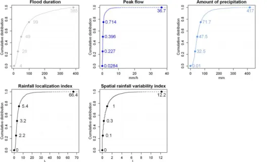
20 events selected for each catchment. About 5 % of events are longer than 490 h (20 days): they are observed in catchments with dominant groundwater contributions, mainly located in northern France (Fig. 7). The mean rainfall amounts at the event scale vary between 1 and 500 mm over the 181 catchments with a mean value equal to 72 mm (Fig. 6). The rainfall amounts greater than 300 mm are observed for 32 5

events with generally short duration (less than 138 h), which are typical of late sum-mer Mediterranean conditions (Fig. 7). The highest peak flow value is observed in the Massane at Argelès-sur-Mer (16 km2, max(Qp)=36.7 mm h

−1

), which is the smallest catchment in the catchment set. Peak flows greater than 4 mm h−1are observed for 111 flood events (3 % of events), which all occurred in the Cévennes and Mediterranean 10

regions: in the Ardèche at Meyras (99 km2, max(Qp)=11.3 mm h−1), the Gardon at

Mialet (244 km2, max(Qp)=10.7 mm h −1

), . . . , and the Hérault at Gignac (1430 km2, max(Q_p)=_{4.3 mm h}−1_).

The median value of the location index is almost equal to 1, which indicates that events are equally distributed between events closer to or farther from the outlet than 15

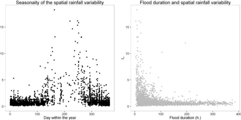
the catchment centroid. The spatial rainfall variability index is quite low (the third quar-tile is less than 1), which means that the precipitation fields in the 3620 observed events are generally stratiform or spatially uniform (Fig. 6). Nevertheless, the spatial rainfall variability index is greater than 1.11 for 20 % of the events, which means that the data set has a significant number of high-variability events (Fig. 6).

20

The localization index is correlated to the spatial rainfall variability index: values far from 1 are usually observed in the regions where high values of the spatial rainfall variability index are also observed (Fig. 7). Indeed, precipitation fields localized close to (or far from) the outlet are most likely to be observed in regions where precipitation fields are spatially variable. In addition, extreme values of the localization index are 25

(15)

HESSD

10, 12485–12536, 2013

Title Page

Tables Figures

◭ ◮

Back Close

Full Screen / Esc

Discussion

P

a

per

|

D

iscussion

P

a

per

|

Discussion

P

a

per

|

Discuss

ion

P

a

per

|

The precipitation fields with a strong spatial variability have short durations (Fig. 8) and they are typically observed between May and October (Fig. 8) in the Mediterranean area (Fig. 7). The largest peak flow coeffi_{cients are also observed in the Mediterranean}

area where the catchments are exposed to summer convective storms with high spatial variability of precipitation fields (Fig. 7). The highest values are obtained in the Ardèche 5

catchment (I_σ=_{4.39) at Vogüé (625 km}2_{), the Hérault catchments and the Gardon}

catchments (I_σ>3.5), which are all located in the Mediterranean area (Fig. 7).

4.2 Impact of spatial rainfall resolution on streamflow simulation efficiency

The impact of spatial rainfall resolution inputs on flow simulation was investigated by comparing model simulations for the four spatial resolutions: (i) lumped, (ii) 64 km2 10

(SD64), (iii) 16 km2(SD16) and (iv) 4 km2(SD04). The results were analyzed by ment classes based on the catchments’ characteristics, shown in Table 1. The catch-ment area and the rainfall intensity coeffi_{cient were found to be the most relevant to}

explain the impact of spatial rainfall resolution on model performance.

Figure 9 presents model performance by catchment classes based on catchment 15

area: the catchment set is divided into three samples of 60 catchments (one sub-sample having 61 catchments). The size ranges from 16 to 155 km2for the G01 group of the smallest catchments and from 497 to 6834 km2for the G03 group of the largest catchments (Fig. 9). Note that for G01, only the smaller sub-catchment size (4 km2) could be tested for all catchments. Therefore, the results for the two other resolutions 20

are not shown.

Some obvious hydrological truths can be observed in Fig. 9:

(i) Model performance is higher for the largest catchments (see, e.g., Merz et al., 2009). Significant diff_{erences were found in model e}ffi_{ciency between the}

smallest-catchment group (G01; ∆_Q_p=_{37 %,} ∆_V=_{26 %,} ∆_t_p=_{0.14, KGE}=_{0.44) and the}

25

largest-catchment group (G04;∆_Q_p=_{21 %,}∆_V=_{16 %,}∆_t_p=_{0.11, KGE}=_0.60).

(16)

HESSD

10, 12485–12536, 2013

Title Page

Tables Figures

◭ ◮

Back Close

Full Screen / Esc

Discussion

P

a

per

|

D

iscussion

P

a

per

|

Discussion

P

a

per

|

Discuss

ion

P

a

per

|

bias (e.g., volume of flow), the relative variability in the simulated and observed values (i.e., the spread of flow) and the coeffi_{cient of correlation (i.e., the timing and shape of}

the hydrograph) (Gupta et al., 2009).

(iii) For all catchment subsets, the lumped model performs almost as well as the semi-distributed model, regardless of the spatial resolution of precipitation input. Only 5

slight improvements were noted with higher spatial resolution in precipitation inputs and they were larger for the largest-catchment sub-sample (group G03). Similar con-clusions were made by Arnaud et al. (2011), for example. In the present study, the KGE averaged over 1200 flood events (for the 60 largest catchments) rose from 0.594 for the lumped model to 0.624 for the semi-distributed model with the finest resolution, and 10

the averaged absolute volume, peak and time to peak errors decreased from 22.4 % to 21.4 %, from 16.4 % to 15.7 % and from 0.112 to 0.108, respectively (Fig. 9).

In Fig. 10, model performance is analyzed by catchment classes based on catch-ment area and the rainfall intensity coeffi_{cient. Each catchment sub-sample (based on}

catchment area) is divided into three sub-classes based on the rainfall intensity coeffi

-15

cient (Table 1). Each sub-class has the same number of catchments (20 catchments) except one having 21 catchments (G01 and low rainfall intensity coeffi_{cient). The low}

rainfall intensity coeffi_{cients range from 17.3 to 19.4 for G01, from 16.8 to 19.0 for G02}

and from 14.3 to 18.0 for G03. The high rainfall intensity coeffi_{cients range from 21.6}

to 27.7 for G01, from 20.9 to 28.3 for G02 and from 19.3 to 25.4 for G03. Note that the 20

rainfall intensity coeffi_{cient (Table 1) was calculated over the whole period of records}

(1997–2006) and was not limited to the selected events (we consider this coeffi_{cient as}

a catchment descriptor).

Model performance was better for catchments with a low rainfall intensity coeffi_cient

for all catchment area groups (Fig. 10). Significant diff_{erences were found in model}

25

effi_{ciency, which decreased when the rainfall intensity coe}ffi_{cient rose: on average,}

between the low and high rainfall intensity coeffi_{cient, the KGE criteria ranged from}

(17)

HESSD

10, 12485–12536, 2013

Title Page

Tables Figures

◭ ◮

Back Close

Full Screen / Esc

Discussion

P

a

per

|

D

iscussion

P

a

per

|

Discussion

P

a

per

|

Discuss

ion

P

a

per

|

The lumped model performed as well as the semi-distributed model regardless of the spatial resolution of precipitation input for catchments with a low rainfall intensity coeffi_{cient. Interestingly, improvements were noted with higher spatial resolution in}

pre-cipitation inputs for catchments with a high rainfall intensity coeffi_{cient (P}

99/Pm>20)

and for all ranges of catchment area (Fig. 10). Although model performance improve-5

ments were slight for the G01 (16–156 km2) and G02 (156–513 km2) catchment groups, significant improvements were obtained for the largest-catchment group (G03: 513– 6834 km2): the KGE averaged over 20 flood events (for the 20 largest catchments with a high rainfall intensity coeffi_{cient) rose from 0.483 for the lumped model to 0.564 for}

the semi-distributed model with the finest resolution. 10

Regardless of the catchment area and rainfall intensity coeffi_{cient, the}

semi-distributed model performed equally well at the diff_{erent spatial resolutions investigated}

(SD64, SD16 and SD04). Indeed, the improvements in streamflow simulation at the catchment outlet between the lumped model and the semi-distributed model at the finest spatial resolution (SD04) were nearly equivalent at coarser spatial resolutions 15

(SD16 and SD64) (Fig. 10).

These results allow generalizing with confidence the conclusions drawn by previous studies (but only obtained over a few catchments) that reported a lack of significant diff_{erences between lumped and semi-distributed flow simulations at the catchment}

outlet (Ajami et al., 2004; Apip et al., 2012; Bell and Moore, 2000; Lindström et al., 20

1997; Naden, 1992; Nicòtina et al., 2008; Obled et al., 1994; Refsgaard and Knud-sen, 1996). However, we found that the impact of higher resolution in precipitation inputs were catchment-dependent since the quality of streamflow simulations was sig-nificantly improved at the outlet of catchments exposed to high rainfall intensity, and these improvements rose with catchment area.

(18)

HESSD

10, 12485–12536, 2013

Title Page

Tables Figures

◭ ◮

Back Close

Full Screen / Esc

Discussion

P

a

per

|

D

iscussion

P

a

per

|

Discussion

P

a

per

|

Discuss

ion

P

a

per

|

4.3 Do criteria describing rainfall spatial variability explain the observed di_fferences?

The previous results were averaged over the 20 flood events for each catchment, which may hide some of the model behavior variability between events, depending on the characteristics of the precipitation fields. This aspect has now been further investi-5

gated. Given the very limited diff_{erences between the three sizes of sub-catchments,}

hereafter we will only consider the lumped and semi-distributed (SD04, finest resolu-tion) simulations. Figure 11 shows the links between the relative performance index (see Eq. 5) applied using the KGE criterion (here notedR_1−KGE) and the indexes of rainfall variability (location index I_L and spatial rainfall variability index I_σ). A positive 10

R_1−KGE criterion indicates that the semi-distributed approach is better than the lumped one, and the reverse is true for negative values.

First of all, it is worth noting that flood events with strong spatial variability of precipi-tation rarely occur compared to stratiform storms with uniform precipiprecipi-tation fields: most of theILvalues are close to 1 andIσ values are generally low (Fig. 11). Interestingly, the

15

medianI_Lvalue rises with catchment area from 0.97 for the smallest-catchment group (G01) to 0.99 for the mid-size catchment group (G02) and up to 1.01 for the largest-catchment group (G03). Similarly, the medianI_σ value rises with catchment area from 0.52 to 0.66 and 0.69 for the G01, G02 and G03 catchment groups, respectively. Thus, the precipitation centroid is generally located at the upstream part of the basin for large 20

catchments and the probability of obtaining uniform spatial rainfall fields is lower in large catchments.

For the small-catchment sub-samples (groups G01 and G02: from 16 to 513 km2), the semi-distributed model (with high spatial resolution of precipitation inputs) and the lumped model (with spatially uniform precipitation inputs) performed equally well 25

(19)

HESSD

10, 12485–12536, 2013

Title Page

Tables Figures

◭ ◮

Back Close

Full Screen / Esc

Discussion

P

a

per

|

D

iscussion

P

a

per

|

Discussion

P

a

per

|

Discuss

ion

P

a

per

|

Nevertheless, for the largest catchments (group G03: from 513 to 6834 km2), the semi-distributed model with high spatial resolution yields better streamflow simulations for the few flood events in which the greatest spatial variability in precipitation fields are observed (high I_σ values or IL<1) (Fig. 11). Interestingly, the semi-distributed model

performed better than the lumped model (for large catchments) for the events where the 5

precipitation fields were located close to the outlet (I_L<1), while the lumped model was able to cope with rainfall fields located far from the outlet (IL>1). This may be due to the

fact that larger precipitation amounts are more often concentrated at the upstream part of the catchment due to an orographic eff_{ect and a strong altitudinal gradient in large}

catchments (Fig. 7). Thus, through calibration the lumped model acquires the ability 10

to accurately reproduce the catchment response for such more common rainfall field patterns, but not for the other “extra-ordinary” (from a precipitation spatial variability point of view) events.

These results – based on a large set of 181 catchments and a wide variety of flood events – clearly show that the impact of spatial variability of precipitation is 15

scale-dependent and event-characteristic-dependent, as suggested by several authors (Ajami et al., 2004; Bell and Moore, 2000; Koren et al., 2004; Segond et al., 2007; Smith et al., 2004; Tetzlaff_{and Uhlenbrook, 2005; Winchell et al., 1998). This may}

ex-plain why contradictory results can be found in the literature on the impacts of spatial rainfall variability on the catchment response: this study shows that some flood events 20

are improved using higher spatial rainfall information and others are not (Fig. 11).

4.4 Which catchments should be modeled in a semi-distributed way?

Here we investigate the possibility of identifying catchments where a spatially dis-tributed representation would bring a definite advantage. Figure 12 shows the com-parison between lumped and semi-distributed simulations evaluated by the relative 25

(20)

HESSD

10, 12485–12536, 2013

Title Page

Tables Figures

◭ ◮

Back Close

Full Screen / Esc

Discussion

P

a

per

|

D

iscussion

P

a

per

|

Discussion

P

a

per

|

Discuss

ion

P

a

per

|

events each). The analysis based on the 3620 observed flood events shows that the re-sults are contrasted (Fig. 12): 44 % of flood events are better simulated with the lumped model (fed with spatially uniform precipitation inputs). Using higher spatial resolution of precipitation inputs only improves model performance for a small majority (56 %). It is diffi_{cult to draw conclusions given the low median value of the relative performance}

5

index, equal to 0.006 (Fig. 12).

However, when the large set of flood events is analyzed by catchment (Fig. 12, right), these contrasted results appear to be catchment-dependent: spatial precipitation inputs greatly improve the streamflow simulations at the outlets of some catchments, whereas the impact of spatial forcing is insignificant or semi-distributed modeling is worse than 10

lumped modeling for other catchments (Fig. 12). These findings highlight the need to test model hypotheses on large and diversified catchment sets (Andréassian et al., 2009).

4.5 Can specific catchment behaviors be explained?

To identify the catchments that benefit (or not) from higher-resolution rainfall informa-15

tion, the relative performance indexes calculated over 20 flood events (Fig. 12) were averaged by catchment. The cumulative distribution of the mean relative performance index and the geographic localization for the 181 catchments are shown in Fig. 13. The performance of the lumped model was better than the semi-distributed model for 39 % of catchments. Hence the semi-distributed approach appears beneficial for 61 % of the 20

catchment set (Fig. 13).

The analysis applied independently for each catchment pointed out regional ten-dencies concerning the impact of spatial rainfall resolution on streamflow simulation (Fig. 13). In western France, streamflow simulation at the outlets of the catchments located close to the Atlantic coast were not improved when using higher spatial rainfall 25

(21)

HESSD

10, 12485–12536, 2013

Title Page

Tables Figures

◭ ◮

Back Close

Full Screen / Esc

Discussion

P

a

per

|

D

iscussion

P

a

per

|

Discussion

P

a

per

|

Discuss

ion

P

a

per

|

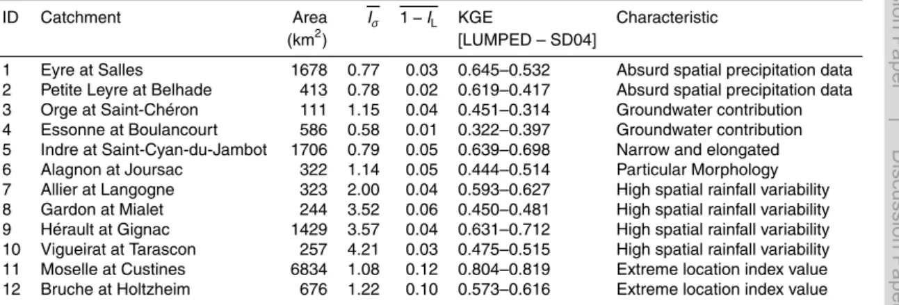
catchments, the Petite Leyre and the Eyre catchments (Fig. 13 and Table 5), exhibited strong model performance decreases when used in spatial distribution mode. Detailed analysis showed that the semi-distributed model was aff_{ected by absurdly high values}

in spatial precipitation data inputs coming from radar measurements (despite the treat-ments applied to correct them and the numerous quality checks). These inaccurate 5

precipitation values were smoothed by averaging the spatial precipitation data over the catchment in the lumped model. As a result, the lumped model successfully computed the flow at the catchment’s outlets, contrary to the semi-distributed model.

In northern France, the results were contrasted. In this region, many catchments are influenced by significant groundwater contribution. Model performance remained low 10

on these catchments whatever the spatial distribution (Fig. 13): for example, for the Es-sonne catchment, the KGE value increased from 0.322 with the lumped model to only 0.397 with the semi-distributed model (Table 5). Increasing spatial information in precip-itation inputs did not necessarily yield better flow simulations and strong decreases in model performance could be observed between the lumped and the semi-distributed 15

model (Fig. 13 and Table 5). Our interpretation is that (i) spatial rainfall variability is already quite low in this region (Fig. 7), while (ii) the impact of spatially variable precip-itation is dampened by the high infiltrability in this catchment dominated by subsurface flow (Nicòtina et al., 2008).

The catchments that benefit most from higher spatial resolution of precipitation inputs 20

(Fig. 13) are the catchments in which precipitation fields are identified to be significantly variable in space (Fig. 7). We identified two regions strongly exposed to spatial rainfall variability: the Cévennes and Mediterranean regions in southern France with high spa-tial rainfall indexes (Fig. 7) and northeastern France with extreme location index values (Fig. 7). As examples, we present three flood events with high spatial rainfall variability 25

that occurred on the large Hérault catchment (1430 km2) and the medium-size Allier (323 km2) and Alagnon catchments (322 km2). The observed precipitation fields were highly variable in space, as indicated by the high values of the spatial rainfall vari-ability index: I_σ=_{6.73 (September 2000),} _I

(22)

HESSD

10, 12485–12536, 2013

Title Page

Tables Figures

◭ ◮

Back Close

Full Screen / Esc

Discussion

P

a

per

|

D

iscussion

P

a

per

|

Discussion

P

a

per

|

Discuss

ion

P

a

per

|

(October 2003). As a consequence, the simulated peak flow was well depicted with the semi-distributed model due to spatially distributed precipitation inputs, whereas it was missed with spatially uniform precipitation input in lumped modeling (Fig. 14). Similar conclusions were reached for two catchments in northeastern France and one Cévennes catchment where extreme location index values were identified: the quality 5

of streamflow simulations was improved due to higher spatial rainfall information within the semi-distributed model (Fig. 15).

5 Conclusions

5.1 Summary

The impact of higher-resolution rainfall information on streamflow simulation was in-10

vestigated over a large set of 3620 flood events selected on 181 French catchments. Semi-distributed streamflow simulations were run at diff_{erent spatial resolutions and}

evaluated against observed flow data at catchment outlets. The results were analyzed (i) by catchment classes based on catchment area and (ii) by flood events based on the spatial variability of observed precipitation fields.

15

This study first confirms that on average, the diff_{erences in model performance}

be-tween lumped and semi-distributed options are not significant. However, the analysis applied by catchment and by flood event clearly showed that the impact of spatial rain-fall information on flow simulation is scale-dependent, catchment-dependent and event characteristic-dependent. This result underlines that catchment response to spatial het-20

erogeneity of precipitation fields is highly variable between catchments.

The catchments’ size and the rainfall intensity coeffi_{cient were shown to be e}ff_ective

(23)

HESSD

10, 12485–12536, 2013

Title Page

Tables Figures

◭ ◮

Back Close

Full Screen / Esc

Discussion

P

a

per

|

D

iscussion

P

a

per

|

Discussion

P

a

per

|

Discuss

ion

P

a

per

|

simulation were obtained at the outlet of large catchments and for events with signifi-cant spatial variability in precipitation fields.

By investigating catchment responses independently for each catchment and for a variety of flood events, regional tendencies were pointed out concerning the po-tential benefit of high spatial rainfall resolution for runoff _{modeling in France. While}

5

a better spatial representation of precipitation inputs did not yield better streamflow simulations at the outlet of catchments exposed to oceanic climate conditions, signif-icant improvements were obtained in regions frequently exposed to rainstorms with high spatial variability, such as the Cévennes and the Mediterranean regions.

These results highlight the need to work on large and varied sets of catchments 10

(Gupta et al., 2013). Catchment dependency on rainfall spatial variability is confirmed. By carefully analyzing the changes in simulated hydrographs at diff_{erent spatial}

reso-lutions, the significant influence on particular sub-catchments can be detected. In this way, the methodology applied in this study provides insights to investigate the catch-ment properties that may influence the catchcatch-ment response.

15

5.2 Limits and perspectives

In spite of our eff_{ort to obtain general results, we do see some limits to our conclusions.}

First of all, we must mention that the results may still be somewhat dependent on the model or testing methodology used, which may not be adapted to certain particular basin behaviors (Pokhrel et al., 2012; Smith et al., 2012). Here, we have applied a sin-20

gle model structure to all catchments, where others would have preferred catchment-specific structures (Fenicia et al., 2011). The spatial heterogeneities in catchment char-acteristics may interact with the spatial heterogeneity in precipitation fields, with the risk of masking the impact of spatial rainfall variability. Working on optimizing the model structure on a catchment-by-catchment basis could help resolve a few surprising re-25

(24)

HESSD

10, 12485–12536, 2013

Title Page

Tables Figures

◭ ◮

Back Close

Full Screen / Esc

Discussion

P

a

per

|

D

iscussion

P

a

per

|

Discussion

P

a

per

|

Discuss

ion

P

a

per

|

a few catchments in central France (Fig. 13 and Table 5), although these catchments were not exposed to strong spatial rainfall variability (Fig. 7), but they are long catch-ments with a particular morphology where streamflow simulations may benefit from the channel-routing function of the semi-distributed model. These particular catchments need complementary analysis to validate these hypotheses, which is beyond the scope 5

of this paper.

At this point, we see a natural continuation of this work in further investigations with models whose parameters will be allowed to be distributed spatially, in order to explore the impact of catchment heterogeneities on catchment response. In our opinion, how-ever, this complementary work should not fundamentally modify the conclusions of this 10

paper.

Acknowledgements. The authors thank Météo-France and SCHAPI for providing meteorologi-cal and hydrologimeteorologi-cal data, respectively.

References

Ajami, N. K., Gupta, H. V., Wagener, T., and Sorooshian, S.: Calibration of a semi-distributed 15

hydrologic model for streamflow estimation along a river system, J. Hydrol., 298, 112–135, doi:10.1016/j.jhydrol.2004.03.033, 2004.

Andréassian, V., Perrin, C., Michel, C., Usartsanchez, I., and Lavabre, J.: Impact of imperfect rainfall knowledge on the efficiency and the parameters of watershed models, J. Hydrol., 250, 206–223, doi:10.1016/S0022-1694(01)00437-1, 2001.

20

Andréassian, V., Oddos, A., Michel, C., Anctil, F., Perrin, C., and Loumagne, C.: Impact of spatial aggregation of inputs and parameters on the effi_{ciency of rainfall-runo}ff_{models: a theoretical} study using chimera watersheds, Water Resour. Res., 40, 1–9, doi:10.1029/2003WR002854, 2004.

Andréassian, V., Perrin, C., Berthet, L., Le Moine, N., Lerat, J., Loumagne, C., Oudin, L., Math-25

(25)

HESSD

10, 12485–12536, 2013

Title Page

Tables Figures

◭ ◮

Back Close

Full Screen / Esc

Discussion

P

a

per

|

D

iscussion

P

a

per

|

Discussion

P

a

per

|

Discuss

ion

P

a

per

|

Apip, Sayama, T., Tachikawa, Y., and Takara, K.: Spatial lumping of a distributed rainfall-sediment-runoff _{model and its e}ff_{ective lumping scale, Hydrol. Process., 26, 855–871,} doi:10.1002/hyp.8300, 2012.

Arnaud, P., Bouvier, C., Cisneros, L., and Dominguez, R.: Influence of rainfall spatial variability on flood prediction, J. Hydrol., 260, 216–230, doi:10.1016/S0022-1694(01)00611-4, 2002. 5

Arnaud, P., Lavabre, J., Fouchier, C., Diss, S., and Javelle, P.: Sensitivity of hy-drological models to uncertainty in rainfall input, Hydrolog. Sci. J., 56, 397–410, doi:10.1080/02626667.2011.563742, 2011.

Bárdossy, A. and Das, T.: Influence of rainfall observation network on model calibration and application, Hydrol. Earth Syst. Sci., 12, 77–89, doi:10.5194/hess-12-77-2008, 2008. 10

Bell, V. A. and Moore, R. J.: The sensitivity of catchment runoff_{models to rainfall data at di}ff_erent spatial scales, Hydrol. Earth Syst. Sci., 4, 653–667, doi:10.5194/hess-4-653-2000, 2000. Bentura, P. and Michel, C.: Flood routing in a wide channel with a quadratic lag-and-route

method, Hydrolog. Sci. J., 42, 169–189, doi:10.1080/02626669709492018, 1997.

Berne, A., Delrieu, G., Creutin, J. D., and Obled, C.: Temporal and spatial resolu-15

tion of rainfall measurements required for urban hydrology, J. Hydrol., 299, 166–179, doi:10.1016/j.jhydrol.2004.08.002, 2004.

Berne, A., Delrieu, G., and Boudevillain, B.: Variability of the spatial structure

of intense Mediterranean precipitation, Adv. Water Resour., 32, 1031–1042,

doi:10.1016/j.advwatres.2008.11.008, 2009. 20

Beven, K.: Prophecy, reality and uncertainty in distributed hydrological modelling, Adv. Water Resour., 16, 41–51, doi:10.1016/0309-1708(93)90028-E, 1993.

Beven, K.: The limits of splitting: hydrology, Sci. Total. Environ., 183, 89–97, doi:10.1016/0048-9697(95)04964-9, 1996.

Beven, K.: How far can we go in distributed hydrological modelling?, Hydrol. Earth Syst. Sci., 25

5, 1–12, doi:10.5194/hess-5-1-2001, 2001.

Beven, K. and Hornberger, G. M.: Assessing the eff_{ect of spatial pattern of precipitation in} mod-eling streamflow hydrographs, J. Am. Water Resour. As., 18, 823–829, doi:10.1111/j.1752-1688.1982.tb00078.x, 1982.

Bonnifait, L., Delrieu, G., Le Lay, M., Boudevillain, B., Masson, A., Belleudy, P., Gaume, E., and 30

(26)

HESSD

10, 12485–12536, 2013

Title Page

Tables Figures

◭ ◮

Back Close

Full Screen / Esc

Discussion

P

a

per

|

D

iscussion

P

a

per

|

Discussion

P

a

per

|

Discuss

ion

P

a

per

|

Boyle, D. P., Gupta, H. V., Koren, V., Zhang, Z., and Smith, M. B.: Toward improved streamflow forecasts: Value of semidistributed modeling, Water Resour., 37, 2749–2759, 2001.

Carpenter, T. and Georgakakos, K. P.: Intercomparison of lumped versus distributed hydro-logic model ensemble simulations on operational forecast scales, J. Hydrol., 329, 174–185, doi:10.1016/j.jhydrol.2006.02.013, 2006.

5

Carpenter, T., Georgakakos, K. P., and Sperfslagea, J.: On the parametric and NEXRAD-radar sensitivities of a distributed hydrologic model suitable for operational use, J. Hydrol., 253, 169–193, doi:10.1016/S0022-1694(01)00476-0, 2001.

Cole, S. J. and Moore, R. J.: Hydrological modelling using raingauge- and radar-based estima-tors of areal rainfall, J. Hydrol., 358, 159–181, doi:10.1016/j.jhydrol.2008.05.025, 2008. 10

Das, T., Bárdossy, A., Zehe, E., and He, Y.: Comparison of conceptual model perfor-mance using diff_{erent representations of spatial variability, J. Hydrol., 356, 106–118,} doi:10.1016/j.jhydrol.2008.04.008, 2008.

Delrieu, G., Nicol, J., Yates, E., Kirstetter, P.-E., Creutin, J.-D., Anquetin, S., Obled, C., Saulnier, G.-M., Ducrocq, V., Gaume, E., Payrastre, O., Andrieu, H., Ayral, P.-A., Bouvier, C., 15

Neppel, L., Livet, M., Lang, M., Du-Châtelet, J. P., Walpersdorf, A., and Wobrock, W.: The catastrophic flash-flood event of 8–9 September 2002 in the Gard Region, France: a first case study for the Cévennes–Vivarais Mediterranean Hydrometeorological Observatory, J. Hydrometeorol., 6, 34–52, doi:10.1175/JHM-400.1, 2005.

Dodov, B. and Foufoula-Georgiou, E.: Incorporating the spatio-temporal distribution of rainfall 20

and basin geomorphology into nonlinear analyses of streamflow dynamics, Adv. Water Re-sour., 28, 711–728, doi:10.1016/j.advwatres.2004.12.013, 2005.

Editjano, Nascimento, N., Yang, X., Makhlouf, Z., and Michel, C.: GR3J: a daily

watershed model with three free parameters, Hydrol. Sci. J., 44, 263–277,

doi:10.1080/02626669909492221, 1999. 25

Emmanuel, I., Andrieu, H., Leblois, E., and Flahaut, B.: Temporal and spatial vari-ability of rainfall at the urban hydrological scale, J. Hydrol., 430–431, 162–172, doi:10.1016/j.jhydrol.2012.02.013, 2012.

Faures, J., Goodrich, D. C., Woolhiser, D. A., and Sorooshian, S.: Impact of small-scale spatial rainfall variability on runoff _{modeling, J. Hydrol., 173, 309–326,} doi:10.1016/0022-30

(27)

HESSD

10, 12485–12536, 2013

Title Page

Tables Figures

◭ ◮

Back Close

Full Screen / Esc

Discussion

P

a

per

|

D

iscussion

P

a

per

|

Discussion

P

a

per

|

Discuss

ion

P

a

per

|

Fenicia, F., Kavetski, D., and Savenije, H. H. G.: Elements of a flexible approach for conceptual hydrological modeling: 1. Motivation and theoretical development, Water Resour. Res., 47, 1–13, doi:10.1029/2010WR010174, 2011.

Finnerty, B., Smith, M. B., Seo, D., Koren, V., and Moglen, G.: Space-time scale sensitiv-ity of the Sacramento model to radar-gage precipitation inputs, J. Hydrol., 203, 21–38, 5

doi:10.1016/S0022-1694(97)00083-8, 1997.

Götzinger, J. and Bárdossy, A.: Comparison of four regionalisation methods for a distributed hydrological model, J. Hydrol., 333, 374–384, doi:10.1016/j.jhydrol.2006.09.008, 2007. Gupta, H. V., Kling, H., Yilmaz, K. K., and Martinez, G. F.: Decomposition of the mean squared

error and NSE performance criteria: Implications for improving hydrological modelling, J. 10

Hydrol., 377, 80–91, doi:10.1016/j.jhydrol.2009.08.003, 2009.

Gupta, H. V., Perrin, C., Kumar, R., Blöschl, G., Clark, M., Montanari, A., and Andréassian, V.: Large-sample hydrology: a need to balance depth with breadth, Hydrol. Earth Syst. Sci. Discuss., 10, 9147–9189, doi:10.5194/hessd-10-9147-2013, 2013.

Henderson, F. M.: Open Channel Flow, Macmillan, Prentice Hall, New York, 1966. 15

Javelle, P., Fouchier, C., Arnaud, P., and Lavabre, J.: Flash flood warning at ungauged loca-tions using radar rainfall and antecedent soil moisture estimaloca-tions, J. Hydrol., 394, 267–274, doi:10.1016/j.jhydrol.2010.03.032, 2010.

Kampf, S. K. and Burges, S. J.: A framework for classifying and comparing dis-tributed hillslope and catchment hydrologic models, Water Resour. Res., 43, W05423, 20

doi:10.1029/2006WR005370, 2007.

Kirchner, J. W.: Getting the right answers for the right reasons: linking measurements, anal-yses, and models to advance the science of hydrology, Water Resour. Res., 42, W03S04, doi:10.1029/2005WR004362, 2006.

Klemeš_{, V.: Operational testing of hydrological simulation models/Vérification, en} condi-25

tions réelles, des modèles de simulation hydrologique, Hydrolog. Sci. J., 31, 13–24, doi:10.1080/02626668609491024, 1986.

Koren, V., Finnerty, B., Schaake, J., Smith, M. B., Seo, D., and Duan, Q.: Scale dependen-cies of hydrologic models to spatial variability of precipitation, J. Hydrol., 217, 285–302, doi:10.1016/S0022-1694(98)00231-5, 1999.

30