Assessment of high-resolution satellite rainfall for streamflow simulation in medium watersheds of the East African highlands

(1)

HESSD

7, 8213–8232, 2010

High-resolution satellite rainfall

M. M. Bitew and M. Gebremichael

Title Page

Abstract Introduction

Conclusions References

Tables Figures

◭ ◮

Back Close

Full Screen / Esc

Printer-friendly Version Interactive Discussion

Discussion

P

a

per

|

Dis

cussion

P

a

per

|

Discussion

P

a

per

|

Discussio

n

P

a

per

|

Hydrol. Earth Syst. Sci. Discuss., 7, 8213–8232, 2010 www.hydrol-earth-syst-sci-discuss.net/7/8213/2010/ doi:10.5194/hessd-7-8213-2010

Hydrology and Earth System Sciences Discussions

This discussion paper is/has been under review for the journal Hydrology and Earth System Sciences (HESS). Please refer to the corresponding final paper in HESS if available.

Assessment of high-resolution satellite

rainfall for streamflow simulation in

medium watersheds of the East African

highlands

M. M. Bitew and M. Gebremichael

Department of Civil and Environmental Engineering, University of Connecticut, Connecticut, USA

Received: 26 July 2010 – Accepted: 3 August 2010 – Published: 18 October 2010

Correspondence to: M. Gebremichael (mekonnen@engr.uconn.edu)

(2)

HESSD

7, 8213–8232, 2010

Title Page

Tables Figures

◭ ◮

Back Close

Full Screen / Esc

Discussion

P

a

per

|

Dis

cussion

P

a

per

|

Discussion

P

a

per

|

Discussio

n

P

a

per

|

Abstract

The objective is to assess the suitability of commonly used high-resolution satellite rainfall products (CMORPH, TMPA 3B42RT, TMPA 3B42 and PERSIANN) as input to the semi-distributed hydrological model SWAT for daily streamflow simulation in two watersheds (Koga at 299 km2 and Gilgel Abay at 1656 km2) of the East African

high-5

lands. First, the model is calibrated for each watershed with respect to each rainfall product input for the period 2003–2004. Then daily streamflow simulations for the val-idation period 2006–2007 are made from SWAT using rainfall input from each source and corresponding model parameters; comparison of the simulations to the observed streamflow at the outlet of each watershed forms the basis for the conclusions of this

10

study. Results reveal that the utility of satellite rainfall products as input to SWAT for daily streamflow simulation strongly depends on the product type. The 3B42RT and CMORPH simulations show consistent and modest skills in their simulations but un-derestimate the large flood peaks, while the 3B42 and PERSIANN simulations have in-consistent performance with poor or no skills. Not only are the microwave-based

algo-15

rithms (3B42RT, CMORPH) better than the infrared-based algorithm (PERSIANN), but the infrared-based algorithm PERSIANN also has poor or no skills for streamflow sim-ulations. The only product (3B42RT) performs much better than the satellite-gauge product (3B42), indicating that the algorithm used to incorporate rain satellite-gauge information with the goal of improving the accuracy of the satellite rainfall products is

20

actually making the products worse, pointing to problems in the algorithm. The effect of watershed area on the suitability of satellite rainfall products for streamflow simula-tion also depends on the rainfall product. Increasing the watershed area from 299 km2 to 1656 km2 improves the simulations obtained from the 3B42RT and CMORPH (i.e. products that are more reliable and consistent) rainfall inputs while it deteriorates the

25

(3)

HESSD

7, 8213–8232, 2010

Title Page

Tables Figures

◭ ◮

Back Close

Full Screen / Esc

Discussion

P

a

per

|

Dis

cussion

P

a

per

|

Discussion

P

a

per

|

Discussio

n

P

a

per

|

1 Introduction

Prediction of streamflow simulation in ungauged basins of the East African highlands is a challenging task due to the absence of reliable ground-based rainfall information. The region has no any weather radar, the rain gauge distribution is very sparse, and coun-tries in the downstream of transboundary river basins have no access to the existing

5

upstream rain gauge information. Can high-resolution satellite-based rainfall estimates provide reliable rainfall information for streamflow simulation application in this region? During the last two decades, satellite-based instruments have been designed to col-lect observations mainly at thermal infrared (IR) and microwave (MW) wavelengths that can be used to estimate rainfall rates. Observations in the IR band are available

10

in passive modes from (near) polar-orbiting (revisit times of 1–2 days) and geostation-ary orbits (revisit times of 15–30 min), while observations in the passive and active MW band are only available from the (near) polar-orbiting satellites. A number of al-gorithms have been developed to estimate rainfall rates by combining information from the more accurate (but infrequent) MW with the more frequent (but less accurate) IR

15

to take advantage of the complementary strengths. The TMPA method (Huffman et al., 2007) uses MW data to calibrate the IR-derived estimates and creates estimates that contain MW-derived rainfall estimates when and where MW data are available and the calibrated IR estimates where MW data are not available. The TMPA products are available in two versions: real-time version (3B42RT) and post-real-time research

20

version (3B42). The main difference between the two versions is the use of monthly rain gauge data for bias adjustment in the post-real-time research product. The 3B42 products are released 10–15 days after the end of each month, while the 3B42RT are released about 9 h after overpass. The CMORPH method (Joyce et al., 2004) ob-tains the rainfall estimates from MW data but uses a tracking approach in which IR

25

(4)

HESSD

7, 8213–8232, 2010

Title Page

Tables Figures

◭ ◮

Back Close

Full Screen / Esc

Discussion

P

a

per

|

Dis

cussion

P

a

per

|

Discussion

P

a

per

|

Discussio

n

P

a

per

|

to the IR data to generate rainfall estimates. The resolutions of these (often dubbed as “high-resolution”) products are 0.25◦ _{and 3 hourly, although finer resolutions are}

also available for CMORPH and PERSIANN. Besides these widely known products, there are also other high-resolution products, such as, Hydro-estimator (Scofield and Kuligowski, 2003), NRL-blended (Turk and Miller, 2005), PMIR (Kidd and Muller, 2009),

5

and GSMaP (Ushio and Kachi, 2009).

It is well known that the satellite rainfall values are just estimates that are subject to errors arising from the observations, revisiting times and algorithms. However, there is no quantitative information on the estimation errors associated with the operational satellite rainfall products. Consequently, hydrologists of the East African highlands do

10

not know the capability and limitation of the satellite rainfall products for streamflow simulation, and which products to select.

The purpose of this study is to assess the capability and limitation of satellite rainfall products as input into a hydrological model for streamflow simulation in the East African highlands. This study is limited to the following specific cases: the Soil and Water

As-15

sessment Tool (SWAT) hydrological model, two watersheds (299 km2, and 1656 km2), and four satellite precipitation products (TMPA 3B42, TMPA 3B42RT, CMORPH, and PERSIANN). SWAT is a semi-distributed hydrological model widely used for research and application, and according to Gassman et al. (2007) over 250 peer-reviewed jour-nal articles existed by 2007 on SWAT-related work.

20

2 Data and method 2.1 Study region

The study region consists of two gauged adjoining watersheds (Koga and Gilgel Abay) in the Ethiopian part of the East African highlands (Fig. 1). Koga watershed has a drainage area of 299 km2and is located within 37◦₂′_E–37◦₂₀′_{E and 11}◦₈′_N–11◦₂₅′_N, 25

(5)

HESSD

7, 8213–8232, 2010

Title Page

Tables Figures

◭ ◮

Back Close

Full Screen / Esc

Discussion

P

a

per

|

Dis

cussion

P

a

per

|

Discussion

P

a

per

|

Discussio

n

P

a

per

|

37◦₂₄′_{E and 10}◦₅₆′_N–11◦₂₃′_{N. The climate is semi-humid with a mean annual rainfall}

of 1300 mm, more than 70% of which falls in the summer monsoon season. The wa-tersheds have similar landscape characteristics: complex topography with elevations ranging from 1890 m to 3130 m (for Koga), and 1880 m to 3530 m (for Gilgel Abay); land use characterized by cropland, pasture and forest shrubs (55%, 20%, and 25%,

5

respectively for Koga, and 74%, 15%, and 11%, respectively, for Gilgel Abay), and soils characterized by clay, clay loam and silt loam (42%, 39%, and 19%, respectively for Koga, and 33%, 34%, and 33%, respectively, for Gilgel Abay). There are four rain gauges in the study region, and stream gauge at the outlet of each watershed.

2.2 Hydrological model and calibration

10

2.2.1 SWAT hydrological model

SWAT, developed by the United States Department of Agriculture (USDA) – Agricultural Research Service (ARS) (Arnold et al., 1998), is a continuous, semi-distributed hydro-logic model that runs on a daily time step. Hydrohydro-logic response units (HRUs), defined by combinations of land cover and soil combinations, are the computational elements

15

of SWAT. The daily water budget in each HRU is computed based on daily precipita-tion, runo_ff, evapotranspiration, percolation, and return flow from the subsurface and groundwater flow. Runoffvolume in each HRU is computed using the Soil Conserva-tion Service (SCS) curve number method (SCS, 1986). A complete descripConserva-tion of the SWAT model can be found in Arnold et al. (1998). We obtained the following SWAT

20

inputs: elevation data from the 30-m USGS NED digital elevation model dataset, soil texture from the FAO East Africa dataset, land use from the Ethiopian Woody Biomass Inventory Strategic Planning Project, meteorological data from the nearby meteorolog-ical station, and rainfall data from satellite rainfall estimates and rain gauge measure-ments.

(6)

HESSD

7, 8213–8232, 2010

Title Page

Tables Figures

◭ ◮

Back Close

Full Screen / Esc

Discussion

P

a

per

|

Dis

cussion

P

a

per

|

Discussion

P

a

per

|

Discussio

n

P

a

per

|

2.2.2 Parameter specification and calibration

Automatic calibration of all the SWAT model parameters could be time consuming and less practical (Eckhardt and Arnold, 2001). In order to reduce the number of calibra-tion parameters, we performed sensitivity analysis using the LH-OAT method available within SWAT, which combines the Latin Hypercube (LH) sampling method with the

5

One-factor-At-a-Time (OAT) method (Van Griensven et al., 2006). We found nine most sensitive parameters, and focused our automatic and manual calibration exercise on these parameters. Our objective function was maximizing the Nash-Sutcliffe efficiency between simulated and measured daily streamflow.

We calibrated the model parameters for each watershed and rainfall input source,

10

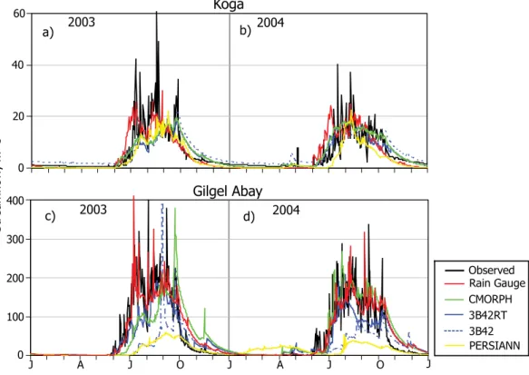
separately, over a two-year period (2003–2004) by comparing the simulated and ob-served daily streamflow hydrographs. The resulting model parameter estimates are shown in Table 1. Comparison between simulated and observed streamflow hydro-graphs is shown in Fig. 2. In general, the simulation results are satisfactory for Koga. For Gilgel Abay, the calibration results for the 3B42RT, CMORPH and rain gauge

sim-15

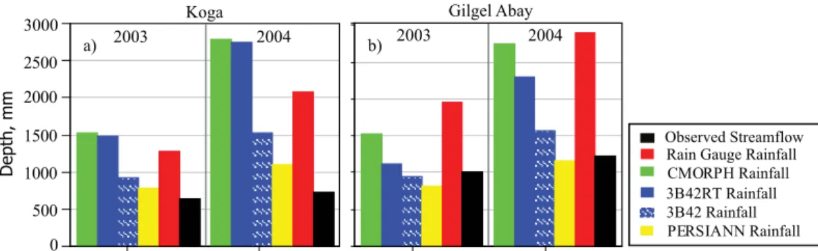
ulations show satisfactory calibration results, whereas the results for 3B42 and PER-SIANN are not satisfactory. As can be seen from Fig. 3b, the 3B42 and PERPER-SIANN products give annual rainfall estimates that are lower than the annual streamflow esti-mates, while the other rainfall products give rainfall estimates substantially higher than the streamflow depth. This indicates that the lack of satisfactory calibration results for

20

3B42 and PERSIANN over Gilgel Abay is reflective of the substantial underestimation bias in the 3B42 and PERSIANN rainfall estimates.

2.3 Approach and performance statistics

We used rainfall data from each source (3B42RT, 3B42, CMORPH, PERSIANN, and rain gauges) for the validation period 2006 to 2007 as input into SWAT with model

25

(7)

HESSD

7, 8213–8232, 2010

M. M. Bitew and M. Gebremichael Title Page Abstract Introduction Conclusions References Tables Figures ◭ ◮ ◭ ◮ Back Close

Full Screen / Esc

Printer-friendly Version Interactive Discussion Discussion P a per | Dis cussion P a per | Discussion P a per | Discussio n P a per |

CMORPH rainfall input) and watershed to simulate daily streamflow. We assess the performance accuracy of each simulation by comparison with observed streamflow. The comparison is made based on visual inspection of hydrographs and exceedance probabilities, and through the following performance statistics: coefficient of determi-nation (R2), relative bias (Rbias), and Nash-Sutcliffe efficiency (NSE):

5

R2 ₌

       n P i₌1

SIMi − SIM¯

OBSi − OBS¯

s n P i₌1

SIMi − SIM¯ 2

s n P i₌1

OBSi − OBS¯ 2        2 Rbias = n P i₌1

(SIMi − OBSi)

n P i₌1

OBSi

NSE ₌ 1 ₋

     n P i₌1

(SIMi − OBSi) 2

n P i=1

OBSi − OBS¯ 2      ,

where SIM is the simulated daily streamflow, OBS is the observed daily streamflow, nis the total number of pairs of simulated and observed data, and the bar indicates

10

average value over n. NSE indicates how well the plot of the observed value versus the simulated value fits the 1:1 line, and ranges from −∞ to 1, with higher values

indicating better agreement (Legates and McCabe, 1999). R2 measures the variance of observed values explained by the simulated values. Rbias measures the relative error in total streamflow volume.

(8)

HESSD

7, 8213–8232, 2010

Title Page

Tables Figures

◭ ◮

Back Close

Full Screen / Esc

Discussion

P

a

per

|

Dis

cussion

P

a

per

|

Discussion

P

a

per

|

Discussio

n

P

a

per

|

3 Results and discussion

We simulated daily streamflow for the validation period 2006–2007 from SWAT using rainfall input from each source and corresponding model parameters. In this section, we discuss the accuracy of the simulations.

3.1 Koga watershed

5

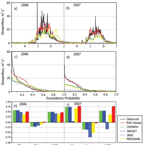
Comparisons of simulated and observed streamflow for Koga watershed are given in Fig. 4. Let us first discuss the results for 2006. According to Fig. 4a, all simulations capture the overall shape of observed streamflow hydrographs, but underestimate the large flood peaks, with the rain gauge simulations showing better performance than the satellite simulations. The 3B42RT and CMORPH simulations are identical. Figure 4c

10

shows that all simulations underestimate the frequency of the extreme events with probabilities of exceedance lower than 5%; the underestimations are severe for satel-lite rainfall simulations compared to the rain gauge simulations. According to Fig. 4e, theR2 values for the time series of daily streamflow between simulated and observed values vary in the range 0.4 to 0.6; the satellite rainfall simulations underestimate the

15

total streamflow volume by 10% to 20%, while the rain gauge simulations give almost accurate results; the NSE values, ranging from 0.4 to 0.5, indicate that all the simula-tions exhibit moderate skills in reproducing daily streamflow.

Do the performance accuracy results hold in 2007? According to Fig. 4b, the 3B42RT, CMORPH and PERSIANN simulations capture the monsoonal pattern but

20

underestimate all floods. The 3B42 simulations fail to see any of the flood events, while the rain gauge simulations show superior performance, better than any of the satellite simulations. According to Fig. 4d, the 3B42RT, CMORPH and PERSIANN simulations underestimate the frequency of all extremes events with probabilities of exceedance lower than 25%, while the 3B42 simulations do not even see any of the

25

(9)

HESSD

7, 8213–8232, 2010

Title Page

Tables Figures

◭ ◮

Back Close

Full Screen / Esc

Discussion

P

a

per

|

Dis

cussion

P

a

per

|

Discussion

P

a

per

|

Discussio

n

P

a

per

|

simulated and observed values are moderate (about 0.75) for all simulations except for the 3B42 simulation (0.05). All simulations underestimate the total streamflow vol-ume; the degree of underestimation is very high for 3B42 (Rbias=−0.73), moderate

for the other satellite rainfall products (Rbias ranging from−0.34 to −0.52) and very

low (Rbias₌₋0.05) for the rain gauge simulations. Except for the 3B42, all simulations

5

have positive NSE values, ranging from 0.4 to 0.8, indicating moderate skills of the sim-ulations in reproducing the observed hydrographs. The 3B42 simulation has a negative NSE value indicating no skill in the simulations compared to simply using the mean as a predictor. Comparison of the performance statistics for 2006 and 2007 reveals that the 3B42, CMORPH and PERSIANN simulations show relatively stable performance

10

over time (although with some variations in statistics) while the 3B42RT simulations show large performance fluctuations from modest skill in 2006 to no skill in 2007.

3.2 Gilgel Abay watershed

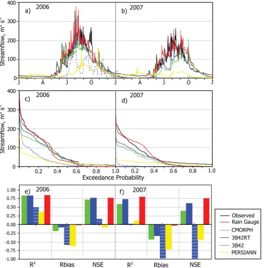
Comparisons of simulated and observed streamflow for the larger watershed, Gilgel Abay, are given in Fig. 5. Let us start with the 2006 results. Figure 5a shows that the

15

3B42, CMORPH and rain gauge simulations capture remarkably the observed stream-flow hydrographs, while the 3B42RT and PERSIANN simulations fail to capture satis-factorily the observed hydrographs resulting in substantial underestimation. Figure 5c shows that all the satellite simulations underestimate the frequency of extreme events; the underestimation is moderate in the case of 3B42RT and CMORPH but severe in

20

the case of 3B42 and PERSIANN simulations; the rain gauge simulation perform very well. Figure 5e shows that theR2values for the time series of daily streamflow between simulated and observed values are higher (0.75) for the 3B42RT, CMORPH and rain gauge simulations compared to the 3B42 (0.50) and PERSIANN (0.37) values. All sim-ulations underestimate the total streamflow volume; the underestimation is negligible

25

for the rain gauges, moderate (Rbias=−0.08,−0.18) for the 3B42RT and CMORPH,

and severe (Rbias=−0.58,−0.62) for the 3B42 and PERSIANN simulations. The NSE

(10)

HESSD

7, 8213–8232, 2010

Title Page

Tables Figures

◭ ◮

Back Close

Full Screen / Esc

Discussion

P

a

per

|

Dis

cussion

P

a

per

|

Discussion

P

a

per

|

Discussio

n

P

a

per

|

low (0.16) for the 3B42, and negative for PERSIANN. The performance accuracy of all satellite simulation is lower in 2007 than it is in 2006; however, the 3B42RT, CMORPH and rain gauge simulations still have modest skills in reproducing daily streamflow, while both 3B42 and PERSIANN show no skills.

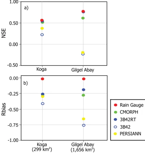
3.3 Koga vs. Gilgel Abay

5

Koga and Gilgel Abay are adjoining watersheds with similar landscape characteristics in similar climates. The major difference between the two is watershed area, Koga at 299 km2 and Gilgel Abay at 1656 km2. Comparison of the performance statistics be-tween the two watersheds reveals the effect of watershed area on the utility of satellite rainfall products as input into SWAT for daily streamflow simulation. Figure 6 presents

10

comparison of the performance statistics (Rbias and NSE) between the two water-sheds, for each rainfall input simulation. Increasing watershed area increases slightly the performance accuracy of the 3B42RT, CMORPH and rain gauge simulations, but decreases substantially the performance accuracy of the 3B42 and PERSIANN sim-ulations. The increased performance accuracy of the 3B42RT, CMORPH and rain

15

gauge simulations for larger watersheds is as expected due to the additional averaging process in larger watersheds that tends to dampen the random error in rainfall input and hydrological process approximation. The decreasing performance accuracy of the 3B42 and PERSIANN in larger watersheds is counter-intuitive and indicates that larger watersheds introduce much more errors from the unreliable rainfall estimates of 3B42

20

and PERSIANN than the reduction in random error gained due to more averaging.

4 Conclusions

The main purpose of this study is to assess the utility of satellite rainfall estimates as input into a hydrological model for daily streamflow simulation in the East African highlands. We limited our analyses to the following specifics: the semi-distributed

(11)

HESSD

7, 8213–8232, 2010

Title Page

Tables Figures

◭ ◮

Back Close

Full Screen / Esc

Discussion

P

a

per

|

Dis

cussion

P

a

per

|

Discussion

P

a

per

|

Discussio

n

P

a

per

|

hydrologic model SWAT; adjoining two watersheds, Koga at 299 km2and Gilgel Abay at 1656 km2; and four types of satellite precipitation products (3B42RT, 3B42, CMORPH, and PERSIANN). Our results reveal that the utility of satellite rainfall products as input to SWAT for daily streamflow simulation strongly depends on the product type. The 3B42RT and CMORPH simulations show consistent and modest skills in their

simu-5

lations but underestimate the large flood peaks. On the other hand, the 3B42 and PERSIANN simulations have inconsistent performance with poor or no skills. Let us put these results in perspective.

Microwave vs. infrared algorithm products

Depending on the main input, satellite rainfall algorithms can be grouped into two

10

categories: those that use primarily microwave data (e.g., CMORPH, 3B42RT) and those that use primarily infrared data (e.g., PERSIANN). The conventional notion is that the microwave-based algorithms fare better than the infrared-based algorithms. Our results indicate that not only are the microwave-based algorithms better than the infrared-based algorithm, but the infrared-based algorithm also has poor or no skills for

15

streamflow simulations. We conclude that the infrared-based algorithm PERSIANN is not a reliable source of rainfall data in the East African highlands.

Satellite-gauge vs. satellite-only products

The conventional notion that the satellite rainfall estimates that incorporate rain gauge information perform better than the satellite-only estimates has led to the incorporation

20

of rain gauge data into global satellite rainfall products. Our results turn this conven-tional notion on its head. The satellite-only product (3B42RT) performs much better than the satellite-gauge product (3B42). Apparently incorporating rain gauge data in satellite rainfall products has the undesirable consequence of deteriorating the quality of the satellite rainfall products in this region. This suggests that the algorithm used

25

(12)

HESSD

7, 8213–8232, 2010

Title Page

Tables Figures

◭ ◮

Back Close

Full Screen / Esc

Discussion

P

a

per

|

Dis

cussion

P

a

per

|

Discussion

P

a

per

|

Discussio

n

P

a

per

|

modified to account for the effects of mountainous topography and sparse rain gauge network.

Effect of watershed area

One would expect the performance accuracy of the satellite streamflow simulations to increase as the watershed area becomes larger. Our results indicate that this actually

5

depends on the satellite rainfall product used as input. For satellite rainfall products that have relatively reliable and consistent performance (3B42RT and CMORPH), the resulting streamflow simulations will indeed have higher performance for larger water-sheds. However, for satellite rainfall products that have unreliable and inconsistent per-formance (3B42 and PERSIANN), the resulting streamflow simulations’ perper-formance

10

accuracy decreases as the watershed area increases from 299 km2 to 1656 km2, in-dicating that larger watersheds introduce more errors from the unreliable rainfall esti-mates of 3B42 and PERSIANN than the reduction in random error gained due to more averaging.

Acknowledgements. Support for this study came from two NASA Grants (Award #:

15

NNX08AR31G and NNX10AG77G) to the University of Connecticut.

References

Arnold, J. G., Srinivasan, R., Muttiah, R. S., and Allen, P. M.: Large-Area Hydrologic Modeling and Asssessment: Part I. Model Development, J. Amer. Water Resour. Assoc., 34(1), 73–89, doi:10.1111/j.1752-1688.1998.tb05961.x, 1998.

20

Eckhardt, K. and Arnold, J. G.: Automatic calibration of a distributed catchment model, J. Hydrol., 251(1–2), 103–109, doi:10.1016/S0022-1694(01)00429-2, 2001.

Gassman, P. W., Reyes, M. R., Green, C. H., and Arnold, J. G.: The soil and water assessment tool: Historical development, applications, and future research directions, Trans. ASABE, 50(4), 1211–1250, 2007.

(13)

HESSD

7, 8213–8232, 2010

Title Page

Tables Figures

◭ ◮

Back Close

Full Screen / Esc

Discussion

P

a

per

|

Dis

cussion

P

a

per

|

Discussion

P

a

per

|

Discussio

n

P

a

per

|

Huffman, G. J., Adler, R. F., Bolvin, D. T., Gu, G., Nelkin, E. J., Bowman, K. P., Hong, Y., Stocker, E. F., and Wolff, D. B.: The TRMM Multisatellite Precipitation Analysis (TMPA): Quasi-global, multilayer, combined-sensor, precipitation estimates at fine scale, J. Hydrometeorol., 8, 38– 55, 2007.

Joyce, R. J., Janowiak, J. E., Arkin, P. A., and Xie, P.: CMORPH: A method that produces 5

global precipitation estimation from passive microwave and infrared data at high spatial and temporal resolution, J. Hydrometeorol., 5, 487–503, 2004.

Kidd, C. and Muller, C.: The combined passive microwave-infrared (PMIR) algorithm, in: Satel-lite Rainfall Applications for Surface Hydrology, edited by: Gebremichael, M. and Hossain, F., Springer-Verlag, doi:10.1007/978-90-481-2915-7 5, 2009.

10

Legates, D. R. and McCabe, G. J.: Evaluating the use of “goodness of fit” measures in hydro-logic and hydroclimatic model validation, Water Resour. Res., 35(1), 233–241, 1999. Scofield, R. A. and Kuligowski, R. J.: Status and outlook of operational satellite precipitation

algorithms for extreme-precipitation events, Weather Forecast., 18, 1037–1051, 2003. Soil Conservation Service: TR-55, Urban Hydrology for Small Watersheds, Natural Resources 15

Conservation Service, Washington, DC, 1986.

Sorooshian, S., Hsu, K., Gao, X., Gupta, H. V., Imam, B., and Braithwaite, D.: Evaluation of PERSIANN system satellite-based estimates of tropical rainfall, B. Am. Meteor. Soc., 81, 2035–2046, 2000.

Turk, F. J. and Miller, S. D.: Toward improved characterization of remotely sensed precipitation 20

regimes with MODIS/AMSR-E blended data techniques, IEEE T. Geosci. Remote, 43, 1059– 1069, 2005.

Ushio, T. and Kachi, M.: Kalman filtering applications for global satellite mapping of precipitation (GSMaP), in: Satellite Rainfall Applications for Surface Hydrology, edited by: Gebremichael, M. and Hossain, F., Springer-Verlag, doi:10.1007/978-90-481-2915-7 7, 2009.

25

(14)

HESSD

7, 8213–8232, 2010

Title Page

Tables Figures

◭ ◮

Back Close

Full Screen / Esc

Discussion

P

a

per

|

Dis

cussion

P

a

per

|

Discussion

P

a

per

|

Discussio

n

P

a

per

|

Table 1.SWAT model parameter estimates for each watershed and rainfall input source.

Parameter Model parameter Variable Unit Parameter values for Koga (Gilgel Abay)

type

Routing Hydraulic conductivity of CH K2 mm 1.1 23.6 29.3 143.7 0.01

main channel alluvium hr−1 (60) (60) (60) (60) (60)

Ground Base flow alpha factor Alpha BF day−1 0.97 0.97 0.97 0.97 0.97

water (0.75) (0.75) (0.75) (0.75) (0.75)

HRU Curve number CN2* – 62 69 69 73 72

(50) (57) (57) (72) (67)

Basin Surface runofflag Surlag – 0.001 0.001 0.001 8.94 0.001

coefficient (8) (8) (8) (8) (0.1)

Routing Manning’s “n” value for CH N2 – 0.04 0.02 0.01 0.06 0.116

main channel (0.04) (0.04) (0.04) (0.04) (0.04)

HRU Soil hydraulic conductivity Sol K* mm 0.02 0.02 0.02 0.02 0.02

hr−1 (0.0175) (0.0175) (0.0175) (0.0175) (0.0175)

HRU soil evaporation ESCO 0.92 1 0.99 1 1

compensation factor (0) (0) (0) (0) (0)

HRU Maximum canopy storage canmx – 2.34 2.34 1.44 0 0.39

(2.5) (0) (0) (0) (0)

Ground Deep aquifer percolation Rchrg dp – 0.01 0.01 0.01 0.01 0.01

water fraction (0.25) (0) (0) (0) (0)

Ground Groundwater delay Gw delay day 31 31 31 31 31

water (25) (25) (25) (25) (25)

Ground Threshold depth of water Gwqmn mm 0 0 0 0 0

water in the shallow (1500) (0) (0) (0) (0)

aquifer for return flow to occur

(15)

HESSD

7, 8213–8232, 2010

Title Page

Tables Figures

◭ ◮

Back Close

Full Screen / Esc

Discussion

P

a

per

|

Dis

cussion

P

a

per

|

Discussion

P

a

per

|

Discussio

n

P

a

per

|

10 km

Satellite Rainfall Grid

Elevation, m

3,530

1,885

Gilgel Abay

Koga

(37° 30' 00", 11° 30' 00") 0.25°

0.25

°

.

&

3

&

3

&

3

&

3

&

3

X X

Stream Gauge Station Rain Gauge Station X

Fig. 1. The study region in Ethiopian highlands consisting of two adjoining watersheds: Koga (299 km2) and Gilgel Abay (1656 km2). Also shown are satellite rainfall grids (0.25◦

×0.25◦) and

(16)

HESSD

7, 8213–8232, 2010

Title Page

Tables Figures

◭ ◮

Back Close

Full Screen / Esc

Discussion

P

a

per

|

Dis

cussion

P

a

per

|

Discussion

P

a

per

|

Discussio

n

P

a

per

|

a) 2003 2004

0 20 40 60

3B42RT 3B42 Observed

CMORPH

PERSIANN b)

Koga

c) 2003 2004

J A J O J A J O J

Streamflow, m

3

s

-1

0 100 200 300 400

d)

Gilgel Abay

Rain Gauge

(17)

HESSD

7, 8213–8232, 2010

Title Page

Tables Figures

◭ ◮

Back Close

Full Screen / Esc

Discussion

P

a

per

|

Dis

cussion

P

a

per

|

Discussion

P

a

per

|

Discussio

n

P

a

per

|

CMORPH Rainfall 3B42RT Rainfall 3B42 Rainfall PERSIANN Rainfall Rain Gauge Rainfall

0 500 1000 1500 2000 2500

Observed Streamflow

a) b)

Koga Gilgel Abay

2003 2004 2003 2004

3000

Depth, mm

(18)

HESSD

7, 8213–8232, 2010

Title Page

Tables Figures

◭ ◮

Back Close

Full Screen / Esc

Discussion

P

a

per

|

Dis

cussion

P

a

per

|

Discussion

P

a

per

|

Discussio

n

P

a

per

|

2006 2007

J A J O J A J O J

0 20 40 60

1.0 0.8 0.6 0.4

0.2 0.2 0.4 0.6 0.8 1.0

Exceedance Probability

2006 2007

-1.00 -0.75 -0.50 -0.25 0.00 0.25 0.50 0.75 1.00

Rbias NSE

R2 R2 Rbias NSE

2006 2007

Streamflow, m

3

s

-1

0 20 40 60

Streamflow, m

3

s

-1

a)

c)

e)

b)

d)

f)

Koga Validation (2006-2007)

3B42RT 3B42 Observed

CMORPH

PERSIANN Rain Gauge

(19)

HESSD

7, 8213–8232, 2010

Title Page

Tables Figures

◭ ◮

Back Close

Full Screen / Esc

Discussion

P

a

per

|

Dis

cussion

P

a

per

|

Discussion

P

a

per

|

Discussio

n

P

a

per

|

2006 2007

J A J O J A J O J

1.0 0.8 0.6 0.4

0.2 0.2 0.4 0.6 0.8 1.0

Exceedance Probability

2006 2007

-1.00 -0.75 -0.50 -0.25 0.00 0.25 0.50 0.75 1.00

Rbias NSE

R2 R2 Rbias NSE

2006 2007

Streamflow, m

3

s

-1

Streamflow, m

3

s

-1

0 100 200 300 400 0 100 200 300 400

a)

d)

e) c)

b)

3B42RT 3B42 Observed Rain Gauge CMORPH

PERSIANN f)

Gilgel Abay Validation (2006-2007)

(20)

HESSD

7, 8213–8232, 2010

Title Page

Tables Figures

◭ ◮

Back Close

Full Screen / Esc

Discussion

P

a

per

|

Dis

cussion

P

a

per

|

Discussion

P

a

per

|

Discussio

n

P

a

per

|

-0.75 0.00

-1.00 -0.50 -0.25 -0.50 0.00 0.50 1.00

a)

b)

Gilgel Abay Koga

(299 km2) (1,656 km2)

Rbias

N

SE

3B42RT

3B42 CMORPH

PERSIANN Rain Gauge