Evaluation of an extreme-condition-inverse calibration remote sensing model for mapping energy balance fluxes in arid riparian areas

(1)

HESSD

11, 13479–13539, 2014

Mapping energy balance fluxes in arid

riparian areas

S.-H. Hong et al.

Title Page

Abstract Introduction

Conclusions References

Tables Figures

◭ ◮

Back Close

Full Screen / Esc

Printer-friendly Version

Interactive Discussion

Discussion

P

a

per

|

Discussion

P

a

per

|

Discussion

P

a

per

|

Discussion

P

a

per

|

Hydrol. Earth Syst. Sci. Discuss., 11, 13479–13539, 2014 www.hydrol-earth-syst-sci-discuss.net/11/13479/2014/ doi:10.5194/hessd-11-13479-2014

This discussion paper is/has been under review for the journal Hydrology and Earth System Sciences (HESS). Please refer to the corresponding final paper in HESS if available.

Evaluation of an

extreme-condition-inverse calibration

remote sensing model for mapping

energy balance fluxes in arid riparian

areas

S.-H. Hong1,*, J. M. H. Hendrickx1, J. Kleissl2, R. G. Allen3,

W. G. M. Bastiaanssen4, R. L. Scott5, and A. L. Steinwand6

1

New Mexico Tech, Socorro, NM, USA

2

University of California, San Diego, CA, USA

3

University of Idaho, Kimberly, ID, USA

4

Delft University of Technology, Delft, the Netherlands

5

Southwest Watershed Research Center, USDA-ARS, Tucson, AZ, USA

6

Inyo County, Water Department, Independence, CA, USA

*

(2)

HESSD

11, 13479–13539, 2014

riparian areas

S.-H. Hong et al.

Title Page

Tables Figures

◭ ◮

Back Close

Full Screen / Esc

Discussion

P

a

per

|

Discussion

P

a

per

|

Discussion

P

a

per

|

Discussion

P

a

per

|

Received: 22 August 2014 – Accepted: 17 November 2014 – Published: 10 December 2014 Correspondence to: S.-H. Hong (shong4@murraystate.edu)

(3)

HESSD

11, 13479–13539, 2014

riparian areas

S.-H. Hong et al.

Title Page

Tables Figures

◭ ◮

Back Close

Full Screen / Esc

Discussion

P

a

per

|

Discussion

P

a

per

|

Discussion

P

a

per

|

Discussion

P

a

per

|

Abstract

Accurate information on the distribution of the surface energy balance components in arid riparian areas is needed for sustainable management of water resources as well as for a better understanding of water and heat exchange processes between the land surface and the atmosphere. Since the spatial and temporal distributions of these fluxes

5

over large areas are difficult to determine from ground measurements alone, their pre-diction from remote sensing data is very attractive as it enables large area coverage and a high repetition rate. In this study the Surface Energy Balance Algorithm for Land (SEBAL) was used to estimate all the energy balance components in the arid riparian areas of the Middle Rio Grande Basin (New Mexico), San Pedro Basin (Arizona), and

10

Owens Valley (California). We compare instantaneous and daily SEBAL fluxes derived from Landsat TM images to surface-based measurements with eddy covariance flux towers. This study presents evidence that SEBAL yields reliable estimates for actual evapotranspiration rates in riparian areas of the southwestern United States. The great strength of the SEBAL method is its internal calibration procedure that eliminates most

15

of the bias in latent heat flux at the expense of increased bias in sensible heat flux.

1 Introduction

The regional distribution of the energy balance components, net surface radiation (Rn), soil heat flux (G), sensible heat flux (H) and latent heat flux (LE) in arid riparian areas is critical knowledge for agricultural, hydrological and climatological investigations.

How-20

ever,Rn,G,Hand LE are complex functions of atmospheric conditions, land use, vege-tation, soils, and topography which cause these fluxes to vary in space and time. There-fore, it is difficult to estimate them at the regional scale (Parlange et al., 1995). Mea-surement approaches for LE from the land surface including eddy covariance (Kizer and Elliott, 1991), Bowen ratio (Scott et al., 2004) and weighing lysimeters (Wright,

25

(4)

HESSD

11, 13479–13539, 2014

riparian areas

S.-H. Hong et al.

Title Page

Tables Figures

◭ ◮

Back Close

Full Screen / Esc

Discussion

P

a

per

|

Discussion

P

a

per

|

Discussion

P

a

per

|

Discussion

P

a

per

|

spatial density at the regional scale. These techniques produce LE measurements over small footprints (m2to ha) which are difficult to extrapolate to the regional scale, especially over heterogeneous land surfaces (Moran and Jackson, 1991). For example, in the heterogeneous landscape of the central plateau of Spain as many as 13 ground measurements of evapotranspiration in a relatively small area of 5000 km2 were not

5

sufficient to predict accurately the area-averaged evapotranspiration rate (Pelgrum and Bastiaanssen, 1996).

Reliable regional estimates of spatial patterns of LE can only be obtained by satellite image-based remote sensing algorithms as has been shown by a number of investi-gators (e.g. Choudhury, 1989; Granger, 2000; Moran and Jackson, 1991; Kustas and

10

Norman, 1996; Du et al., 2013). Today a variety of LE remote sensing algorithms ex-ists with di_fferent spatial (30 m to 1/8◦_{or 13 km in New Mexico) and temporal (daily to}

monthly) scales: the North American Land Data Assimilation Systems (NLDAS) (Cos-grove et al., 2003), the Land Information Systems (LIS) (Peters Lidard et al., 2004), the Two-Source Energy Balance model (TSEB) (Norman et al., 1995), the Hybrid

15

dual source Trapezoid framework Evapotranspiration Model (HTEM) (Yang and Shang, 2013), the Atmosphere–Land Exchange Inverse (ALEXI) (Anderson et al., 1997), the disaggregated ALEXI model (DisALEXI) (Norman et al., 2003), the Surface Energy Balance System (SEBS) (Su, 2002), the MOD16 ET algorithms (Mu et al., 2011), the Simplified Surface Energy Balance (SSEB) (Senay et al., 2013), the Surface Energy

20

Balance Algorithm for Land (SEBAL) (Bastiaanssen, 1995), Mapping EvapoTranspi-ration at high spatial Resolution with Internalized CalibEvapoTranspi-ration (METRIC) (Allen et al., 2007), as well as algorithms without distinct acronyms (Schüttemeyer et al., 2007; Ma et al., 2004; Jiang and Islam, 2001).

SEBAL has been developed and pioneered by Bastiaanssen and his colleagues in

25

(5)

HESSD

11, 13479–13539, 2014

riparian areas

S.-H. Hong et al.

Title Page

Tables Figures

◭ ◮

Back Close

Full Screen / Esc

Discussion

P

a

per

|

Discussion

P

a

per

|

Discussion

P

a

per

|

Discussion

P

a

per

|

region of interest; unlike NLDAS and LIS, SEBAL and METRIC do not require land cover maps. However, applications of SEBAL and METRIC are restricted to clear days over areas of unvarying weather, and require some supervised calibration for each image, preventing application at the continental scale such as done by ALEXI, SSEB, MOD16, NLDAS and LIS.

5

The accuracy of SEBAL and METRIC for evaporation mapping worldwide is typi-cally about±15 and±5 % for, respectively, daily and seasonal evaporation estimates (Bastiaanssen et al., 2005; Allen et al., 2011). Such accuracy is obtained by a cali-bration method that selects a “cold” and “hot” pixel representing extreme thermal and vegetation conditions within an image. After calculation of the energy balance at the

10

two calibration pixels the sensible heat flux H for each pixel is indexed to its satellite measured surface temperature. The economic efficiency of SEBAL and METRIC is re-markable. For example, in the early 1980’s co-author Hendrickx was deployed at Niono in the O_ffice du Niger in Mali to determine water requirements for flood irrigated rice. It took him and a team of four field assistants and several graduate students more than

15

two years to measure the seasonal actual evapotranspiration of rice in four irrigation units covering a total area of about 70 ha using non-weighing lysimeters and discharge measurement structures in irrigation and drainage ditches (Hendrickx et al., 1986). In 2008, the seasonal actual evapotranspiration was obtained for all 86 000 ha of the Of-fice du Niger using SEBAL with Landsat imagery of 2006 at an e_ffort of about two

20

expert months without need for an overseas multi-year deployment (Zwart and Leclert, 2010).

Previous validation studies of SEBAL have mainly been conducted in relatively ho-mogeneous agricultural areas and have focused on comparison of daily ET rates esti-mated from SEBAL and METRIC with ground measurements using lysimeters (Tasumi,

25

(6)

HESSD

11, 13479–13539, 2014

riparian areas

S.-H. Hong et al.

Title Page

Tables Figures

◭ ◮

Back Close

Full Screen / Esc

Discussion

P

a

per

|

Discussion

P

a

per

|

Discussion

P

a

per

|

Discussion

P

a

per

|

in New Mexico, Arizona and California. Here, vast deserts are transected by narrow river valleys covered by a mosaic of irrigated agricultural fields and riparian vegeta-tion (cottonwood, saltcedar, willow, mesquite, Russian olive and salt grasses) which creates a very heterogeneous landscape with a short patch length scale. If SEBAL performs well under these challenging conditions, it is likely to perform well in most

5

arid and semi-arid regions. Another difference with previous studies is our focus on all components of the energy balance during the instant of satellite overpass as well as on a daily basis. We can accomplish this since we have available a quality controlled data set consisting ofRn,H and LE measurements in the riparian areas of the Middle Rio Grande Basin (New Mexico) and R_n,G,H and LE measurements in the riparian

10

areas of the San Pedro Basin (Arizona) and the Owens River Valley (California).

2 Surface Energy Balance Algorithm for Land (SEBAL)

SEBAL is a remote sensing algorithm that evaluates the fluxes of the energy balance and determines LE as the residual

LE=Rn−G−H (1)

15

whereRnis the net radiation flux density [W m− 2

],Gis the soil heat flux density [W m−2], His the sensible heat flux density [W m−2], and LE (=λET) is the latent heat flux density [W m−2

], which can be converted to the ET rate [mm day−1

] using the latent heat of vaporization of waterλ[J kg−1] and the density of waterρw[kg m−

3 ].

To implement SEBAL, images are needed with information on reflectance in the

vis-20

ible, near-infrared and mid-infrared bands as well as emission in the thermal infrared band. Such images are offered by a number of satellites such as Land Satellite (Land-sat), Moderate Resolution Imaging Spectroradiometer (MODIS), Advanced Very High Resolution Radiometer (AVHRR), Advanced Spaceborne Thermal Emission and Re-flection Radiometer (ASTER), ENVISAT-Advanced Along Track Scanning Radiometer

(7)

HESSD

11, 13479–13539, 2014

riparian areas

S.-H. Hong et al.

Title Page

Tables Figures

◭ ◮

Back Close

Full Screen / Esc

Discussion

P

a

per

|

Discussion

P

a

per

|

Discussion

P

a

per

|

Discussion

P

a

per

|

(AATSR) and China–Brazil Earth Resources Satellite (CBERS). In this study, we use Landsat images for their high spatial resolution. In undulated landscapes and moun-tains, a Digital Elevation Model (DEM) is also needed to take into account terrain slope and aspect of each pixel. Extensive descriptions of SEBAL and METRIC have been presented in the literature (Bastiaanssen et al., 1998a; Hong, 2008; Allen et al., 2007).

5

Therefore, we refer to these publications and the PhD dissertation by Hong (2008) for the full details of our SEBAL implementation. Here below we only discuss a critical portion of the SEBAL algorithm.

Rn and G are determined using standard approaches similar to other LE remote sensing algorithms but SEBAL and METRIC have a different unique method for the

10

estimation of the sensible heat flux densityH defined as (Brutsaert et al., 1993)

H=ρa·cp·(T_r aero−Ta) ah

(2)

whereρais the density of air [kg m− 3

],cpis the specific heat capacity of air [J kg−1K−1],

Taero is the aerodynamic surface temperature, Ta is the air temperature measured at a standard screen height, andrahis the aerodynamic resistance to heat transfer [s m−

1 ].

15

SEBAL and METRIC overcome the challenge of inferring the aerodynamic surface temperature from the radiometric surface temperature and the need for near-surface air temperature measurements by directly estimating the temperature difference ∆T betweenT1andT2taken at two levelsz1(0.10 m) andz2(2 m) above the canopy or soil surface without calculation of the absolute temperature at a given height.

20

H=ρa·cp·∆T

rah12

(3)

(8)

HESSD

11, 13479–13539, 2014

riparian areas

S.-H. Hong et al.

Title Page

Tables Figures

◭ ◮

Back Close

Full Screen / Esc

Discussion

P

a

per

|

Discussion

P

a

per

|

Discussion

P

a

per

|

Discussion

P

a

per

|

(Eq. 1) with LE set to zero so that H=Rn−G followed by the inversion of Eq. (3) to ∆T =Hrah12/(ρacp). On the other hand, for a wet surface (the “cold” pixel) all available

energyRn−Gis assumed in traditional applications of SEBAL to be used for evapotran-spiration so thatH=0 and∆T =0 (Bastiaanssen et al., 1998a; Bastiaanssen, 2000). The implicit assumption in extreme-condition-inverted-calibration processes such as

5

SEBAL and METRIC is that land surfaces with a high ∆T are associated with high radiometric temperatures and those with a low∆T with low radiometric temperatures. Field measurements in Egypt and Niger (Bastiaanssen et al., 1998b), China (Wang et al., 1998), and USA (Franks and Beven, 1997) have shown that the relationship be-tweenT_sand∆T is approximately positively linear for different field conditions including

10

irrigated fields, deserts and mountains.

∆T =c1·Ts+c2 (4)

wherec1andc2are the linear regression coefficients valid for a landscape at the time and date the image is taken. By using the values of ∆T calculated for the cold and hot pixel the regression coefficientsc1andc2can be determined so that the extremes

15

ofH are constrained and outliers ofH-fluxes are prevented. The Eq. (4) is dependent upon spatial differences of the radiometric surface temperature rather than absolute surface temperatures to derive maps of the sensible heat flux which minimizes the need for atmospheric corrections as well as uncertainties in surface emissivity, surface roughness and differences inTaeroandTsonH estimates (Allen et al., 2007).

20

Besides∆T the other unknown in Eq. (3) is the aerodynamic resistance to heat trans-ferrah12which is affected by wind speed, atmospheric stability, and surface roughness. Sincerah12is needed to calculateH whileH is required to calculaterah12, an iterative process is used to findH (Allen et al., 2007; Hong, 2008). Then, after insertingRn,G andH into Eq. (1) the latent heat flux LE is obtained for each pixel. Finally, dividing LE

25

(9)

HESSD

11, 13479–13539, 2014

riparian areas

S.-H. Hong et al.

Title Page

Tables Figures

◭ ◮

Back Close

Full Screen / Esc

Discussion

P

a

per

|

Discussion

P

a

per

|

Discussion

P

a

per

|

Discussion

P

a

per

|

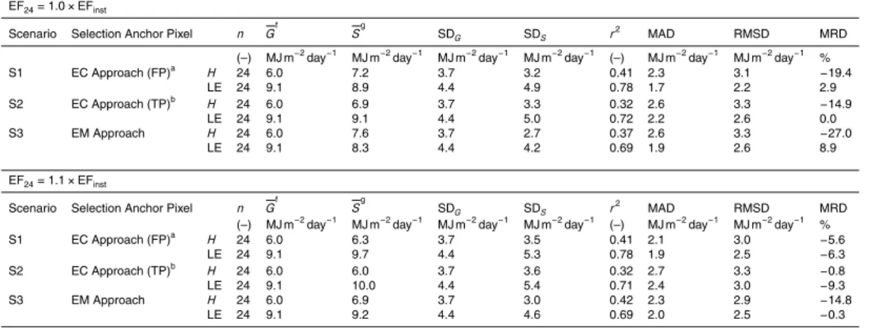
SEBAL produces an estimate of the instantaneous LE at the time of the satellite overpass. However, for most hydrological applications the daily LE is needed; so the instantaneous LE needs to be extrapolated to the daily LE which is done using the instantaneous evaporative fraction (EF_inst). Where soil moisture does not significantly change and advection does not occur, the evaporative fraction has been shown to be

5

approximately constant during the day (Crago, 1996; Farah et al., 2004). However, analysis of field measurements by other investigators (Teixeira et al., 2008; Anderson et al., 1997; Sugita and Brutsaert, 1991) indicates that the instantaneous evaporative fraction on clear days at satellite overpass time (around 10:30 a.m.) tends to be approx-imately 10–18 % smaller than the daytime average. Therefore, a correction coefficient

10

cEF is introduced to take into account differences between instantaneous and daily evaporative fractions. Some investigators usecEF of 1.00 (Bastiaanssen et al., 2005) while otherssuggestcEF of 1.10 (Anderson et al., 1997) orcEF of 1.18 (Teixeira et al., 2008). The value forcEF should depend on the relative amount of advection of heat, which in turn is a function of regional evaporation, wind speed and relative humidity.

15

EFinst·cEF=

Rn−G−H Rn−G

·cEF=

LEinst LEinst+Hinst

·cEF=EF24 (5)

AssumingcEF of 1.0 and daily soil heat fluxG24 [MJ m− 2

day−1_{] close to zero,}

multipli-cation of the instantaneous EFinstdetermined from SEBAL with the total daily available energy yields the daily ET rate in mm per day (Bastiaanssen et al., 1998a) as

ET₂₄=EFinst·(Rn24−G24)

λ·ρw

≈EF24·Rn24 λ·ρw

(6)

20

where ET24 is daily ET [mm day− 1

], ρw is the density of water [kg m− 3

(10)

HESSD

11, 13479–13539, 2014

riparian areas

S.-H. Hong et al.

Title Page

Tables Figures

◭ ◮

Back Close

Full Screen / Esc

Discussion

P

a

per

|

Discussion

P

a

per

|

Discussion

P

a

per

|

Discussion

P

a

per

|

3 Method and materials

3.1 Study areas

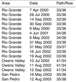
The components of the energy balance (Rn,G,H and LE) are determined by SEBAL from sixteen Landsat 7 images of year 2000 to 2003 for three typical riparian areas in the southwestern United States located in the Middle Rio Grande Valley (NM), the

5

Owens Valley (CA) and the San Pedro Basin (AZ) (Table 1).

The Middle Rio Grande Valley extends through central New Mexico and is defined as the reach of the Rio Grande between Cochiti Dam and Elephant Butte Reservoir. The Middle Rio Grande riparian vegetation consists of cottonwood and salt grasses as well as various non-native species including saltcedar and russian olive. In the Middle Rio

10

Grande Valley, the average annual air temperature is 15◦C. Daily summer temperatures range from 20 to 40◦_{C, while daily winter temperatures range from}

−12 to 10◦C. Mean annual precipitation is about 25 cm and mean annual potential evapotranspiration is approximately 170 cm.

The Owens Valley is a long, narrow valley on the eastern slope of the Sierra Nevada

15

in Inyo County, California. It is a closed basin drained by the Owens River which ter-minates at saline Owens Lake. The Owens Valley has a mild high-desert climate: in summer (June, July and August) the lowest average daily minimum temperature is 7◦_C

and the highest average daily maximum temperature temperatures is 37◦C, and in win-ter (November to February) from−7 to 21◦C. Since, the Owens Valley is located in the

20

“rain shadow” of the Sierra Nevada, the average annual precipitation in the Owens Val-ley is only about 12 cm and mean annual potential evapotranspiration is about 150 cm. Snowmelt runofffrom the Sierra Nevada creates a shallow water table underneath the valley floor which supports approximately 28 000 ha of native shrubs and grasses in riparian areas.

25

(11)

HESSD

11, 13479–13539, 2014

riparian areas

S.-H. Hong et al.

Title Page

Tables Figures

◭ ◮

Back Close

Full Screen / Esc

Discussion

P

a

per

|

Discussion

P

a

per

|

Discussion

P

a

per

|

Discussion

P

a

per

|

Upper San Pedro valley is around 18◦_{C. Daily summer temperatures range from 22 to}

44◦C, while daily winter temperatures range from 9 to 24◦C. Mean annual precipitation is about 35 cm and mean annual potential evapotranspiration is approximately 170 cm. Although, the regional climate of all three areas is classified as arid/semiarid, there exists a difference in precipitation pattern. In the Owens Valley, precipitation occurs

pri-5

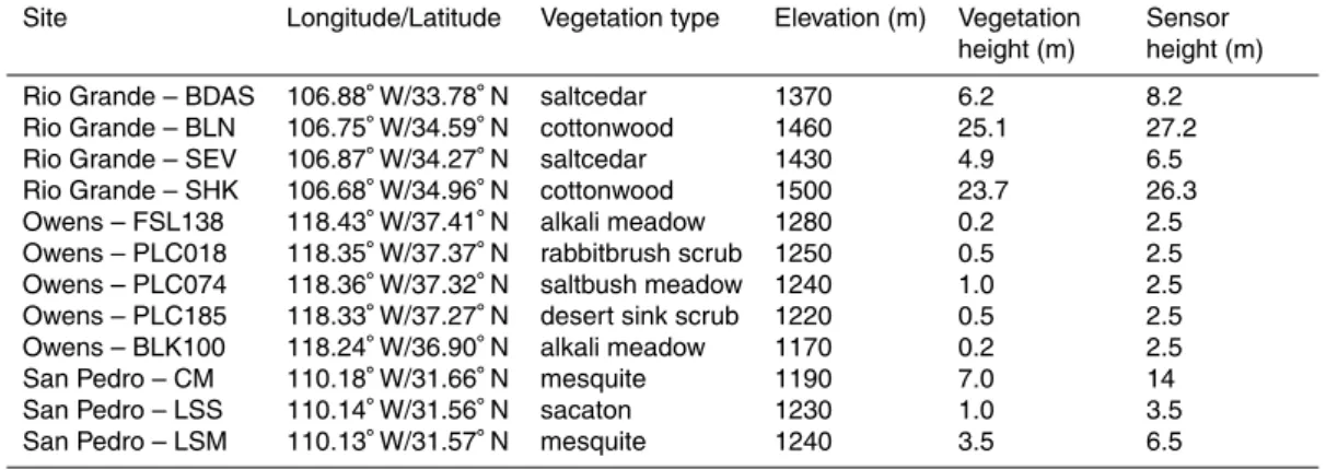
marily in winter and spring, while in the San Pedro and the Middle Rio Grande Valleys, the annual precipitation distribution is bimodal, with more than half of the rainfall being monsoonal in summer, although the proportion varies considerably from year to year (Cleverly et al., 2002; Elmore et al., 2002; Scott et al., 2000; Stromberg, 1998; Costi-gan et al., 2000). Table 2 presents main characteristics of the study sites: vegetation

10

type, elevation above sea level, height of vegetation canopy and the height of flux sen-sors above ground level. The average elevations are 1440, 1230 and 1220 m above sea level for, respectively, the Middle Rio Grande Basin, Owens Valley and San Pedro Valley.

3.2 Eddy covariance measurements and closure forcing

15

SEBAL estimates of LE, H, G, and Rn are compared to ground-based eddy covari-ance and energy balcovari-ance measurements. At each site, the turbulent heat fluxes were measured using the eddy covariance (EC) method that theoretically provides direct and reliable measurements ofH and LE (Arya, 2001). At all sites, a three-dimensional sonic anemometer-thermometer that measures the three-dimensional wind vector and

20

virtual temperature, was collocated with a Krypton hygrometer or open path infrared gas analyzer that measures water vapor density [g m−3] with a sampling rate of 10 Hz (Cleverly et al., 2002; Steinwand et al., 2006; Scott et al., 2004). The covariances be-tween the vertical wind speed and, respectively, water vapor density and virtual air temperature are used for the computation of, respectively, 30 min averages of the

la-25

(12)

HESSD

11, 13479–13539, 2014

riparian areas

S.-H. Hong et al.

Title Page

Tables Figures

◭ ◮

Back Close

Full Screen / Esc

Discussion

P

a

per

|

Discussion

P

a

per

|

Discussion

P

a

per

|

Discussion

P

a

per

|

controlled and corrected for tilt by coordinate rotations, frequency response, oxygen absorption of the Krypton hygrometer, and flux effects on air density. The coordinate rotation, however, cannot correct for effects of changing wind direction during 30 min average periods that can cause mean “vertical” wind speeds to deviate from 0, thereby inducing error in theH and LE measurements. This problem is common to EC

mea-5

surements in tall vegetation such as trees where the sensors are placed too close to tree branches or canopy. Soil heat fluxes in the San Pedro Valley and Owens Valley were obtained from measurements using soil heat flux plates that were corrected for soil heat storage above the plate using collocated soil temperature and soil moisture measurements.

10

At the Middle Rio Grande sites, soil heat storage could not be calculated due to the absence of soil moisture measurements. Therefore, the soil heat flux measurements in the Middle Rio Grande Valley have not been compared with those estimated by SEBAL. The net radiation was obtained from REBS Q7 or Kipp and Zonen CNR1 net radiome-ters. In some of the installations, the Rn sensors may have been mounted too close

15

to the towers and may have been impacted by reflection from the local structure. For the comparison of the 30 min averaged ground measurements with the instantaneous energy fluxes estimated using SEBAL, an “instantaneous” ground measurement was determined by linear interpolation between the two 30 min averaged, ground measure-ments before and after the satellite overpass. To compute daily values of LE,H,Gand

20

Rnthe 30 min flux data were summed over the day (00:00–24:00 LT).

We use the relative closure of the energy balance (Twine et al., 2000) as a criterion for the selection of high-qualityRn,G,H, and LE ground measurements for comparison with SEBAL estimates. Figure 1 presents the relative closures calculated for satellite overpass days for all sites as provided by the investigators operating the EC towers

25

(13)

rea-HESSD

11, 13479–13539, 2014

riparian areas

S.-H. Hong et al.

Title Page

Tables Figures

◭ ◮

Back Close

Full Screen / Esc

Discussion

P

a

per

|

Discussion

P

a

per

|

Discussion

P

a

per

|

Discussion

P

a

per

|

sonable agreement found between SEBAL derived instantaneous soil heat fluxes and those measured on the ground in the Owens and San Pedro River Valleys (Table 5). If the sum ofH and LE, before correction, was less than 65 % or greater than 110 % of the available energy (Rn−G), the data were not used in our analysis. This criterion

leads to the exclusion of 45 % of instantaneous fluxes and 39 % of the daily fluxes of

5

the data from the Middle Rio Grande Valley, 79 % (instantaneous) and 43 % (daily) from the Owens River Valley and 17 % (instantaneous) and zero % (daily) from the San Pe-dro River Valley. The remaining turbulent heat flux estimates are improved thru forcing the closure of the energy balance by increasing LE andH by the Bowen ratio (Twine et al., 2000). The improved adjustedH and LE are identified asH_adjand LE_adj.

10

After elimination of EC measurements on the basis of unacceptable closures, we eliminated also the EC measurements taken on 16 May 2003 in the San Pedro River Valley at the Mesquite (CM) site. On this day the wind direction was approximately 90◦ di_fferent from the prevailing wind direction which resulted in fetch distances consid-erably shorter than the recommended 100 times the sensor height above the canopy

15

(Stannard, 1993; Sumner and Jacobs, 2005). The problem was exacerbated by the rel-atively high placement (7 m) of the sensors above the canopy (Table 2) since the heat fluxes can vary significantly with height under such conditions (De Bruin et al., 1991).

3.3 Comparison of SEBAL flux predictions to ground measurements

Comparison of SEBAL derived estimates ofRn,G, H and LE with ground

measure-20

ments is not a straightforward operation because the spatial and temporal scales of the SEBAL predictions and ground measurements are quite different. In this section we will discuss these scale gaps for each flux in the energy balance.

3.3.1 Net radiation

Rn is measured with a net radiometer at a height of about 2–3 m above the canopy

25

(14)

measure-HESSD

11, 13479–13539, 2014

riparian areas

S.-H. Hong et al.

Title Page

Tables Figures

◭ ◮

Back Close

Full Screen / Esc

Discussion

P

a

per

|

Discussion

P

a

per

|

Discussion

P

a

per

|

Discussion

P

a

per

|

ments are taken every second and made available as 30 min averages for this study. The SEBALRn prediction is derived from reflectances in the visible, near-infrared and mid-infrared bands from a 900 m2 pixel as well as the emittance in the thermal band from a 3600 m2 pixel. Thus, the Rn ground observation is based on a measurement area at least two orders of magnitude smaller than the SEBAL prediction. For

homo-5

geneous areas this difference will not matter much but for heterogeneous areas it may cause serious bias, since the satellite basedRn samples a larger area and is there-fore more representative of the EC footprint. In riparian areas heterogeneity is the rule rather than exception. Radiometers are typically placed over the canopy of interest which may cause under-representation of surrounding bare soil or ground cover in the

10

angle of view. Therefore, ground measuredRnis expected to be biased towards theRn of the vegetation of interest.

3.3.2 Soil heat flux

Gis measured by soil heat flux plates combined with the determination of changes in heat storage above the plate using soil temperature and soil water content

measure-15

ments. If G is not corrected for heat storage above the plate, large errors will result (Sauer, 2002a). This is the case for the measurements at the Middle Rio Grande sites and, therefore, theseG measurements have not been used for the comparison. The measurement area of a soil heat flux plate is about 0.001 m2 which is almost six or-ders of magnitude less than a 900 m2 Landsat pixel. G is spatially variable due to

20

heterogeneity in soil moisture and vegetation cover, so that numerous flux measure-ments would be needed to estimate the average pixel G with the desired accuracy (Kustas et al., 2000; Humes et al., 1994). Therefore, we expect the instantaneous G ground measurements to be a rather crude estimation of the true instantaneous G of a pixel. The instantaneous G can vary widely depending on soil condition (20–

25

(15)

HESSD

11, 13479–13539, 2014

riparian areas

S.-H. Hong et al.

Title Page

Tables Figures

◭ ◮

Back Close

Full Screen / Esc

Discussion

P

a

per

|

Discussion

P

a

per

|

Discussion

P

a

per

|

Discussion

P

a

per

|

balance (Seguin and Itier, 1983). G is measured in the field every second; we used averages of 30 min for this study.

3.3.3 Sensible and latent heat fluxes

H and LE are measured using a three-dimensional sonic anemometer-thermometer and Krypton hygrometer, respectively (or open patch infrared gas analyzer). For these

5

components of the energy balance the relationship between ground measurement area and pixel size is the opposite of the one discussed forRn and G: the area of ground measurements is several times larger than a Landsat pixel. As discussed in Sect. 3.4 a typical footprint forH and LE under the micrometeorological conditions of this clear-sky study covers about 5 pixels or about 4500 m2. The location of the footprint is upwind

10

of the EC tower and its size and distance from the tower depends on atmospheric stability. For the comparison ofHand LE SEBAL estimates with ground measurements, first the footprint area must be determined and then, the weighted average is taken of the SEBAL estimated H and LE values of all pixels within the footprint area. These weighted averages of H and LE are compared with the ground measuredH and LE

15

at the EC tower. This approach is expected to work reasonably well for comparison of SEBAL instantaneousH and LE estimates with ground measurements at the time of the satellite overpass.

Comparison of dailyH and LE fluxes is problematic. InstantaneousH and LE mea-surements are available at the EC tower as 30 min averages but SEBAL estimates

20

of the instantaneous H and LE are only available once per image day at the time of the satellite overpass. Therefore, it is impossible to compare every 30 min the footprint averaged SEBAL estimates with the ground measurements. It is also problematic to compare daily SEBAL estimates ofH and LE at each pixel with dailyH and LE mea-surements at the EC tower. Daily H and LE measurements at the EC tower are the

25

(16)

HESSD

11, 13479–13539, 2014

riparian areas

S.-H. Hong et al.

Title Page

Tables Figures

◭ ◮

Back Close

Full Screen / Esc

Discussion

P

a

per

|

Discussion

P

a

per

|

Discussion

P

a

per

|

Discussion

P

a

per

|

footprint using daily-averaged parameters including air temperature, u∗_{, wind speed}

and direction, it may be possible to compare daily H and LE measurements at the tower with SEBAL estimates. However, uncertainties would remain and at best a rough comparison can be made since the average daily values are not necessarily a good measure for determination of a daily footprint. Therefore, in this study rather than trying

5

to determine the true location of the “representative” daily foot print, the dailyH and LE ground measurements will be compared with the average SEBAL estimatedH and LE fluxes originating from twenty-five homogeneous pixels surrounding the EC tower. The homogeneity of the pixels surrounding the tower was evaluated by inspecting NDVI, albedo, and surface temperature values as well as theH and LE values themselves.

10

3.3.4 Quantitative measures to compare SEBAL estimates and ground

measurements

The numerical comparison of the energy balance components (R_n,G,H, and LE) esti-mated by SEBAL with those measured on the ground is conducted by means of quan-titative measures proposed by Willmott and others for the validation of atmospheric

15

models (Willmott, 1981, 1982; Fox, 1981). We use the coefficient of determination (r2), mean absolute di_fference (MAD), root mean square di_fference (RMSD), and the mean relative difference (MRD) (Hong, 2008). The coefficients of determination may be mis-leading as “high” or statistically significant values ofr are often unrelated to the sizes of the di_fferences between model estimates and measurements (Willmott and Wicks,

20

1980). In addition, the distributions of the estimates and measurements will often not conform to the assumptions that are prerequisite to the application of inferential statis-tics (Willmott, 1982). However, sincer2 is a commonly used correlation measure that reflects the proportion of the “variance explained” by the model, we report this measure. The MAD and RMSD are robust measures as they summarize the mean differences

25

(17)

HESSD

11, 13479–13539, 2014

riparian areas

S.-H. Hong et al.

Title Page

Tables Figures

◭ ◮

Back Close

Full Screen / Esc

Discussion

P

a

per

|

Discussion

P

a

per

|

Discussion

P

a

per

|

Discussion

P

a

per

|

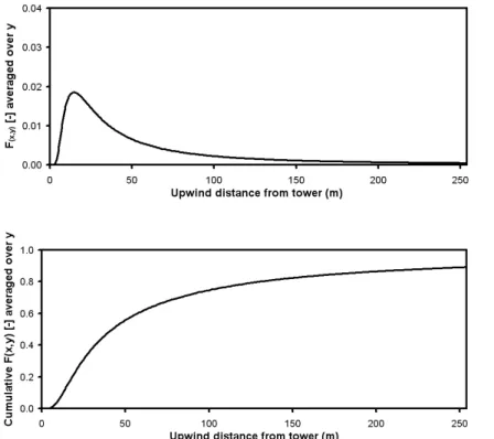
3.4 Footprint model

The location and extent of the footprint depends on surface roughness, atmospheric stability, wind speed, wind direction and may cover many pixels upwind of the eddy co-variance tower (Schmid and Oke, 1990; Hsieh et al., 2000). There are several types of footprint models. Initially, simple two-dimensional analytical footprint models for neutral

5

atmospheric conditions were developed (Gash, 1986; Schuepp et al., 1990). Later, the analytical footprint model was improved to account for atmospheric stability conditions (Horst and Weil, 1992; Hsieh et al., 2000). The footprint flux,F(x,z_s) [–], along the up-wind direction,x [m], measured at the heightzs [m], suggested by (Hsieh et al., 2000) is used in this study.

10

A typical footprint size and footprint intensity for one 30 min period on 19 Au-gust 2002, at a Rio Grande saltcedar EC tower is presented in Fig. 2. To verify the quality of the footprint model used in this study, we also calculated xmax (peak foot-print) for this period with the model by Schuepp et al. (1990). The models by Hsieh et al. (2000) and Schuepp et al. (2000) calculatexmax as 10 m (Fig. 2) and 11 m,

re-15

spectively, which implies that the footprint from Hsieh et al. (2000) is indeed close to the tower. At most EC sites, the maximum contribution to the footprint was within 50 m from the tower (wind speeds were generally less than 4 ms−1) and most of the footprint in-tensity (>90 %) is located within 300 m from the tower. We compute the footprints from meteorological parameters including air temperature, sensible heat flux, wind speed,

20

wind direction and friction velocity. The footprints for H and LE are obtained for the time of the satellite overpass using the 30 min averaged meteorological parameters. Approximately 80 % of all footprint fluxes cover an area of 5 to 9 pixels, twenty percent cover larger areas. As explained in Sect. 3.3.3 calculation of a representative daily footprint for comparison of SEBALH and LE estimates and ground measurements is

25

(18)

HESSD

11, 13479–13539, 2014

riparian areas

S.-H. Hong et al.

Title Page

Tables Figures

◭ ◮

Back Close

Full Screen / Esc

Discussion

P

a

per

|

Discussion

P

a

per

|

Discussion

P

a

per

|

Discussion

P

a

per

|

3.5 Calibration and evaluation of SEBAL flux predictions

This study cannot be a robust validation study due to missing soil heat flux measure-ments in the Middle Rio Grande Valley and biased net radiation measuremeasure-ments over heterogeneous riparian vegetation with patches of bare soil. Our aim is to evaluate the challenges of SEBAL flux predictions in arid riparian areas using a validation approach.

5

Calibration is the process of adjusting hydrologic model parameters to obtain a fit to observed data. In SEBAL the relationship between model parameter ∆T and re-motely observed radiometric surface temperatureTs in Eq. (4) is calibrated using the remotely observed energy balance components ofRnandGat two extreme conditions in a Landsat image: the cold wet pixel and hot dry pixel.

10

After calibration, validation tests typically are applied to a second set of data to test the performance of a hydrologic model. In the context of this study the second data set consists of ground measurements ofRn,G,H and LE, at pixels other than the cold and hot pixels. Validation or evaluation is accomplished by comparing the SEBAL predicted energy balance components with the ones measured on the ground at locations with

15

eddy covariance towers.

Calibration approaches

The temperatures of the cold and hot pixel for the derivation of calibration coefficients c1andc2in Eq. (4) are most critical in SEBAL as well as METRIC since they constrain LE between its maximum value at the cold wet pixel and zero at the hot dry pixel

20

by reducing biases inH associated with uncertainties in aerodynamic characteristics includingTs (Bastiaanssen et al., 2005; Allen et al., 2006). In SEBAL this calibration is entirely based on information that is available inside the image and, therefore, it is called “self-calibration” (Bastiaanssen et al., 2005) or “internalized calibration” and “autocalibration”.

25

Over the cold pixel it is assumed that ∆T =0, which implies that H=0 and LE=

(19)

HESSD

11, 13479–13539, 2014

riparian areas

S.-H. Hong et al.

Title Page

Tables Figures

◭ ◮

Back Close

Full Screen / Esc

Discussion

P

a

per

|

Discussion

P

a

per

|

Discussion

P

a

per

|

Discussion

P

a

per

|

observations for the calculation of the reference ET (Allen et al., 1998) for the estima-tion ofHin well-irrigated alfalfa and clipped grass fields (Allen et al., 2007, 2011). How-ever, this study deals with a SEBAL application in riparian areas without high quality hourly meteorological observations as is the default condition for many regions world-wide (Droogers and Allen, 2002). The selection of the hot pixel is quite challenging

5

because the heterogeneous landscapes of the southwestern US include quite a few hot and dry areas with a wide range of temperatures. In this study, the hot pixel is se-lected from a dry bare agricultural field where ET is just close to zero. Therefore, for any pixel cooler than the hot pixel, ET>0 (if theRnandGare the same), and for any pixel warmer than the hot pixel, for example a parking lots, ET=0. In addition, the equation

10

forG estimation was derived for agricultural conditions and therefore produces more dependable estimates for calibration when applied to a bare, agricultural soil having a tillage history.

As a consequence of the “internalized calibration” any biases inRn orG at the hot pixel in the image are transferred intoH. However, this bias introduced intoH is

trans-15

ferred back out of the energy balance during the calculation of LE from Eq. (1), since the bias is present in bothRn−GandH, and thus cancels (Allen et al., 2006). The “in-ternalized calibration” results in the least biased LE if the cold and hot pixel are properly selected and is the most distinctive feature of SEBAL and METRIC compared to other remote sensing LE algorithms.

20

The selection of cold and hot pixel requires a thorough understanding of field mi-crometeorology and is somewhat subjective, i.e. different experts will select slightly di_fferent temperature values. The cold pixel is selected where areas with well-watered healthy crops with full soil cover or in shallow water bodies (Allen et al., 2011; Basti-aanssen et al., 2005) and is relatively straightforward while the hot pixel selection is

25

(20)

HESSD

11, 13479–13539, 2014

riparian areas

S.-H. Hong et al.

Title Page

Tables Figures

◭ ◮

Back Close

Full Screen / Esc

Discussion

P

a

per

|

Discussion

P

a

per

|

Discussion

P

a

per

|

Discussion

P

a

per

|

et al., 2005; Kleissl et al., 2008) the value of ground measurements for calibration of SEBAL is not well established. For this reason we test two different calibration ap-proaches for the selection of the temperatures for the cold and hot pixel: the Empiri-cal(EM) approachand the Eddy Covariance (EC)approach. The former is based on inspection of the hydrogeological features of the landscape and qualitative

microme-5

teorological considerations and is typical for most SEBAL applications since the high number of EC towers available in this study is a unique situation. The Eddy Covariance (EC) approach is based on inspection of the hydrogeological features of the landscape followed by fine-tuning the parameters c1 (slope) and c2 (intercept) in Eq. (4) using ground measurements of instantaneous latent heat fluxes at the EC towers after

ad-10

justment for closure error. Since selection of the cold pixel is straightforward in fully vegetated fields, the temperature of the cold pixel was fixed but the temperature of the hot pixel was varied to best match the instantaneous ground measurements of LE (Hong, 2008). In order to independently evaluate the EM vs. the EC approach, senior author Hong implemented the EC approach, while co-author Hendrickx implemented

15

the EM approach.

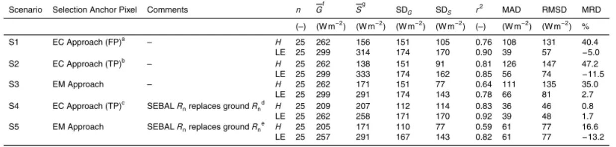
Five di_fferent calibration scenarios (S1–S5) were implemented and compared (Ta-ble 3). In the EC approach, calibration of SEBAL to ground measurements was im-plemented either using the average footprint weighted instantaneous SEBAL LE heat fluxes (S1, EC_FP) or using the instantaneous SEBAL LE heat flux of the pixel where

20

the EC tower is located (S2, EC_TP). The former method is difficult to implement for most practitioners while the latter is practical and fast but requires homogeneous con-ditions around the tower to the maximum extent of the footprint. The EM approach (S3) was implemented without using the LE’s measured by the EC towers or any other meteorological measurements.

25

(21)

HESSD

11, 13479–13539, 2014

riparian areas

S.-H. Hong et al.

Title Page

Tables Figures

◭ ◮

Back Close

Full Screen / Esc

Discussion

P

a

per

|

Discussion

P

a

per

|

Discussion

P

a

per

|

Discussion

P

a

per

|

impact of using the more accurate SR_nfor energy balance closure in the EC approach on the tower pixel (S4, EC_TP/SRn) and in the EM approach (S5, SRn).

4 Results and discussion

4.1 Spatio-temporal distribution of daily latent heat fluxes

Figure 3 presents an example of the ET maps produced by SEBAL. Similar maps for

5

the other components of the energy balance as well as other environmental parameters such as albedo, NDVI, surface temperature, etc. can be generated. In Fig. 3, daily ET rates are mapped in the Middle Rio Grande Valley and surrounding deserts on four different days during the spring, summer and fall. The maps show how the ET rates increase from 7 April (just after the start of the irrigation season) to 16 June at the

10

height of the irrigation season; a decrease of ET is observed during September and October when fields are harvested and lower temperatures are impeding crop growth. On all four days higher ET rates are observed over irrigated fields and in the riparian areas while low to very low rates occur in the surrounding deserts.

4.2 Comparison of SEBAL net radiation with ground measurements

15

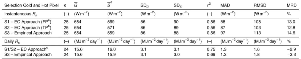
Figures 4 and 5 and Table 4 present the comparisons of the instantaneous and dailyRn measured on the ground and estimated by SEBAL. The MADs are 88/87 and 97 W m−2 for the EC approaches (S1/S2) and Empirical Approach (S3), respectively, resulting in MRDs of 13.0/12.8 and 14.6 %. These differences are about two to three times larger than those typically reported for SEBAL (Jacob et al., 2002; Allen et al., 2006). The

20

(22)

HESSD

11, 13479–13539, 2014

riparian areas

S.-H. Hong et al.

Title Page

Tables Figures

◭ ◮

Back Close

Full Screen / Esc

Discussion

P

a

per

|

Discussion

P

a

per

|

Discussion

P

a

per

|

Discussion

P

a

per

|

A bias occurs where the net radiometer is placed preferentially above vegetation that has a lower albedo, lower surface temperature and higher surface emissivity than the patches of bare soil next to the vegetation in the Landsat pixel. Increasing MRDs with increasing heterogeneity of the land surface have been observed in Arizona where the MRD’s between ground measured Rn’s and the one’s estimated with a remote

5

sensing algorithm were 1.2, 9.2, and 17.2 %, respectively, for a homogeneous cotton field, heterogeneous shrub terrain, and heterogeneous grassland (Su, 2002). The MRD of 9.2 and 17.2 % from the heterogeneous pixels are similar to the ones reported in Table 4.

Contrary to the instantaneous values, the daily net radiations measured on the

10

ground and determined in SEBAL match very well with MRDs of only−2.3 to−2.9 %. This immediately begs the question “why?” since the instantaneousRn’s differ by more than 12 %. On clear days over sparsely vegetated surfaces the maximum temperature di_fference between bare soil and vegetation typically occurs around noon. For example, temperature differences measured in the Walnut Gulch Experimental Watershed near

15

Tombstone, Arizona, varied between 10 and 25◦C during that time of the day (Humes et al., 1994). Since the conditions in the arid riparian areas of this study are similar, we expect similar temperature differences to occur when the satellite passes over around 10:30 a.m. The incoming short and longwave radiation are equal for the bare soil and the vegetation; therefore the net radiation will depend on the outgoing short and long

20

wave radiation. The albedo and surface temperature of dry bare soils during the day are higher than of vegetation resulting in more reflection of short wave radiation and more emission of long wave radiation which results in a lower Rn during the day for bare soil. During the night the surface temperatures of vegetation and bare soil are similar so that –due to the higher emissivity of vegetation (0.99) as compared to bare

25

(23)

HESSD

11, 13479–13539, 2014

riparian areas

S.-H. Hong et al.

Title Page

Tables Figures

◭ ◮

Back Close

Full Screen / Esc

Discussion

P

a

per

|

Discussion

P

a

per

|

Discussion

P

a

per

|

Discussion

P

a

per

|

These differences have been quantified by comparing the SEBAL estimated instan-taneous and daily net radiation for fully vegetated agricultural fields, saltcedar, and bare soils (Table 5). Whereas the measured instantaneous net radiation fluxes of fully cropped agricultural fields and saltcedar stands exceeded those of bare soils by 54 to 77 %, the daily net radiation fluxes were only 20 to 36 % larger. A typical Leaf

5

Area Index (LAI) for saltcedar in the Middle Rio Grande Valley is about 2.5 (Cleverly et al., 2002) which indicates that bare soil is present but vegetation cover is domi-nant. Now let us assume a typical mixed pixel with a soil cover of 75 % saltcedar and 25 % bare soil. The data from Table 5 for the first saltcedar plot show that the ra-tios between 100 % saltcedar and 100 % bare soil for, respectively, instantaneous and

10

daily net radiation are 1.77 and 1.34. We want to find similar ratios between 100 % saltcedar and our mixed pixel using the values of Table 5 for the instantaneous and daily net radiation for saltcedar and bare soil. Ignoring the effect of thermal radiation from soil that is intercepted by adjacent vegetation, the instantaneous and daily net radiations for the mixed pixel are, respectively, 0.75×670+0.25×379=598 W m−2

15

and 0.75×19.8+0.25×14.8=14.9+3.7=18.6 MJ m−2day−1. So, the net instanta-neous and daily radiations of a fully vegetated saltcedar pixel are 670/598=1.12 and 19.8/18.6=1.06 times those of our mixed pixel. The 12 % difference is similar to the MRD’s of 13–15 % presented for the difference in instantaneous net radiation between ground measurements and SEBAL estimates. The 6 % di_fference for daily net radiation

20

falls within error ranges of radiation measurements (Halldin and Lundroth, 1992; Field et al., 1992). Thus, the much smaller MRD for dailyRn(−2.3 to 2.9 %) compared to the MRD of instantaneousRn (about 13 %) can be explained by environmental radiation physics and is not caused by bias in the SEBAL method for determination of instan-taneous Rn or in the radiation sensors. This leads to the conclusion that the SEBAL

25

(24)

HESSD

11, 13479–13539, 2014

riparian areas

S.-H. Hong et al.

Title Page

Tables Figures

◭ ◮

Back Close

Full Screen / Esc

Discussion

P

a

per

|

Discussion

P

a

per

|

Discussion

P

a

per

|

Discussion

P

a

per

|

4.3 Comparison of SEBAL soil heat flux with ground measurements

The magnitude of soil heat fluxG depends on surface cover, soil water content, and solar irradiance. For a moist soil beneath a plant canopy or residue layer the instanta-neousG will often be less than±20 W m−2(Sauer, 2002b) while a bare, dry, exposed soil in midsummer could have a day-peak in excess of 300 W m−2(Fuchs and Hadas,

5

1973). In the Middle Rio Grande Basin during summer typical midday (10 a.m. through 2 p.m.) values of G are 104 and 132 W m−2 _{for, respectively, upland grassland and}

shrubs (Kurc and Small, 2004). These values demonstrate that the instantaneous G in riparian areas can be an important component of the instantaneous energy balance that needs to be taken into account. In most field soils the instantaneousGexhibits not

10

only a temporal variability but also a large spatial variability which makes it very difficult to measure an averageGfor areas with the size of a typical Landsat pixel (30 m×30 m) (Sauer, 2002b).

For this study six soil heat flux measurements were available from the Owens Valley and the San Pedro Valley. The SEBAL determinedGapproaches the ground measured

15

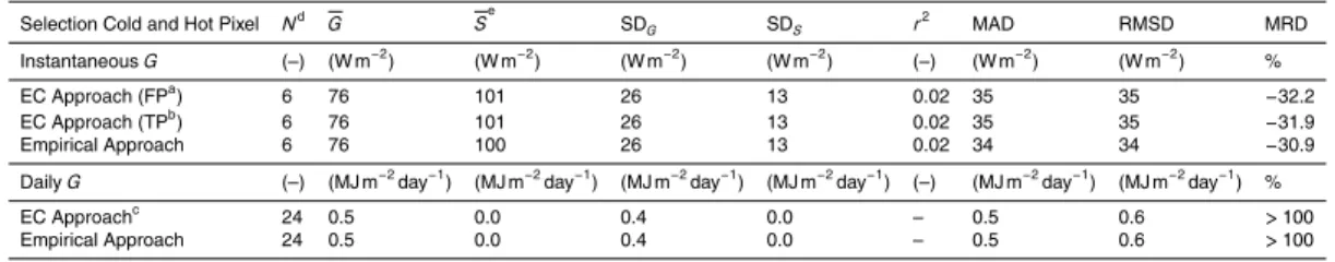
Greasonably well (Fig. 6) but the MRD is relatively high with values of 30.9 to 32.2 % (Table 6). However, the overall impact of the relatively high MRD in instantaneousGis minor since its MAD of 35 W m−2 (Table 6) hovers around 6 % percent of the SEBAL predicted instantaneous net radiation and around 5 % percent of the ground measured instantaneous net radiation. The daily G is close to zero since heat enters the soil

20

during the day but leaves the soil during the night. The dailyG measurements in the field confirm this (Table 6). Therefore, it is assumed in SEBAL that the daily heat flux can be neglected, i.e.Gis zero.

Given the high spatial and temporal variability ofG (Sauer, 2002b) within one Land-sat pixel, the reasonable agreement between SEBAL predicted instantaneousG and

25

(25)

HESSD

11, 13479–13539, 2014

riparian areas

S.-H. Hong et al.

Title Page

Tables Figures

◭ ◮

Back Close

Full Screen / Esc

Discussion

P

a

per

|

Discussion

P

a

per

|

Discussion

P

a

per

|

Discussion

P

a

per

|

0.001 m2, it appears that the SEBAL estimatedGresults in a quite acceptable estimate on the pixel scale.

4.4 Comparison of SEBAL sensible and latent heat fluxes with ground

measurements

Since there is a strong interplay between sensible and latent heat fluxes we discuss

5

both heat fluxes together in this section. First we inspect the plots of instantaneous and daily SEBAL heat flux estimates vs. ground measurements (Fig. 7) that demonstrate several interesting features. Our data set covers a wide range of conditions varying from dry to moist which allows evaluation of SEBAL over a wide range of environmen-tal conditions in riparian areas. The ground measured instantaneous and daily sensible

10

heat fluxes have, respectively, two and six negative data points which is an indication of the occurrence of regional advection. This advection is relatively minor for the instan-taneous fluxes during satellite overpass around 10:30 a.m. but increases considerably during late morning and early afternoon as reflected in the daily fluxes. The SEBAL estimated instantaneous and daily sensible heat fluxes that correspond to negative

15

values of the ground measurements are close to zero since the surface temperatures of their pixels are close to the cold pixel’s temperature. When high quality hourly me-teorological data are available regional advection can be accounted for in SEBAL by defining an advection enhancement parameter that is a function of soil moisture and weather conditions (Bastiaanssen et al., 2006; Allen et al., 2011) or one could

imple-20

ment METRIC (Allen et al., 2007). However, in this study our aim is to evaluate the performance of the traditional SEBAL in heterogeneous arid environments where no weather data are available. The data in Fig. 7 show that ignoring regional advection results in a maximum underestimation of the instantaneous and daily latent heat fluxes by, respectively, about 10 and 20 % under moist conditions; it becomes considerably

25

(26)

HESSD

11, 13479–13539, 2014

riparian areas

S.-H. Hong et al.

Title Page

Tables Figures

◭ ◮

Back Close

Full Screen / Esc

Discussion

P

a

per

|

Discussion

P

a

per

|

Discussion

P

a

per

|

Discussion

P

a

per

|

with our evaluation of the traditional SEBAL approach that does not take advection into account (Allen et al., 2011; Bastiaanssen et al., 1998a).

4.4.1 Comparison of instantaneous heat fluxes

Figures 8 and 9 present plots of, respectively, the adjusted sensible and latent heat fluxes measured at the EC towers vs. the SEBAL estimates resulting from scenarios

5

S1 through S5. While there exists a severe mismatch between the SEBAL estimated instantaneous sensible heat fluxes and the ground measurements (S1–S3), once the SEBAL estimated net radiation is used in the “ground measured” energy balance good agreement is reached (S4 and S5). SEBAL estimated instantaneous latent heat fluxes and ground measurements show good agreement for all five scenarios (S1–S5)

in-10

cluding the ones with a poor sensible heat flux match (S1–S3). Table 7 presents the quantitative comparison measures for these instantaneous fluxes. The prediction of latent heat fluxes is good for scenarios S1–S5 with a mean MRD of−5.1 % which is less than the average 14 % instantaneous deviation reported for SEBAL applications worldwide (Bastiaanssen et al., 2005).

15

The ground measured instantaneous H and LE are identical in S1–S3 but differ slightly from each other in S4 and S5 due to a slight difference in the temperature of the cold pixel that is also used for the estimation of the air temperature for calculation of the incoming long wave radiation. As a result the instantaneous net radiations of S4 and S5 are also slightly different. However, a large difference exists between the

20

ground measuredH and LE in S1–S3 vs. those in S4–S5. This is caused by the bias in instantaneous net radiation of the ground measurements vs. the net radiation de-termined with SEBAL (Table 4). In Table 7 theH and LE SEBAL estimates for the EM approaches (S3 and S5) are identical since this approach does not use the EC mea-sured instantaneous LE for calibration; one set of cold and hot pixels are used for both

25

(27)

HESSD

11, 13479–13539, 2014

riparian areas

S.-H. Hong et al.

Title Page

Tables Figures

◭ ◮

Back Close

Full Screen / Esc

Discussion

P

a

per

|

Discussion

P

a

per

|

Discussion

P

a

per

|

Discussion

P

a

per

|

instantaneous LE measurements at the EC towers. This leads to quite differentH and LE SEBAL estimates in S1, S2 and S4.

In scenarios S1 and S2 of Table 7 there is no significant difference between the SEBAL estimated sensible (156 vs. 138 W m−2) and latent (314 vs. 333 W m−2) heat fluxes. Thus, SEBAL calibrations based on the instantaneous latent heat flux of the

5

tower pixels (S2) or on the latent heat flux of the instantaneous foot prints during the satellite’s overpass (S1) yield similar results in this study except that the MAD and RMSD of S1 are lower: MAD/RMSD values for S1 and S2 are 39/57 and 56/74, re-spectively. This finding is relevant for practitioners who need to calibrate SEBAL on a routine basis and/or in nearly real-time: using only the tower pixels is much faster

10

and easier to implement automatically than determination of a footprint weighted aver-age. It also justifies the omission of foot print scenario S1 from further consideration in scenario S4. However, for posterior SEBAL analyses and research applications use of the footprint is still recommended since (1) it results in somewhat smaller comparison measures (Table 7) and (2) footprint analyses are effective for the detection of unusual

15

environmental conditions.

The MAD and RMSD of the sensible heat fluxes for S1, S2 and S3 are quite sim-ilar but rather high with MAD/RMSD values of, respectively, 108/131, 126/147 and 111/135. The values of S4 and S5 36/46 and 61/77 are considerably lower and reflect the ground energy balance correction by using the SEBAL net radiation. The

20

MAD/RMSD values of the latent heat fluxes are increasing from a low value of 39/57 for S1, 56/74 for S2 to 66/81 for S3 while the values for S4 and S5 are, respectively, 39/48 and 61/77. Thus, using the net radiation correction has a much smaller effect for the latent heat fluxes than for the sensible heat fluxes which is a result of the internal calibration of SEBAL. The comparison measures for S3 and S5 (the empirical

tradi-25

tional SEBAL approach) are also very similar for the latent heat flux but are reduced in half for the sensible heat flux after net radiation correction.

(28)

tem-HESSD

11, 13479–13539, 2014

riparian areas

S.-H. Hong et al.

Title Page

Tables Figures

◭ ◮

Back Close

Full Screen / Esc

Discussion

P

a

per

|

Discussion

P

a

per

|

Discussion

P

a

per

|

Discussion

P

a

per

|

perature as well as errors in narrow band emissivity, atmospheric correction, satellite sensor, aerodynamic resistance, and soil heat flux function. This can result in a re-duction of total bias in ET of as much as 30 % compared to other models that are not routinely internally calibrated (Allen et al., 2006). Allen et al. (2007) describe how MET-RIC, through the use of weather based reference ET, is able to eliminate most internal

5

energy balance component biases at both the cold and hot extreme conditions. SEBAL, on the other hand, eliminates biases at the hot extreme, but necessarily retains a bias at the cold extreme where it is assumed that LE=Rn−G. The cost for the improved estimates for LE is a deterioration of the SEBAL and METRICH estimates since the sensible heat flux, as an intermediate parameter, absorbs most of the aforementioned

10

biases as a result of the internal calibration process (Choi et al., 2009).

The same trends observed in the MAD and RMSD values are found in the MRD values presented in Table 7. A striking feature in S1–S3 is the very poor prediction of the sensible heat flux with MRD’s between 35 and 47 %. Especially, for S1 and S2 that have been calibrated against ground measured instantaneous latent heat fluxes, this

15

result was not expected. The discrepancy is not caused by any error in the SEBAL procedure but by the apparent bias in the ground measurements of the net radiation that was reported earlier (see Sect. 4.2). When the ground measured net radiation is replaced with the arguably more accurate SEBAL estimate of net radiation, the SEBAL estimates of sensible heat fluxes improve dramatically with MRD’s in S4 and S5 of,

20

respectively, 0.8 and 16.6 %. Despite the poor MRD’s ofH (35 to 47 %) in S1–S3 the SEBAL LE estimates exhibit good MRD’s (2.7 to−11.5 %). Therefore, these numbers provide an instructive demonstration of the power of SEBAL’s internal calibration.

We conclude that calibrating SEBAL with reliable ground measurements at the pixel scale will indeed improve its estimates of both, sensible and latent instantaneous heat

25