www.scielo.br/cam
Modeling and simulation of multi-component
aerosol dynamics
YALCHIN EFENDIEV
Department of Mathematics, Texas A&M University, College Station, TX 77843-3368 E-mail: [email protected]
Abstract. In this paper we consider the modeling of heterogeneous aerosol coagulation where the heterogeneous aerosol particles (called droplets) contain smaller particles (enclosures).
Droplets and enclosures coagulate with different collision kernels. We discuss macroscopic
mod-eling and simulation of these processes using both deterministic and Monte-Carlo methods.
Mathematical subject classification: 65C05, 65C35.
Key words:multi-component, aerosol, Monte Carlo, heterogeneous.
1 Introduction
The study of aerosol dynamics is often limited to homogeneous, single-component aerosol particles. Furthermore, even those studies that have em-ployed more than one component assume that aerosol is a homogeneous mixture of all multi-component constituents. However, it is known that phase segrega-tion will take place within an aerosol droplet if the thermodynamics and kinetics are favorable, in a manner analogous to that observed in bulk materials. So in order to accurately predict and control multi-component particle production it is not sufficient to assume that aerosol is a homogeneous mixture of all multi-component constituents. In a manner analogous to bulk materials our goal is to be able to control and characterize the overall behavior of the multi-component aerosol particles.
It is becoming increasingly apparent that multi-component aerosol particles are of both industrial importance and an area in need of significant research activity.
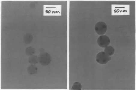
There have been a number of multi-component aerosol dynamics studies with het-erogeneous aerosol particles that have shown the importance of multi-component aerosol particles in material synthesis. There are experimental studies on the for-mation of binary metal oxide systems with application to removal of heavy metals [4, 5] as well as the formation of materials with novel and interesting properties [10, 11, 26]. One of the main goals in this research is to study the evolution of the internal state of the aerosol droplets and accurately predict and control their internal morphology. Initial success in growing interesting microstructures [26] indicated that further research was warranted. In subsequent studies both in-situ investigation into the formation process [18], multi-component aerosol dynamic modeling [3] and molecular dynamics computation [27] have been em-ployed. One of the primary conclusions was that for high temperatures where these materials are typically grown, nanodroplets are in liquid-like state, and that phase segregation taking place within the nanodroplet was probably limited by the transport within nanodroplet. This was one of our working assumptions in modeling and simulation [7, 8 9] of multi-component nanodroplets. In Figure 1 we present an example of TEM results for theSiO2/F e2O3system.
In the course of this paper, we shall use the terms minor phase and enclo-sure interchangeable to refer to the component within each aerosol droplet, and droplet or aerosol when referring to the major phase. The mathematical formu-lation of the problem allows one to consider the enclosures as particles inside the droplet that coagulate with collision kernel that is different from that of droplet coagulation. The temporal evolution of the aerosol and enclosures is schemat-ically depicted in Figure 2. Instantaneous coalescence assumption is used in the modeling that is justified by experiments. More detailed description of the experiment can be found in [26].
Figure 1 – Evolution of the aerosol (SiO2) and minor phase (F e2O3) during the growth
ofSiO2/F e2O3nanocomposites.
000 000 000 000 000 000 111 111 111 111 111 111 0000 0000 0000 0000 0000 1111 1111 1111 1111 1111 0000 0000 0000 0000 0000 0000 1111 1111 1111 1111 1111 1111 00000 00000 00000 00000 00000 00000 00000 11111 11111 11111 11111 11111 11111 11111 0000 0000 0000 0000 0000 0000 0000 1111 1111 1111 1111 1111 1111 1111 00 00 00 11 11 11 0000000 0000000 0000000 0000000 0000000 0000000 0000000 0000000 0000000 0000000 0000000 1111111 1111111 1111111 1111111 1111111 1111111 1111111 1111111 1111111 1111111 1111111 000 000 000 000 000 000 000 111 111 111 111 111 111 111 000000000000000 000000000000000 000000000000000 000000000000000 000000000000000 000000000000000 000000000000000 000000000000000 000000000000000 000000000000000 000000000000000 000000000000000 000000000000000 000000000000000 000000000000000 000000000000000 000000000000000 000000000000000 000000000000000 000000000000000 000000000000000 000000000000000 000000000000000 000000000000000 000000000000000 000000000000000 000000000000000 000000000000000 000000000000000 111111111111111 111111111111111 111111111111111 111111111111111 111111111111111 111111111111111 111111111111111 111111111111111 111111111111111 111111111111111 111111111111111 111111111111111 111111111111111 111111111111111 111111111111111 111111111111111 111111111111111 111111111111111 111111111111111 111111111111111 111111111111111 111111111111111 111111111111111 111111111111111 111111111111111 111111111111111 111111111111111 111111111111111 111111111111111 0000000 0000000 0000000 0000000 0000000 0000000 0000000 0000000 0000000 0000000 0000000 1111111 1111111 1111111 1111111 1111111 1111111 1111111 1111111 1111111 1111111 1111111 0000 0000 0000 0000 0000 0000 0000 0000 1111 1111 1111 1111 1111 1111 1111 1111 0000 0000 0000 0000 0000 0000 0000 1111 1111 1111 1111 1111 1111 1111 0000 0000 0000 0000 0000 0000 0000 1111 1111 1111 1111 1111 1111 1111 0000 0000 0000 0000 0000 1111 1111 1111 1111 1111 00000 00000 00000 00000 00000 00000 00000 00000 11111 11111 11111 11111 11111 11111 11111 11111 000000 000000 000000 000000 000000 000000 000000 000000 000000 111111 111111 111111 111111 111111 111111 111111 111111 111111 0000000 0000000 0000000 0000000 0000000 0000000 0000000 0000000 0000000 0000000 0000000 0000000 0000000 0000000 1111111 1111111 1111111 1111111 1111111 1111111 1111111 1111111 1111111 1111111 1111111 1111111 1111111 1111111 000000000 000000000 000000000 000000000 000000000 000000000 000000000 000000000 000000000 000000000 000000000 000000000 000000000 000000000 000000000 000000000 000000000 000000000 111111111 111111111 111111111 111111111 111111111 111111111 111111111 111111111 111111111 111111111 111111111 111111111 111111111 111111111 111111111 111111111 111111111 111111111 0000 0000 0000 0000 0000 0000 0000 0000 1111 1111 1111 1111 1111 1111 1111 1111 0000 0000 0000 0000 0000 0000 1111 1111 1111 1111 1111 1111 000 000 000 000 000 111 111 111 111 111 ENCLOSURES DROPLETS
Increasing Residence Time
Figure 2 – Schematic description of droplet-enclosure growth process.
macroscale models. Our argument is not mathematically rigorous and we back it up with physical arguments as well as with Monte-Carlo simulations. The global existence result for the generalized model that describes heterogeneous aerosol coagulation is also presented.
On the other hand, Monte Carlo methods have the advantage that multi-scale and time phenomena can be simultaneously solved without the requirement of a single unifying governing multi-variate equation. We discuss the difficulties of Monte-Carlo methods for heterogeneous aerosol coagulation processes due to the multiscale nature of these processes and the approaches to overcome these difficulties.
The paper is organized as follows. In the next section we discuss the determin-istic models and the assumptions involved in this modeling. Section 3 is devoted to numerical results. The conclusions are drawn in section 4.
2 Heterogeneous aerosol coagulation
2.1 Deterministic modeling of heterogeneous aerosol coagulation
Conceptually, there are two kinds of mathematical models describing the dynam-ics ofhomogeneousaerosol particles: deterministic and stochastic models. The deterministic models describe the evolution of some average quantities, e.g., the number density of aerosol particles with certain properties. For spherical parti-cles, we are usually interested in the number density of the partiparti-cles,N (t, V ), with volumeV. More precisely,N (t, V )dV is the number of aerosol particles with volumes betweenV andV+dV. The coagulation process is characterized by a collision kernel which describes the collision mechanism. The expression for the collision kernel is based on a physical model and particle properties (size, density, etc). The equation for the evolution ofN (t, V )was first introduced by Smoluchowski [23] (survey paper [6]):
dN (t, V )
dt =
1 2
V
0
K(U, V −U )N (t, U )N (t, V −U )dU
− N (t, V )
∞
0
K(V , U )N (t, U )dU.
(1)
The first term on the right hand side accounts for the gain of particles of volume
fragmentation, condensation, nucleation, diffusion and etc. Some of commonly used collisions kernels in aerosol coagulation ([12]) are free-molecule collision kernel
KF(U, V )=K0
1
U +
1
V
1/2
(U1/3+V1/3)2, (2)
where K0 =
3
4π
1/6
6kT ρ
1/2
and Brownian (continuum regime) collision
kernel
KD(u, v)=K0(u1/3+v1/3)
1
u1/3 +
1
v1/3
, (3)
whereK0=
2kT
3µ . Herekdenotes Boltzmann’s constant,T is the temperature, µis the viscosity of the medium comprising aerosol particles andρis the density of droplets. Throughout the paper we will assume that the collision kernels are homogeneous, i.e.,K(λu, λv)=λpK(u, v). Note that for free-molecule regime p=1/6 and for Brownian coagulationp=0.
For the heterogeneous aerosol coagulation we assume that the collision kernels for the enclosure coagulation (or coagulation of the minor phase) hasp = pe
and the collision kernel for the droplet coagulation hasp=pd. In particular, we are interested when the collision kernels for enclosure and droplet populations have different degrees of homogeneities (p). For iron/silica oxide binary system (see [7]), the collision kernel for enclosure coagulation haspe = 0, while the collision kernel for droplet population haspd=1/6.
The difficulty in mathematical modeling of the enclosure distribution of the whole system lies in the nonlinear nature of enclosure as well as in droplet coagulations. Assume that the collision kernel of the enclosures in each droplet is the same, and all droplets contain large number of enclosures so that we can describe their evolution by Smoluchowski’s equation. Denoting the number density of the enclosures in a droplet with volumeV, by nV(t, u)/V, we can write a population balance equation for the enclosures in a droplet of volumeV,
dnV(t, v)
dt =
1 2V
v
0
K(u, v−u)nV(t, u)nV(t, v−u)du
− 1
VnV(t, v)
∞
0
K(v, u)nV(t, u)du.
Note thatnV(t, u)duis the number of enclosures with volume betweenuand
u+duthat are in the droplet of volumeV. In general, in order to find the enclosure distribution for the whole system one needs to add the enclosure distributions over all droplets,
nt ot al(t, u)=
∞
0
nV(t, u)N (t, V )dV . (5)
Here we denote bynt ot al(t, u), the enclosure distribution of the whole system,
andN (t, V ) is the number density of the droplets. Since the equation (4) is nonlinear and the operation (5) is linear one cannot derive an equation for the evolution ofnt ot al(t, u) analytically. Moreover, it is not possible to describe
the individual enclosures inside individual droplets since the numerical efforts would be tremendous.
One of approaches in modeling is to limit the description of enclosure popu-lation to their basic statistics. This idea is utilized for a simple two-component system characterizingSiO2/F e2O3, in one of our work [7]. A goal is to model Nn,u,σ(t, V ), which is the number density of aerosols with volumeV andn en-closures whose size distribution is characterized only by their (enen-closures) mean volumeuand standard deviationσ. Note that here we assume that the enclo-sure population has log-normal distribution. This assumption will be discussed in details below. The equation for the evolution ofNn,u,σ(t, V )can be written based on conservation principles (see [7])
dNn,u,σ(t, V )
dt =
1 2
V
0
K(U, V −U )
Nk′
,u′,σ′(t, U )Nk′′,u′′,σ′′(t, V −U )dU
−Nn,u,σ(t, V )
∞
0
K(U, V )Nk′
,u′,σ′(t, U )dU
+γ(k′
,u′,σ′)→(n,u,σ )(t, V )Nk′,u′,σ′(t, V )
−γ(n,u,σ )→(k′
,u′,σ′)(t, V )Nn,u,σ(t, V ).
(6)
cumbersome (the details in [7]). For example, in the first term the summation is taken over all possible(k′, u′, σ′)and(k′′, u′′, σ′′)such that if two droplets with volumeU andV −U and enclosure distribution characterized by(k′, u′, σ′)
and(k′′, u′′, σ′′)collide then the enclosure distribution of the resulting droplet is characterized by(k, u, σ ). The last two terms refer to the gain and loss due to interaction of the enclosures inside a droplet of volumeV. The quantity
γ(k′
,u′,σ′)→(n,u,σ )(t, V )denotes the rate that in a droplet of volumeV the
distri-bution of enclosure population will change from(k′, u′, σ′)to(n, u, σ )during the timedt. The details of the summation are again omitted.
In order to findγ(k′
,u′,σ′)→(n,u,σ )(t, V )we need to model the evolution of
ba-sic statistics of the enclosure population in each droplet. The latter can be easily done by multiplying Smoluchowski’s equation byvi (i = 0,1,2) and
integrating over all v ([7, 16]). This yields the following equations for the momentsdM0/dt = −K[M02+M1/3M−1/3], dM1/dt = 0, anddM2/dt =
2K[M12+M4/3M2/3], whereMi =
vin(v, t ). To close this system an assump-tion about the nature of the enclosure distribuassump-tion is needed. It is known that for large times the enclosure distribution can be approximated by the log-normal distribution [16, 20, 19]. Assuming that the enclosure distribution is log-normal
Mk = nvk gexp
9 2k
2log2(σ )
one can derive an evolution equation forn(the
total number of particles),vg(the geometric mean particle volume), andσ (the geometric standard deviation), from where γ (see eq. (6)) can be computed analytically (see [7]). To solve (6) we employed binning strategy that divides the space of droplet volumes and enclosure numbers into coarse partitions [7]. The latter is necessary because the range of droplet volumes and the number of enclosures is very large which makes it difficult to use standard discretization techniques.
2.2 Assumptions involved in deterministic modeling
of enclosure population in the resulting droplet is equal to the sum of the distri-butions of enclosure populations in the colliding droplets. Thus, it will remain log-normal if and only if the mean volume of the enclosures and their variance in the colliding droplets are the same.We claim that the mean enclosure volume of each droplet is the same among the droplets for large times providedpe < pd.
The mean enclosure volume of each dropletiis defined asui =Ui/ni, where
Uiis total enclosure volume in a dropleti, andniis the number of the enclosures in the dropleti. This fact (the equality of mean enclosure volumes) plays an important role in modeling of aerosol systems where the enclosure population is characterized only with its basic statistics (e.g., total number, mean and vari-ance). Furthermore, this assumption greatly reduces the number of unknowns of the problem and can be used for various simple models. To show the validity of this assumption we will need to discuss the following two facts (1) the equality of the enclosure concentration in each droplet for large times (2) the behavior of the mean enclosure numbers in each droplet. With these two results we can argue that the mean enclosure volume of each droplet is the same among the droplets for large times provided the mean number of enclosures increases. Note that the latter is true ifpe < pd.
The equality of the enclosure concentration in each droplet at large times.
Define the concentration of enclosures in a dropletibyci, which is given as the total enclosure volume in this droplet divided by the droplet volume. We assert thatciis independent ofi,ci =c. This assumption is true if initially the concen-tration of the enclosures in each droplet is uniform. Then these concenconcen-trations will remain constant. Indeed, if two droplets with volumesV1 andV2 collide,
then the total concentration of enclosures in a resulting droplet with volume
V1+V2will bec(V1+V2), i.e., concentration will remain constant equal toc.
with volumeV1andV2, and enclosure concentrationsc1andc2collide, then the
volume of the resulting droplet isV =V1+V2, and the enclosure concentration
isc=(c1V1+c2V2)/V. Thus the evolution ofN (t, V , c)is simply governed by dN (t, V , c)
dt =
1 2
V
0
K(U, V −U )
c
0
N (t, U, c1)N
t, U,cV −c1U V −U
dU dc1
−N (t, V )
∞
0
∞
0
K(V , U )N (t, U, c1)dU dc1.
(7)
Here the first term accounts for the gain of particles with volume V and the enclosure concentrationc. These particles are formed as a result of a collision of droplets with volumeU andV −U and enclosure concentrations c1 and
(cV −c1U )/(V −U ). Similarly, the second term accounts for the loss of
droplets with volume V and the enclosure concentration c. The asymptotics of these kinds of equations have been studied in [13, 21]. It was shown that
∞
0
∞
0 (c−c)V N (t, V , c)dV dcconverges to zero ast → ∞. We see from (7)
that the study of the concentration of enclosure population does not depend on the distribution of enclosure population in each droplet. This is a fundamental difference between this study and the study of mean number of enclosures per droplet as well as the study of mean enclosure volume of each droplet.
The behavior of the mean enclosure numbers in each droplet. The assump-tion of the equality of mean volume of enclosures in each droplet,ui, holds if
pe< pd, and it is approximate ifpe ≈pd. We do not have rigorous mathemat-ical proof of this fact, and will use physmathemat-ical argument as well as Monte-Carlo simulations to demonstrate this. For this reason, we introduce the mean num-ber of enclosures per droplet, i.e.,nt ot/Mt ot, wherent ot is the total number of enclosures, andMt ot is the total number of droplets. If we assumepe < pd it can be shown that the mean number of enclosures per droplet increases. Indeed, using the self-similar theories (see [1]) it can be shown that in each droplet the number of enclosures decays ast−1/(1−pe). This rate is the same for all the
en-closures, consequently the total number of enclosures decays ast−1/(1−pe). On
mean number of enclosures per droplet grows as t−1/(1−pe)+1/(1−pd). Thus if
pe < pd the mean number of enclosures in each droplet will increase as tγ,
γ = −1/(1−pe)+1/(1−pd) >0. We will confirm this rate in our Monte-Carlo computations.
Next we present our argument onui. The characteristic interaction (i.e., co-agulation) time for the enclosures in each dropletVi, is given by
tic =K0e Vi
ni , (8)
whereni are the number of enclosures in a dropleti andK0e is a constant that depends on the physical parameters (the background media). We assume that at an asymptotic condition, the characteristic interaction times for the enclosures in each droplet are balanced with the characteristic coagulation time for the droplets. Consequently, the characteristic interaction time for the enclosures is the same. Since the total enclosure volume of a droplet with volumeVi, iscVi,
ticcan be written as
tic =K0eui c ,
constant (independent of the droplet) for large times if the mean enclosure volume of each droplet is constant. Consider,S2 = (vi −v)2n(vi, t ) = M2−v2n,
whereM2=
vi2n(vi, t )dv,n(vi, t )is the number of enclosure with volumevi,
nis the total number of enclosures, andvis the mean enclosure volume. For two colliding droplets with enclosure distributionn′(v, t )andn′′(v, t )we haveM
2= M2′+M2′′. From where assuming thatv′ =v′′we haveS2=S
′
2+S
′′
2,n=n
′+n′′
. Then for standard deviations = S2/nwe haves = (n′S2′ +n
′′
S2′′)/(n′+n′′
). From here using argument similar to the analysis of the enclosure concentration we can show thatstends to a constant for large times. The rigorous proof of this fact is a subject of future study.
3 Numerical methods and results 3.1 Monte-Carlo methods
Monte Carlo methods to simulate particulate growth processes are not new, and the theoretical foundations have been discussed extensively in the literature [14, 24, 25]. Basically the Monte Carlo approach utilizes probabilistic tools to study a finite dimensional subsystem in order to infer the properties of the whole system. Here we briefly discuss Monte-Carlo methods used in our simulations. There are in general two types of finite-volume Monte-Carlo techniques. In the first approach, the user sets the time intervalt, and uses Monte-Carlo to decide which and how many events will be realized. This method is sometimes referred to as time driven Monte-Carlo. In the second approach, the user selects a single event and then advances the time by an appropriate increment. In the method presented here we employ the first method for the enclosures or minor phase, and the second method to describe the droplets/aerosol. More precisely, we first select a single coagulation event for the droplets, and compute the time
T required for this event. Then for each droplet we calculate the enclosure interactions occurred during this time interval.
At each step of the simulation, dropletsiwith volume Vi andj with volume
with initial number concentrationC0and total numberN0droplets in the
simu-lation. Then as outlined by Smith and Matsoukas [22] the effective real volume being simulated isN0/C0, so that one coagulation event in our (model) system
representsC0/N0actual droplets per unit volume. To connect our simulations
to real time we calculate the inter-event time, by noting that the time between two events is inversely proportional to the sum of the rates of all possible events. If for examplek successful events are realized, then the remaining number of droplets in the system isNk =N−k, and the total number concentration of the
systemCkis given byCk
C0 = Nk
N0
. The mean inter-event time afterkcoagulations
as [22]
Tk = 2N0
C0 Nk−1
i=1
Nk−1
j=1 KijF
. (9)
For each droplet we use the inter-event time to determine the number of suc-cessful enclosure interactions (coagulation driven growth) before the next droplet coagulation. This unfortunately restricts the time step, because modeling the in-ternal state of the droplets requires complete knowledge of enclosure distribution within each droplet.
In an analogous manner to that of the droplets we also define the mean inter-event time for the enclosures in a droplet of volumeV as
t = n−12V i=1
n−1
j=1KijD ,
wherenis the number of the enclosures, andn/V is their number density. The number of successful enclosure interactions inside the droplet during the time intervalT1is given by the integerkwhich satisfies
k
i=1
2V
KijD(n−i)(n−i−1) ≤T1
≤ k+1
i=1
2V
KijD(n−i)(n−i−1).
(10)
On the left hand side of (10) we have the total time needed for the coagulation of
When the number of droplets drops to half the initial value, we replicate the droplets and their internal state. In order to preserve the physical connection to real time, the topping up process must preserve the average behavior of the system corresponding to the time prior to topping up. In particular, one has to ensure that the characteristic time for droplet collisions stays the same, and to do this requires an increase in the system volume in proportion to the increase in droplets. On the other hand, if the number of enclosures in a droplet becomes too large for the simulation, one can truncate the enclosure system within a droplet by randomly picking a certain number of enclosures and adjusting the corresponding computational volume. A flow chart of our Monte Carlo algorithm is depicted in Figure 3.
For each droplet
Randomly choose two droplets and calculate their collision probability
Calculate the elapsed time, dT, for this coagulation event
Perform k enclosure interactions such that the total sum of inter−event times spent during the enclosure interactions greater than or equal to dT
Calculate the extra time spent during the enclosure interactions in each droplet. This quantity will taken into account during the next droplet coagulation event
Implement the coagulation of the chosen droplets and calculate the enclosure distribution for the new droplet
If the number of droplets is less than M/2 (M is the number of initial droplets),.
Increase the size of the computational domain twice. duplicate the particles with their internal state.
t=t+dT
Figure 3 – Flow chart of Monte Carlo algorithm.
3.2 Numerical results
In the numerical examples we will use different constants K0 for enclosure
coagulation, Ke
0 and for droplet coagulation K0d (see e.g. (3)). In the first
pe = 0, while droplets coagulate with constant collision kernelpd = 0, and takeK0e = 4.8e −18, K0d = 3.6e −9, φ = 5.2e −7, where φ is the total
concentration of the droplets (see [9]). In this case our assumption on the mean volume of the enclosures will not be exact as the number of the enclosures per droplet does not increase. In the Figure 4 we plot mean number of enclosures per droplet using our Monte-Carlo simulations. As we see from this figure that mean number of enclosures per droplet reaches constant as it was predicted sinceγ = 0. The experiments are performed for three different values ofM
(initial number of droplets) andm(initial number of enclosures in each droplet). Because the mean number of enclosures per droplet does not increase we do not expect our assumption onui(mean enclosure volume of each droplet) discussed in the previous section to hold. Hereui,i =1, . . . , Mdenote the mean enclosure volume in theith droplet, andMis the total number of droplets. To measure the variability ofui we introduce the normalized varianceu2
m/u 2
m, where
u2 m =
1
imi
i
miu2i, um= 1 imi
i miui,
mi is the number of the mean enclosure volumes with volumeui. Note that the normalized variance is 1 if alluiare equal, i.e., for uniformui. In Figure 5 we plot the normalized variance of mean enclosure volumes of each droplet,u1, . . . , uM
in the dropletiis given by cVi, whereVi are the volumes of the droplets. The coagulation of the droplets is independent of the enclosures and it is known that the normalized variance of the droplet volumes is almost 2, [12].
0 0.005 0.01 0.015 0.02 0.025 0.03 0
400 800 1200 1600 2000
time, seconds
mean number of enclosures per droplet
(500,4000) (1000,3000) (1500,1500)
Figure 4 – Mean number of the enclosures per droplet
t he t ot al number of t he enclosures t ot al number of droplet s
for three values of(M, m), whereMrefers to the initial number of the droplets andm refers to the initial number of the enclosures per droplet in our simulation. All droplets
and enclosures are initially monodisperse.ndesignates mean number of enclosures per droplet. Casepe=pd.
Our next set of numerical results describe the situation where the enclosures coagulate in the Brownian regime (3)pd = 0, while droplets coagulate in the free-molecular regime (2),pe =1/6. We consider growth at two temperatures 2300 K and 2600 K, both of which were operating conditions for experiments. The viscosity of the droplets will govern the rate of Brownian transport of the minor phase and therefore the growth rate of enclosures. The viscosity of the major component silica (SiO2) as a function of temperature is given by [15] µ=10−8.6625(1−3556.03K/T )(kg)/(m s). and the density ofSiO2is held constant
atρ =5.5g/cm3. With these constantsKe
0andK0d can be easily determined.
0 0.01 0.02 0.03 0.04 0.05 0.06 0.07 0.08 0.09 0.1 1
1.2 1.4 1.6 1.8 2 2.2
time,seconds
normalized variance
n ≈ 390
n ≈ 10.5
n ≈ 1.5
Figure 5 – The normalized variance (u2
m/u2m) of the mean enclosure volumes of each droplet for different mean number of enclosures per droplet. Casepe =pd.
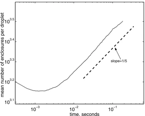
this rate in Figure 7 we plot the mean number of enclosures per droplet in a log-log scale along with a straight line with a slope 1/5. It is clear from this Figure that the growth of the mean number of enclosures per droplet has a rate 1/5. Since mean number of enclosures per droplet increases we expect that the mean enclosure volumes of each droplet will become uniform across droplet populations, i.e.,u1= · · · =uM, whereui is the mean enclosure volume ofith
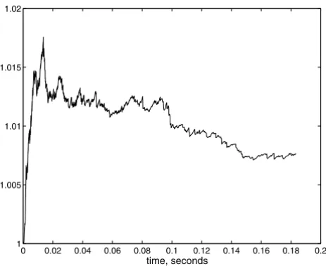
droplet andM is the number of the droplets. Indeed, Figure 8 shows this. In this Figure we plot the normalized variance of mean enclosure volumes of each droplet. Clearly, this number is close to one for large times (compare with the casepe =pd, Figure 5). We note that the constantsKe
0 andK0d(which depend
on physical parameters) do not affect growth rate.
0 0.02 0.04 0.06 0.08 0.1 0.12 0.14 0.16 0.18 0.2 1500
2000 2500 3000 3500 4000
time, seconds
mean number of enclosures per droplet
(1000,2000) (1500,1500)
Figure 6 – Mean number of the enclosures per droplet
t he t ot al number of t he enclosures t ot al number of droplet s
for two values of(M, m), whereMrefers to the initial number of the droplets andm
refers to the initial number of the enclosures per droplet in our simulation. All droplets and enclosures are initially monodisperse. Casepe=0,pd =1/6.
10−3 10−2 10−1
103.1 103.2 103.3 103.4 103.5
time, seconds
mean number of enclosures per droplet
slope=1/5
Figure 7 – Relative growth rate for differentk.α=1. The asymptote curve (designated
0 0.02 0.04 0.06 0.08 0.1 0.12 0.14 0.16 0.18 0.2 1
1.005 1.01 1.015 1.02
time, seconds
Figure 8 – The normalized variance
u2 m/u2m
of the mean enclosure volumes of each
droplet. Casepe=0,pd =1/6.
0 0.02 0.04 0.06 0.08 0.1 0.12 0.14 0.16 0.18 0.2 1000
1500 2000 2500 3000 3500 4000 4500
time, seconds
mean number of enclosures per droplet
(1000, 2000) sectional model
Figure 9 – Mean number of the enclosures per droplet
t he t ot al number of t he enclosures t ot al number of droplet s
One of the difficulties in Monte-Carlo simulations is the handling of the large number of enclosures within the droplets. Since we need to keep the number of droplets at some reasonable level, the increase in the number of enclosures per droplet makes our computations very difficult. Currently we are working on the approaches where the enclosure population in each droplet is carried only with three main statistics, the number of enclosure, the mean volume, and the variance. Each time when the detail enclosure population is needed we generate it from the log-normal distribution. If two droplets collide then the enclosure population is generated and a new droplet with whole new enclosure population is created. We carry full (detail) enclosure population for this droplet for some time until it relaxes to log-normal distribution. Then the enclosure population can be characterized with three moments. Our initial results look promising and the further research into the mathematical and computational aspects of this kind methods will be carried out.
4 Concluding remarks
In this paper we study the coagulation of heterogeneous aerosol particles and discuss main assumptions involved in deterministic modeling. In particular, we show that the mean volume of the enclosures per droplet is uniform for large times. The latter is crucial for the understanding of the heterogeneous coag-ulation processes. Because of multi-scale nature of the heterogeneous aerosol coagulation processes some innovative numerical methods are needed. We dis-cuss our current research on this direction.
A Global existence result for generalized Smoluchowski’s equation
We will consider a discrete coagulation model corresponding to the generalized Smoluchowski’s equation
dxj m
dt =
1 2
p+q=j,s+r=m
Kpqxpsxqr−
∞
p=1,r=1
Kjpxj mxpr+
∞
s=m Ams
j xj s. (11)
Herexij is the number of droplets whose volumei and containsj enclosures. We assume thatxj m(0)=cj m, such that
α < 1, and Aij ≤ C. Finite dimensional version of the equation (11) can be obtained through truncation up toN terms. The kernel is replaced byKij(N )as
Kij(N ) = Kij, ifi+j ≤N; 0 otherwise,
A(N )ij = Aij, ifi ≤N, j ≤N; 0 otherwise.
The finite dimensional version of (11) is
dxj m(N )
dt =
1 2
p+q=j,s+r=m
Kpq(N )xps(N )xqr(N )
− N
p=1,r=1
Kjp(N )xj m(N )xpr(N )+ N
s=m A(N )
ms j x
(N ) j s .
(12)
Next we introduce
Me =
j,m
xj m, Mv =
j,m
j xj m, Me(N ) = j,m
xj m(N ), Mv(N ) = j,m
j xj m(N ).
Lemma A.1. xj m(N )exist, unique andxj mN are positive.
Since the r.h.s. of (12) satisfies Lipschitz condition the solution exists, unique and bounded. Positiveness of the solution can be obtained similar to [17, 24].
The following can be checked directly
Lemma A.2.
dM(N ) v dt ≤0,
dM(N ) e
dt ≤0.
Then we have
xj m(N ) ≤
l,p
lxlp(N )=Mv(N )(t ) < C,|dxj m(N )/dt|
≤ 1
2
p,q,s,r
(p+q)xps(N )xqr(N )+
N
p,r
(j+p)xj m(N )xpr(N )+
N
s=m
A(N )ms
j x
(N ) j s
≤ C
p,s
pxps(N )
q,r
qxqr(N )+
j,s
xj s≤C.
From here using Ascoli’s lemma we obtain thatxj m(N ) converges along a subse-quenceNk uniformly in any time interval. Denotexj m =limN→∞x
(N ) j m for the
subsequence. Note thatxj mhas bounded first moments becausexj m(N )has bounded first moments independent ofN. To show thatxj m satisfies equation (11) we need to show that
p
Kjp(N )xpm(N ) → p
Kjpxpm, N → ∞
p
A(N )ms xj s(N )→ p
Amsxj s N → ∞.
(14)
Consider
p
Kjpxpm−
p
Kjp(N )xpm(N )
≤ p<N1
|Kjpxpm−Kjp(N )xpm(N )|
+ p>N1
Kjpxpm+
p>N1
Kjp(N )xpm(N ).
(15)
The first term can be made small by choosing N large enough, the second (and third term) can be made small by choosingN1large enough in the
follow-ing way:
p>N1
Kjpxpm ≤
p>N1
jαxpm+ p>N1
pαxpm
≤ jαN1−1 p>N1
pxpm+N1α−1 p>N1
pxpm
≤jαN1−1Mv(t )+N1α−1Mv(t )→0, ∀j, m.
(16)
Furthermore,
s
Amsxj s− s
A(N )ms xj s(N )
≤ s<N1
|Amsxj s−A(N )ms xj s(N )|
+ s>N1
Amsxj s+ p>N1
A(N )ms xj s(N )
ChoosingN large we make the first term small. ChoosingN1 large such that N1≫mwe can make the second and third terms small.
Uniqueness of the solution can be obtained in a manner analogous to [2].
REFERENCES
[1] D.J. Aldous,Deterministic and stochastic models for coalescence (aggregation and coagula-tion): a review of the mean-field theory for probabilists, Bernoulli,5(1999), 3–48.
[2] J.M. Ball and J. Carr,The discrete coagulation-fragmentation equations: existence, unique-ness, and density conservation, J. Statist. Phys.,61(1990), 203–234.
[3] P. Biswas, C.Wu, M.R. Zachariah and B.K. McMillen,Vapor phase growth of iron oxide-silica nanocomposite; Part II: Comparison of a discrete-sectional model predictions to experimen-tal data, J. Mat. Res, (1997), 714.
[4] P. Biswas, G. Yang and M.R. Zachariah,In situ processing of ferroelectric materials from lead streams by injection of gas-phase titanium precursors, Combustion Science and Technology, (1998), 183.
[5] P. Biswas and M.R. Zachariah,In situ immobilization of lead species in combustion environ-ments by injection of gas phase silica sorbent precursors, Env. Sci. Tech., (1997), 2455.
[6] R. Drake,A general survey of teh coagulation equation. in g.m. hidy and j.r. brock, editors, Topics in current aerosol research, (1972), 201–376.
[7] Y. Efendiev, M. Luskin, H. Struchtrup and M.R. Zachariah,A hybrid sectional-moment model for coagulation and phase segregation in binary liquid nanodroplets, J. Nanoparticle Res.,
4(2002), 61–72.
[8]Y. Efendiev and M.R. Zachariah,Hybrid monte-carlo method for simulation of two-component aerosol coagulation and phase segregation, J. Colloid Inter. Sci.,49(1) (2001), 30–43.
[9] Y. Efendiev and M.R. Zachariah,A model for two-component aerosol coagulation and phase separation: A method for changing the growth rate of nanoparticles, Chem. Eng. Sci,
56(2001), 5763.
[10] S. Ehrman, M. Aquino-Class, and M.R. Zachariah, Effect of temperature and vapor-phase encapsulation on particle growth and morphology, J. Materials Research, (1999), 1664–1671.
[11] S. Ehrman, S.K. Friedlander and M.R. Zachariah,Characterization ofSiO2/T iO2 nanocom-posite aerosol in a premixed flame, J. Aerosol Science, (1998), 687.
[12] S.K. Friedlander,Smoke, Dust and Haze, Oxford, (2000).
[14] D. Gillespie,An exact method for numerically simulating the stochastic coalescence process in cloud, J. Atmos. Sci., (1975).
[15] G. Jans, F.D.G. Lakshminarayanan, P. Lorentz and R. Tomkins,Molten Salts: Volume 1, Electrical Conductance, Density, and Viscosity Data, U.S. National Standard Reference Data Series, U.S. National Bureau of Standards, Washington, (1968).
[16] K.W. Lee,Change of particle size distribution during Brownian coagulation, J. Coll. Inter. Sci., (1983), 315–325.
[17] J.B. McLeod,On an infinite set of nonlinear differential equations, Quart. J. Math. Oxford Ser.,13(1962), 119–128.
[18] B.K. McMillin, P. Biswas and M.R. Zachariah,In situ characterization of vapor phase growth of iron oxide-silica nanocomposite: Part I: 2-d planar laser-induced fluorescence and mie imaging.J. Mat. Res., (1996), 1552–156.
[19] E. Otto, F. Fissan, S. Park and K. Lee,Brownian coagulation in the transition regime using the moments of a lognormal distribution, J. Aerosol Sci., (1997), 629–630.
[20] E. Otto, E. Stratmann, F. Fissan, H. Vemury and S. Pratsinis,Brownian coagulation in the transition regime. 2: a comparison of two modeling approaches, J. Aerosol Sci., (1993), 535–536.
[21] V. Piskunov and A. Golubev,Method for defining dynamical parameters of coagulating systems (in russian), Doklady Akademii Nauk,366(3) (1999), 341–344.
[22] M. Smith and T. Matsoukas,Constant-number Monte Carlo simulation of population bal-ances, Chemical Eng. Science, (1998), 1777–1786.
[23] M. Smoluchowski,Drei vorträge über diffusion, brownsche bewegung und koagulation von kolloidteilchen, Physik. Z., (1916), 557–585.
[24] J. Spouge,Monte-Carlo results for random coagulation, J. Colloid Interface Sci., (1985), 38.
[25] P. Tandon and D. Rosner,Monte Carlo simulation of particle aggregation and simultaneous restructuring, J. Colloid Interface Sci, (1999), 273–276.
[26] M.R. Zachariah, M. Aquino-Class, R. Shull and E. Steel,Formation of superparamagnetic nanocomposite from vapor phase condensation in a flame, Nanostructured Materials, (1995), 383.