www.geosci-model-dev.net/7/1691/2014/ doi:10.5194/gmd-7-1691-2014
© Author(s) 2014. CC Attribution 3.0 License.
Development of the Surface Urban Energy and Water Balance
Scheme (SUEWS) for cold climate cities
L. Järvi1, C. S. B. Grimmond2, M. Taka3, A. Nordbo1, H. Setälä4, and I. B. Strachan5
1University of Helsinki, Department of Physics, Helsinki, Finland 2University of Reading, Department of Meteorology, Reading, UK
3University of Helsinki, Department of Geosciences and Geography, Helsinki, Finland 4University of Helsinki, Department of Environmental Sciences, Helsinki, Finland 5McGill University, Department of Natural Resource Sciences, Montreal, QC, Canada
Correspondence to:L. Järvi ([email protected])
Received: 11 November 2013 – Published in Geosci. Model Dev. Discuss.: 27 January 2014 Revised: 16 June 2014 – Accepted: 27 June 2014 – Published: 15 August 2014
Abstract. The Surface Urban Energy and Water Balance Scheme (SUEWS) is developed to include snow. The pro-cesses addressed include accumulation of snow on the dif-ferent urban surface types: snow albedo and density ag-ing, snow melting and re-freezing of meltwater. Individual model parameters are assessed and independently evaluated using long-term observations in the two cold climate cities of Helsinki and Montreal. Eddy covariance sensible and latent heat fluxes and snow depth observations are available for two sites in Montreal and one in Helsinki. Surface runoff from two catchments (24 and 45 ha) in Helsinki and snow prop-erties (albedo and density) from two sites in Montreal are also analysed. As multiple observation sites with different land-cover characteristics are available in both cities, model development is conducted independent of evaluation.
The developed model simulates snowmelt related runoff well (within 19 % and 3 % for the two catchments in Helsinki when there is snow on the ground), with the springtime peak estimated correctly. However, the observed runoff peaks tend to be smoother than the simulated ones, likely due to the wa-ter holding capacity of the catchments and the missing time lag between the catchment and the observation point in the model. For all three sites the model simulates the timing of the snow accumulation and melt events well, but underesti-mates the total snow depth by 18–20 % in Helsinki and 29– 33 % in Montreal. The model is able to reproduce the diur-nal pattern of net radiation and turbulent fluxes of sensible and latent heat during cold snow, melting snow and snow-free periods. The largest model uncertainties are related to
the timing of the melting period and the parameterization of the snowmelt. The results show that the enhanced model can simulate correctly the exchange of energy and water in cold climate cities at sites with varying surface cover.
1 Introduction
Today more than half of world’s population resides in ur-ban areas, and this fraction is expected to increase in the next decades (Martine and Marshall, 2007). Thus, the abil-ity to understand and forecast the urban climate is crucial for sustainable urban planning and our quality of life. The exchanges of heat and water between the surface and the at-mosphere are of great importance to urban climate studies. These exchanges describe the surface forcing in numerical weather prediction, air quality and climate models.
al., 2007; Jacobson, 2011), but these do not typically con-sider the full energy balance.
Both in land surface and hydrological model studies, ur-ban areas located in cold climates have been little studied despite their particular sensitivity to regional and global cli-mate change. Thus appropriate, robust, well-tested modelling tools are needed. Modelling studies of cold cities are focused on a few sites mainly in North America (e.g. Valeo and Ho, 2004; Lemonsu et al., 2010; Leroyer et al., 2010) and Scan-dinavia (e.g. Semádeni-Davies et al., 1998). These empha-size the need for the correct description of snow cover in hy-drological models. Snow affects surface energy partitioning via albedo and snowmelt, re-freezing and the phase-change-related energy fluxes. The energy required for snowmelt can be of the same magnitude as the sensible and latent heat fluxes (Lemonsu et al., 2010). Snow impacts water availabil-ity and its melt may cause springtime floods in urban areas (Semádeni-Davies and Bengtsson, 1998). To keep cities op-erational, snow is often redistributed within neighbourhoods and/or is transported away (Semádeni-Davies and Bengtsson, 1998, 1999), which impacts both the energy and water cy-cles.
The lack of observational data in urban areas with con-tinuous winter snow cover makes the determination of model parameters and flux evaluation challenging. Surface– atmosphere exchange of sensible and latent heat can be mea-sured directly using the eddy covariance technique, but these observations are relatively rare, especially in cold climate cities. Notable exceptions include the work of Lemonsu et al. (2008), Vesala et al. (2008), Bergeron and Strachan (2012) and Nordbo et al. (2012a, b). These studies have found a strong seasonality in the energy exchanges and a need for the correct estimation of anthropogenic heat emissions from building sources, notably heating in winter. Similarly, the few hydrological studies have shown strong seasonality in stormwater runoff and differences in the amount of the snowmelt when compared to natural environments (son and Westerström, 1992; Semádeni-Davies and Bengts-son, 1998; Valtanen et al., 2013).
The purpose of this study is to develop a model that can correctly simulate both the energy and water balances in cold climate cities. The model developed is included in the Sur-face Urban Energy and Water Balance Scheme (SUEWS, Järvi et al., 2011) with particular attention to the accumula-tion and melting of snow. The development and independent evaluation of the model uses several years of data collected in Helsinki (60◦N, 24◦E) and Montreal (45◦N, 73◦W). These
include turbulent fluxes of heat and water measured with the eddy covariance technique, stormwater runoff and snow properties. In addition to snow related processes, the param-eterization of the leaf area index has been improved to be more applicable for cold climate cities (Appendix A).
2 Methods
2.1 The Surface Urban Energy and Water balance Scheme (SUEWS)
The Surface Urban Energy and Water Balance Scheme SUEWS (Järvi et al., 2011) simulates the urban energy and water balance components on a local or neighbourhood scale using hourly meteorological forcing data. These data inputs are kept to a minimum to enhance the flexibility of the model and commonly include: measured solar radiation (probably the least frequently measured), air temperature, relative hu-midity, surface air pressure, wind speed and precipitation. In addition, SUEWS requires information about the character-istics of the area to be simulated, such as surface cover frac-tions of paved surfaces, buildings, evergreen trees/shrubs, de-ciduous trees/shrubs, irrigated and non-irrigated grass, water, population density and building and tree heights.
Rates of evaporation/interception for a single layer for each of the surface types are calculated and below each sur-face type, except water, there is a single soil layer. At each time step (5 min to 1 h), the moisture state of each surface and soil type is calculated. Horizontal water movements at the surface and in the soil are incorporated. Latent heat flux is calculated with a modified Penman–Monteith equation and sensible heat flux as a residual from the available energy mi-nus the latent heat. The model contains several sub-models, for example, for net all-wave radiation (NARP, Offerle et al., 2003; Loridan et al., 2011), storage heat fluxes (Grimmond et al., 1991), anthropogenic heat fluxes and external irrigation. 2.1.1 New developments
The new version of SUEWS presented here incorporates a parameterization for snow cover. Previously, snow cover was a required input that was assumed to cover the whole grid area and only directly impacted the radiation. Now, accu-mulation and melting of snow are estimated, with impact to net all-wave radiation, evaporation and other water balance components included. For each surface type, the energy and water balances are calculated separately for snow-free and snow-covered areas and the model outputs are weighted ac-cording to their respective fractions. The energy and water flow calculations in the snow-free surface types follow those in the original version of the model (Järvi et al., 2011). Here we present the equations related to the snow covered surface which is treated as a single snow layer.
The energy balance of the snow covered surface modi-fied for urban areas can be written as (e.g. Oke, 1987; Cline, 1997)
QM+1Qs,I=Q∗+QF−QH−QE
+QP−Qg+1QA(W m−2), (1)
whereQMis the latent heat storage change caused by
the snow,Q∗is the net all-wave radiation,Q
Fis the
anthro-pogenic heat flux,QHandQEare the turbulent sensible and
latent heat fluxes, QP is the heat released by liquid
precip-itation on the snow, Qg is the heat exchange between the
snow and the soil below and1QAis the net advective heat
flux. Snowmelt occurs if the net energy input to the snow is positive (i.e. right-hand side of the Eq. (1)>0). QF is
calculated based on cooling and heating degree days (Järvi et al., 2011). Advection occurs at a number of scales. The micro-scale (or sub-grid-scale) advection is not resolved in the model, but rather embedded within the coefficients ob-tained using model optimization. The inter-grid advection is assumed to be negligible. This is consistent with the eddy covariance fluxes used to assess the model. To resolve ad-vection at this scale would require the model to be embed-ded in a mesoscale model. The ground heat fluxQg is not
separately resolved and is assumed to be included within the parameterization coefficients.
The link to the snow mass balance is throughQEor
evap-oration (E):
P +F =E+R+TR+1SWE(mm h−1), (2)
where P is precipitation (snowfall, rain), F is water that freezes on a snow-free surface,Ris the runoff from the snow-pack,TRis the transport of snow from the study area (e.g. via
snow clearing) and1SWEis the change in (liquid and solid
phase) snow water equivalent (SWE).
Surface albedo
Snow affectsQ∗by modifying the albedo of the surface and thus the reflected short-wave radiation, and the upwelling long-wave radiation as the surface temperature of snow and snow-free surface are different. The snow albedo (αs)varies with snow age for each time step (1t ), based on whether it is the “cold snow period” when melting does not occur (Baker et al., 1990):
αs(t+1t )=αs(t )−τa1t
τd, (3)
or the “warm snow period” when snowmelt occurs (Verseghy, 1991):
αs(t+1t )=
h
αs(t )−αsmin
i exp
−τf 1t
τd
+αsmin. (4)
For simplicity, the warm snow period is defined as the time when air temperature (Ta)is above 0◦C. αsminis the
mini-mum snow albedo, τd is a period of 1 day (86 400 s), and τa andτf are time constants related to the snow aging.
Af-ter new snowfall, when SWEexceeds 2 mm (Koivusalo and
Kokkonen, 2002), the snow albedo is reset to its maximum (fresh snow) value (αsmax). The upward long-wave radiation uses a constant snow emissivity.
Snow heat storage
The net heat storage in the snow can be considered for describing the convergence or divergence of sensible heat fluxes within the snowpack volume. This is calculated us-ing the objective hysteresis model (OHM; Grimmond et al., 1991):
1Qs,I=a1Q∗+a2 1Q∗
1t +a3, (5)
wherea1,a2anda3parameters are set by the model user. The
first term describes the direct heating by radiation, the sec-ond term the hysteresis of the warming and cooling phases and the third the time lag.1Qs,Iis negative when the
snow-pack loses energy and the snowsnow-pack cools increasing the “cold content” of the snow (energy needed to heat the snow to 0◦C), and positive when the snow is heated towards 0◦C
and the cold content is filled. Cold content is the total en-ergy needed before the melting of snow can start (Bengtsson, 1982).
Energy for melting and freezing
There are two main approaches to estimate the snowmelt and refreezing of the meltwater (M)and the related energy (e.g. Martinec, 1989; Tobin et al., 2013): (1) the energy balance method, whereMis calculated as a residual from the other energy balance components and (2) the degree-day method where M is calculated using daily or hourly air tempera-tures and possibly solar radiation. Although the first is more physically based it requires more input variables, whereas the latter uses more readily available variables. Comparisons of the two methods have found insignificant differences in the melted water calculated (Kustas et al., 1994; Debele et al., 2010). However, the site-specific degree-day parameters need to be assessed (Bentsson, 1984).
In SUEWS, the second approach is used via a radiation– temperature index for each surface typei(Kustas et al., 1994; Semadeni-Davies et al., 2001; Tobin et al., 2013). Snowmelt induced runoff is delayed by the re-freezing of melted wa-ter (Bengtsson, 1982), particularly in spring, when the diur-nal variations in air and snow surface temperatures are large. Daytime melt-water refreezes after sunset, releasing energy. Traditionally, the degree-day methods have utilized a daily time step, but in urban areas this shows poor performance (Bengtsson, 1984). Therefore, an hourly time step is utilized here. Melting and freezing occur as a function of air temper-ature (Ta)andQ∗under three conditions:
Mi=arQ∗ Q∗>0 W m−2, Ta≥0◦C Mi=atTa Q∗<0 W m−2, Ta≥0◦C Mi=afTa Ta<0◦C
, (6)
with factors for radiation meltar (mm W−1h−1),
tempera-ture meltat and freezingaf (mm◦C−1h−1)which are
cannot be larger than the amount of solid snow in the pack and the amount of freezing water cannot exceed the amount of water in the snow. The energy consumed in melting and re-freezing is
QM,i=ρwMiLf, (7)
whereρwis the water density at 0◦C (kg m−3)andLfis the
latent heat of fusion at 0◦C (J kg−1).
Besides re-freezing of melted water, the snowmelt runoff from the snowpack is delayed by the amount of water the snow can hold (Bengtsson, 1982; Semádeni-Davies and Bengtsson, 1998). In SUEWS, this liquid water retention ca-pacity (CR)is calculated as a function of snow density (ρs,
kg m−3)(Anderson, 1976; Jin et al., 1999):
CiR=
CR
min, ρs≥ρe CminR + CmaxR −CminR ρs−ρe
ρs , ρs< ρe
(mm), (8) whereCminR andCmaxR are the minimum and maximum ca-pacities andρeis a threshold density set to 200 kg m−3. With
time, the snow density changes (Verseghy, 1991):
ρs(t+1t )=ρs(t )−ρsmaxexp
−τr1t
τh
+ρsmax (9) to a maximum snow density ρsmax with a time constantτr. τhis the seconds in an hour (3600 s h−1). After snowfall,ρs
is calculated as the weighted average of the fresh (ρmins )and previous snow densities.
Heat release by rain on snow
A rain-on-snow event provides heat, when the precipitation temperature is above the liquid/solid threshold (Tlim)(Sun et
al., 1999):
QP ,i=ρwcwPi(Ta−Tlim) , (10)
wherecwis the specific heat capacity of water (J kg−1K−1)
andPi is the precipitation onith surface (in m s−1). Here, it
is assumed that the temperature of the precipitation is at the air temperature (Sun et al., 1999). Rain stays as a liquid and is routed to meltwater store.
Latent heat flux and evaporation
To calculate the latent heat flux (QE), a modified Penman–
Monteith equation is used with a negligible surface resistance for the snow covered surfaces and an available energy that is constrained by snowmelt and re-freezing of the meltwater:
QE,i=
s Qp−QS+cprρVa
s+γ , (11)
wheres is the slope of the saturation vapour pressure curve over ice (Pa◦C−1)calculated according to Lowe (1977),γis
the psychrometric constant (Pa◦C−1),c
pis the heat capacity
of air (J kg−1K−1),ρ is the density of air (kg m−3), V is
the vapour pressure deficit (Pa) and ra is the aerodynamic
resistance (s m−1). To calculate ther
a for the snow surface,
the roughness length for heat and water vapour (z0v, m) is
calculated using (Voogt and Grimmond, 2000)
zov=z0mexp(−20), (12)
wherez0mis the roughness length for momentum (m).
Change in snow water equivalent
For the water mass balance calculations, the model adopts a 5 min time step in order to respond to precipitation and snowmelt events. When the surface is completely covered by snow, the snow water equivalent of theith surface type (SWE,i)is calculated:
SWE,i(t+1t )=SWE,i(t )+(Pi+Fi−Ei−Ri−TR,i)
(mm(5 min)−1). (13)
If melt occurs (Mi>0) the water is held in the snowpack
until the liquid water holding capacityCiRis exceeded. The excess water goes directly to runoff (Ri). If the surface is
partially covered with snow, the excess water is added to the snow-free surface storage (Si)and the snow-free surface
equations are used (Järvi et al., 2011). If a negative SWE,i
occurs, the calculated evaporation is assumed to be too large and is reduced by an equivalent amount (constrained byEi).
Snow from paved and built surfaces (TR,i)can be
trans-ported out from the study area. The amount removed is cal-culated as amount of excess snow above a defined threshold (SWE,Lim). This behaviour is neighbourhood specific (based
on, for example, city or neighbourhood ordinances, snow clearance priorities). TheSWEis assumed to be reduced to
theSWE,Lim at the next site-specific snow clearing time
pe-riod. People are also assumed to redistribute snow (e.g. paths are cleared and the snow is piled elsewhere) within the study area, and this is considered via depletion curves (Eq. 15a–c). The snowpack starts to form when the surface temperature Ts<0◦C and under two conditions: when solid
precipita-tion occurs and/or when water on a snow-free surface freezes (Fi). The snow depthsd(mm) is:
sd,i=SWE,i ρw
ρs. (14)
Surface fraction of snow
SWE(e.g. Ek et al., 2003; Valeo and Ho, 2004). These are a
function of surface-specific maximum snow water equivalent SWEmaxthat control the initiation of snow patchiness (Swenson and Lawrence, 2012). For vegetated surfaces, the Swenson and Lawrence (2012) form of the function is used with coef-ficients estimated using the data for vegetated surfaces from Ek et al. (2003):
fs,veg=1− 1 πacos 2
SWE,veg SWE,vegmax −1
!!1.7
. (15a)
As this function was developed for climate models, its ap-plication to smaller scales does require caution. For paved and built surfaces, the equations were derived from Valeo and Ho’s (2004) data:
fs,pav= SWE
SWE,pavmax !2
, (15b)
fs,bldg=0.5
SWE SWE,bldgmax
SWE SWE,bldgmax <0.9 fs,bldg=
SWE SWE,bldgmax
8
SWE
SmaxWE,bldg ≥0.9.
(15c)
The forms of the depletion curves are shown in Appendix B. The different curves between vegetation and impervious sur-faces are used as human activities redistribute snow. For ex-ample, large roadside snow piles are created that melt slowly through the spring. In contrast, during the accumulation pe-riod snow is assumed to fall evenly on all surfaces.
2.2 Measurement sites and measurements
The model is applied in two cities that typically have ex-tended periods of snow cover: Helsinki and Montreal. As multiple observation sites with different land-cover charac-teristics are available in both cities, model development is conducted independent of evaluation.
2.2.1 Helsinki, Finland
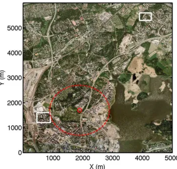
Meteorological and hydrological observations from three ar-eas of Helsinki are used (Fig. 1). At the Kumpula (Ku, SMEAR III) site, both meteorological forcing and evalu-ation data are measured (Järvi et al., 2009a). In addition, the observed runoff from Pasila (Pa) and Pihlajamäki (Pi) catchments are used for model development and evaluation. Kumpula is located 4 km north-east of the Helsinki city cen-tre in a suburban area and 3.8 km from Pa and Pi (Fig. 1). Both Pa and the built sector of Ku (Ku1) have large areas of impervious surfaces (62 %). At both sites, the buildings are mostly offices with mean heights of 15 m (Pa) and 11 m (Ku1). Pasila has pedestrian areas at two heights with exten-sive concrete surfaces creating a complex morphology. The
Figure 1. Aerial photograph of the measurement locations in Helsinki. Red dot is the SMEARIII-Kumpula site (Ku). The red dashed line is the 1 km radius circle that the surface cover frac-tions are calculated for, and the white squares show the approxi-mate locations of the catchment areas (Pa left side and Pi top right).
©Kaupunkimittausosasto, Helsinki, 2011.
other two sectors around the SMEAR III flux tower (Ku2, Ku3) and the Pi catchment are more vegetated (Table 1). Pih-lajamäki, with 34 % impervious surfaces, is a typical subur-ban area in Helsinki with multi-family block houses.
Tower based eddy covariance (EC) sensible and latent heat fluxes measured at 31 m, with an ultrasonic anemome-ter (Metek, USA-1) and a closed-path infrared gas analyser (LI-7000, Li-COR Biosciences, Lincoln, NE, USA) at Ku are used. Post-processing of the 10 Hz data use commonly ac-cepted procedures described in detail in Järvi et al. (2009b) and Nordbo et al. (2012a).
Tower-top air temperature (platinum resistant thermome-ter, Pt-100, “in-house”), wind speed (Thies Clima 2.1x, Goet-tingen, Germany) and incoming and outgoing short- and long-wave radiation (CNR1, Kipp&Zonen, Delft, Nether-lands) are used to force and test the model. Other forcing data measured on a nearby roof (24 m a.g.l.) include air pressure (Vaisala DPA500, Vaisala Oyj, Vantaa, Finland), relative hu-midity (Vaisala HMP243), and precipitation (rain gauge, Plu-vio2, Ott Messtechnik GmbH, Germany). Snow depth mea-sured next to the tower by the Finnish Meteorological Insti-tute is used in the model evaluation.
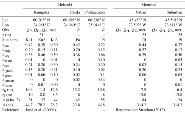
Table 1.Characteristics of the observational sites. Surface cover fractions for the eddy covariance (EC) sites are calculated for 1 km radius circles, whereas the fractions of the catchments are for the actual catchment areas. In Kumpula, the area is divided into three surface cover areas (Ku1, Ku2 and Ku3). For the abbreviations see Appendix C.
Helsinki Montreal
Kumpula Pasila Pihlajamäki Urban Suburban
Lat 60.203◦N 60.199◦N 60.238◦N 45.457◦N 45.501◦N
Lon 24.961◦E 24.940◦E 25.014◦E 73.592◦W 73.811◦W
Obs. Q∗, QH,QE, met. R R Q∗, QH,QE, met. Q∗, QH,QE, met.
z(m) 31 – – 25 25
Site name Ku1 Ku2 Ku3 Pa Pi Rl Pr
λpav 0.42 0.39 0.30 0.42 0.22 0.44 0.37
λbldg 0.20 0.15 0.11 0.20 0.12 0.27 0.12
λveg 0.38 0.46 0.59 0.38 0.66 0.29 0.50
λeverg 0.01 0 0.01 0 0.10 0 0.05
λdec 0.21 0.20 0.30 0.24 0.30 0.03 0.15
λigrass 0.15 0.20 0.21 0.10 0.02 0.20 0.25
λgrass 0.01 0.06 0.10 0.02 0.1 0.06 0.05
λunman 0 0 0 0.02 0.14 0 0
λwater 0 0.01 0.00 0 0 0 0.01
zh(m) 10.4 11.5 12.6 15.2 10.8 7.9 6.4
zt(m) 10 8.8 8.5 8 8 13.0 13.8
p(# ha−1) 31 37 44 42 55 84 24
A(ha) 44.7 78.2 78.2 23.8 44.8 314.2 314.2
Reference Järvi et al. (2009a) – – Bergeron and Strachan (2012)
runoff at unexpected times. Because of the water quality ob-served, this is thought to be associated with pipe leakage in household water systems. From the beginning of September, the excess pipe flow observed was 0.0038 m3s−1which had
increased to 0.0125 m3s−1 by the end of the measurement
campaign. This pipe flow was removed from the analysis when assessing the runoff as pipe leakage is not modelled currently.
2.2.2 Montreal, Canada
Two residential areas with impervious cover of 71 % (Rl, Rosemont-La-Petite-Patrie borough) and 49 % (Pr, Pierrefonds–Roxboro borough) 18 km apart were modelled (see Bergeron and Strachan (2012) for map). The more densely populated Rl has two to three storey buildings, whereas the suburban Pr is a single family house residential area (Table 1).
At both sites, a tower mounted (26 m a.g.l.) sonic anemometer (CSAT3, Campbell Scientific Canada Corp., Edmonton, AB, Canada) and an open-path infrared gas anal-yser (LI-7500, Li-COR Biosciences, Lincoln, NE, USA) pro-vided the 20 Hz data that are post-processed to EC fluxes of sensible and latent heat (Bergeron and Strachan, 2012). Forc-ing data of air temperature and relative humidity (HMP45C-212 at Rl, HMP45C at Pr, Campbell Scientific Canada Corp.), pressure (barometric pressure sensor, RM Young Model 61205V, RM Young Company, Michigan, USA) and
radiation (CNR1) are from the EC tower at 25 m a.g.l. Snow depths were monitored in a back lawn of Pr and on a roof at Rl with snow ranging sensors (SR5, Campbell Scien-tific Canada Corp.). Snow properties, including snow den-sity and albedo, were regularly (weekly: 2007/2008 win-ter or twice every month: 2008/2009 winwin-ter) observed for undisturbed snow, sidewalks, lawns and rooftops. Observa-tions from Coteau-du-Lac (35 km south-west from Pr) and Pierre Elliot Trudeau Airport data (7 km from Pr and 16 km from Rl) (National Climate Data and Information Archive of Canada, 2013) are used to create a precipitation data set with separation of snow/rain.
2.3 Model runs
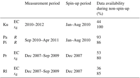
Table 2.Time period and the spin-up time of the model simulations. Data availability refers to the number of 60 min periods when obser-vations are available for the non-spin-up period. EC is the eddy covariance fluxes (QHandQE),Ris the runoff andsdthe snow depth. A
sub-set of these data are used in parameter optimization and another for evaluation.
Measurement period Spin-up period Data availability during non-spin-up (%)
Ku EC 2010–2012 Jan–Aug 2010 44
sd 100
Pa R
Sep 2010–Apr 2011 Jan–Aug 2010 93
Pi R 86
Pr EC Dec 2007–Sep 2009 Dec 2007 53
sd 80
Rl EC Dec 2007–Sep 2009 Dec 2007 36
sd 85
the snow, and surface albedo (Eqs. 3 and 4).QHandQEare
used to test the parameterizations forQMand1Qs,I(Eqs. 5
and 6). The runoff measured in the denser catchment (Pa) is used to constrain the temperature and radiation melt rates (Eq. 6), retention capacity of the snow (Eq. 8) and the limit for the liquid precipitation.Q∗and its components,QHand QE, the snow depth from Ku in 2012 and the runoff from the
medium-intensity catchment are used to independently eval-uate the model.
The meteorological data measured at the Ku site are used to force the model for all three Helsinki sites. The data are gap filled using the procedures described in Järvi et al. (2012). Due to the very different characteristics surround-ing the Kumpula tower, the model is run for the three surface cover areas within a 1 km radius circle. The flux time series evaluated against observations are combined from the surface cover areas (Ku1-3) based on the prevailing wind direction.
In Montreal, only the first of the 22 months (Decem-ber 2007 till Septem(Decem-ber 2009) is used as a spin-up. The short spin-up time is chosen to allow two snowmelt periods in model development and testing. The remainder of the sub-urban data set (Q∗,QH,QE, snow depth, snow density and
albedo) is used for the model development: snow density and albedo are used to determine the shape of the snow aging curves (Eqs. 3, 4 and 9);Q∗, the surface and snow albedo; andQH andQE, the other snow related parameterizations.
The urban site observations are used for independent evalua-tion of the model. The model domain is a 1 km radius circle around the flux tower.
The results are analysed by considering snow-free, cold snow and melting snow periods. For snow-free periods, the simulated snow depth is zero, whereas the cold snow and melting snow periods are separated by the air temperature 0◦C.
2.4 Evaluation statistics
Several statistics are used to evaluate the model performance (e.g. Daley, 1991). Linear regression is used to describe the linear dependence between the independent variable, in this case the observations (XObs), and the dependent variable, the
model output (XMod). The slope (S)relative to 1, and
inter-cept (I )relative to zero, provide information on the model performance. Further, goodness of fit is evaluated using the root mean square error (RMSE):
RMSE=
s P
(XMod(t )−XObs(t ))2
N , (16)
whereN is the number of data points. Like the intercept in the linear regression, the RMSE has the units of the vari-ables being evaluated and it depends on the magnitude of the mean variables. Therefore, it is useful to normalize the RMSE (nRMSE) relative to the range of values observed (Järvi et al., 2011):
nRMSE= RMSE
XObs,max−XObs,min
. (17)
When comparing the performance of the model to simu-late different variables, the RMSE can also be normalized with the standard deviation of the observationsσObs(Taylor,
2001):
sRMSE=RMSE
σObs
. (18)
In addition, the mean bias error (MBE) between the mod-elled and observed time series is considered:
MBE=X X¯Mod− ¯XObs, (19)
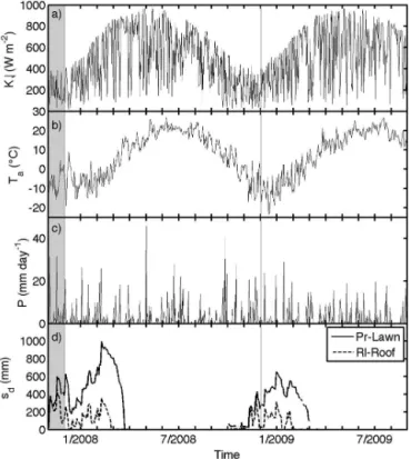
Figure 2.Time series of daily(a)daytime (10:00–14:00) solar ra-diation (K↓),(b)air temperature (Ta),(c)precipitation (P ) mea-sured in SMEAR III – Kumpula, and(d)snow depth measured at Kumpula. The grey area shows the spin-up period.
2.5 General weather conditions
The weather conditions during the modelled period for Helsinki and Montreal are shown in Figs. 2 and 3, respec-tively. Daytime solar radiation exhibits a strong seasonal pat-tern, with the 15◦ latitudinal difference causing more rapid
changes and stronger amplitude in Helsinki than in Montreal. In summer,K↓reaches 970 W m−2in Montreal, whereas in Helsinki, the maxima remain below 830 W m−2. In winter, the solar radiation in Helsinki is very low (<120 W m−2), whereas Montreal peaks are below 400 W m−2. Despite the difference inK↓, air temperatures are fairly similar in both cities. Daily maxima mean temperatures are around 26◦C in
summer, while the minimum daily mean temperature in win-ter in Helsinki is−20◦C and in Montreal−23◦C. In both
cities precipitation is quite evenly distributed throughout the year.
During the 3 years of measurements, the daily snow depths in Helsinki are all below 0.8 m, with a longer snow period in winter 2010/2011 than 2011/2012. The timing of snowpack formation depends strongly on the year. In 2010, it was initi-ated in November, whereas in the following winter this was delayed until January 2012. This will have a large influence not only on both natural energy and water exchanges, but also urban activities. In Montreal, snowpack depth and timing has large variability between years; for example, a 1 m snow pack
Figure 3.As Fig. 2 but for Montreal measured at the suburban site (Pr) with snow depth measured in a suburban back lawn (Pr) and on an urban roof (Rl).
is observed in March 2008 with melting in late April, com-pared to only 0.6 m the next year, with snow melting by the end of March.
3 Results
3.1 Model optimization 3.1.1 Snow properties
Figure 4. Observed and modelled (a) snow density (ρs) and snow albedo (αs)at the suburban site in Montreal (January 2008– April 2009). Observed values are the medians from four locations and the error bars show the quartile deviations. Aging functions pro-posed in Lemonsu et al. (2010) “Le10” and in the current study “New”.
Comparison of these observations with the Lemonsu et al. (2010) (hereafter Le10) aging functions used for the suburban site in Montreal shows that modifications to the coefficients are needed for both snow albedo and den-sity (Fig. 4). The Le10 maximum denden-sity of 350 kg m−3
is too small for the current observations. Thus, the max-imum snow density is set to 400 kg m−3; the minimum
valueρsminis kept at 100 kg m−3. In addition, the time
con-stantτris decreased to 0.043. After these modifications, the
simulated snow density follows the behaviour of the me-dian observations well (Fig. 4a). Similarly from the obser-vations, the minimum (αsmin) and maximum (αmaxs ) snow albedo are set to 0.18 and 0.85, respectively, which dif-fer from Le10 (αnmin=0.15–0.30 across the different sur-face cover types). In Lemonsu et al. (2010) snow albedo aging time constants (τf=0.174, τa=0.008) could not be
fully evaluated due to a lack of data. However, τa
com-pared to our observations is too small. When increased to 0.018,τfdecreases to 0.11. Again, good correspondence
be-tween the observed snow albedo and model output (Fig. 4b), and between the observed and modelled K↑ in Helsinki
in 2012 (not shown) are seen. During the cold snow pe-riod, the linear fit statistics areS=0.68±0.02 W−1m2,I=
0.27±0.47 W m−2 (RMSE=11.3 W m−2, N=2232), and
during the warm snow period S=0.50±0.01 W−1m2and I =0.85±0.47 W m−2 (RMSE=11.4 W m−2, N=604). One likely reason for the poorer model performance during the warm snow period is the sensitivity of the albedo to the fraction of snow covered surface. In the model, the fraction of snow is parameterized based on the maximumSWE, but it
is likely that this is site dependent at a neighbourhood scale
due to redistribution and transport of snow. However, as the other net all-wave radiation components are larger in magni-tude thanK↑, the negative bias during the melting period is
likely to have small impact on the available energy. Melt and freezing factors
The freeze and melt factors (ar and at), representative for
the neighbourhood scale, are optimized using runoff from Pa and snow depth from Ku (Helsinki). SUEWS was run usingarvalues between 0.0008 and 0.002 mm W−1h−1
us-ing 0.0001 mm W−1h−1 resolution, and a
t between 0.05
and 0.15 mm◦C−1h−1 with 0.01 mm◦C−1h−1 resolution.
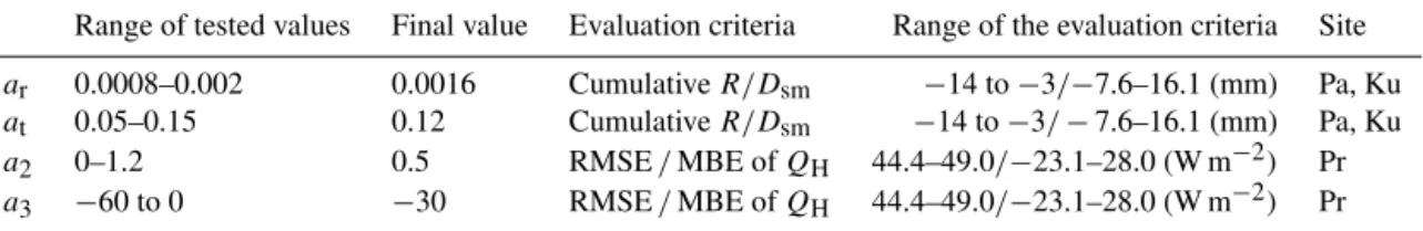
The 146 modelled combinations were analysed with re-spect to the amount of meltwater accumulated during the snow covered period and the timing for complete snowmelt (Table 3). The smallest differences compared to the ob-servations are obtained withar=0.0016 mm W−1h−1 and
at=0.12 mm◦C−1h−1. Thus, these are used in the model
runs. Values are slightly larger, but of the same order of magnitude, than those obtained for hourly factors at an Arctic watershed in Alaska (ar=0.001 mm W−1h−1 and at=0.095 mm◦C−1h−1; Kane et al., 1997). Unfortunately,
no hourly values for urban areas were found in the literature. However, using these factors the daily melt rates are the same order of magnitude as those that have been typically reported for urban areas (Bengtsson and Semádeni-Davies, 2011). Snow storage heat
To determine the storage heat flux coefficientsa1,a2anda3
for snow (Eq. 5), shallow water values were used as an ini-tial basis witha1=0.50,a2=0.21 anda3= −39.1 (Souch
et al., 1998). Given the assumption that the snow heat capac-ity is around half that of water (Rogers and Yau, 1996),a1
is set to 0.25 for snow. The other two coefficients (a2 and a3)are assessed relative to their effect on the sensible heat
flux by running SUEWS for Pr over a range of values during the snow covered period. Pr was chosen to optimize1Qs,I
due to its more homogeneous surface characteristics when compared to other sites. The RMSE between the observed and modelledQHvaries between 44.4 and 49.0 W m−2and
MBE between−23.1 and 28.0 W m−2, whena2 varies
be-tween 0 and 1.2 and a3 between −60 and 0 (Table 3).
The optimal result with minimum RMSE=48.2 W m−2and
MBE=0.19 W m−2 is obtained with a2=0.60 and a3= −30. Thus, these coefficients are used in the model to
cal-culate the snow storage heat or the internal energy of the snow. The values imply a smaller slope or fraction of ra-diative energy entering/leaving (a1), a greater hysteresis (a2)
and a similar phase or time lag (a3)for snow relative to water.
Table 3.Results of the model optimization made for the snow storage heat and meltwater calculations. Different evaluation criteria for the components were used. See text for further explanation.
Range of tested values Final value Evaluation criteria Range of the evaluation criteria Site
ar 0.0008–0.002 0.0016 CumulativeR/Dsm −14 to−3/−7.6–16.1 (mm) Pa, Ku
at 0.05–0.15 0.12 CumulativeR/Dsm −14 to−3/−7.6–16.1 (mm) Pa, Ku
a2 0–1.2 0.5 RMSE/MBE ofQH 44.4–49.0/−23.1–28.0 (W m−2) Pr
a3 −60 to 0 −30 RMSE/MBE ofQH 44.4–49.0/−23.1–28.0 (W m−2) Pr
Figure 5.Modelled and observed runoff at(a)Pa and(b)Pi (in-dependent) sites. The grey line indicates when the snow starts to accumulate on ground; the snowmelts by the end of April.
3.2 Model evaluation
Table 4 lists the parameters, both for the snow covered and snow-free surface, used in the model runs. The snow parame-ters are optimized (Sect. 3.1), whereas the limit values for the snow transport (SWE,Lim)were estimated based on maximum
mass allowances of water at the Pa catchment. The same val-ues were used at all sites as no additional information was available. Sensitivity analyses (Sect. 3.4) suggest the model is fairly insensitive toSWE,Limdespite the expectation for
val-ues to be neighbourhood specific. 3.2.1 Surface runoff
Figure 5 shows the daily observed and modelled runoff from the two catchments in Helsinki. The grey line sepa-rates the non-snow and snow related runoff as the contin-uous winter snow cover formed on 18 November 2010. At both sites, the model simulates the snowmelt induced runoff well, reproducing both the spring melt peak and the reces-sion in April. When the model is run treating the catch-ments as a whole, it tends to overestimate the runoff peaks and to be more peaked than observations (Fig. 5), which have smaller but longer runoff peaks. Partly this can be
explained by the absence of time lags for the water to move from the most distant points (hydrologically and hy-draulically) because the catchment is modelled as one unit (in the current setup). However, in terms of hourly per-formance, the correlation between the observed (Robs)and
modelled (Rmod)runoff is good withS=1.20 (mm h−1)−1
and I= −0.01 mm h−1 (RMSE=0.14 mm h−1, r=0.75)
in Pa, and S=1.24 (mm h−1)−1 and I=0.02 mm h−1
(RMSE=0.16 mm h−1,r=0.60) in Pi. The coefficients are
calculated for periods when both Rmod andRobs are
non-zero (675 and 760 h in Pa and Pi, respectively). In Pa, the model underestimates the cumulative runoff over the snow covered periods by 3 % asRmod=82 mm andRobs=85 mm
(Fig. 6). In Pi, the cumulative runoff is overestimated by 19 % asRmod=97 mm andRobs=81 mm.
Before the continuous snow cover, the model performs similarly at both catchments. Notably, the model overes-timates runoff at Pi with high intensity precipitation. The overestimation is seen in the linear correlation betweenRobs
and Rmod as S=1.29 (mm h−1)−1 and I=0.04 mm h−1
(RMSE=0.20 mm h−1,r=0.68,N=668) as well as in the
modelled cumulative runoff, which is 47 % higher than the observed in Pi (27 and 42 mm, respectively) (not shown). In Pa,S=1.26 (mm h−1)−1(RMSE=0.20 mm h−1,r=0.90,
N=743), and the cumulative runoff is underestimated by
4 % by the model (Robs=84 mm andRmod=88 mm). Some
of these differences are caused by the forcing precipita-tion and other meteorological variables being from the flux site Ku. This would particularly affect the model perfor-mance during convective precipitation, which accounts for 88 % of the precipitation events between April and Septem-ber (Punkka and Bister, 2005).
3.2.2 Snow depth
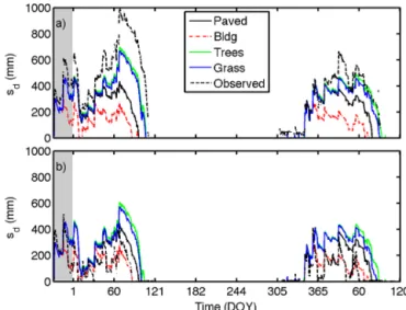
The model calculates snow water equivalent (SWE)and snow
depth (sd)separately for each surface type. Due to snow
re-moval and the different surface characteristics,sd behaves
differently for the vegetated and built surfaces. This can be seen when the modelledsdfor each surface (paved, building,
Table 4.Parameters used in SUEWS for surfaces that are buildings (bldg), pavement (pav), evergreen vegetation (everg), deciduous vegeta-tion (decid), grass and water. If the vegetavegeta-tion is irrigated, different values for describing the canopy are used. Sources of the values are as in Järvi et al. (2011) unless indicated otherwise below. Where different values are used for the different sites, this is indicated for Helsinki (Hel), and for the two sites in Montreal (Rl and Pr). Variable notation is given in Appendix C.
(a) Site Units Bldg Pav Everg. Decid. Irr. veg Grass Water
Si mm 0.25 0.48 1.3 0.3–0.8 1.9 0
Ssoil,i Hel/Rl mm 50 100 150 150 150 150 –
Pr mm 150 150 150 150 150 150 –
D0,i mm 10 10 0.013 0.013 10 0.013 –
b – 3 3 1.71 1.71 0.013 1.71 –
Ci mm 0 0 0 0 0 0 0
Csoil,i HelPr /Rl mmmm 15050 100150 150150 150150 150150 150150 –– αi – 0.15 0.09a 0.10 0.16b 0.19 0.19b 0.08b
εi – 0.95 0.91 0.98 0.98 0.93 0.93 0.95
gi,max mm s−1 – – 7.4 11.7 40 33.1 –
Snow
SWE,0 HelMon mmmm 400 400 400 400 400 400 400
fs,i,0 Hel mm 1 1 1 1 1 1 1
Mon mm 0 0 0 0 0 0 0
ρs,0 kg m−3 120 120 120 120 120 120 120
SmaxWE,i mm 190 190 190 190 190 190 –
SWE,Lim mm 40 100
(b) Overall area parameter values
αmins 0.18 a0,{wd,we} 0.1 W m−2(p−1ha−1)−1i G4 3.36 g kg−1 rescap 10 mm αmaxs 0.85 a1,{wd,we} 9.9×10³W m−2K−1(p−1ha−1)−1 G5 11.07◦C res
drain 0.25 mm h−1 εs 0.99 a2,{wd,we} 0.0102 W m−2K−1(p−1ha−1)−1 G6 0.018 mm RC 1.0 mm
ρe 200 kg m−3 b0,a −84.54 mm GDD 300 S1 0.45 mm
ρsmin 100 kg m−3 b
1,a 9.96 mm K−1 Iw 0 mm S2 15 mm
ρsmax 400 kg m−3 b
2,a 3.67 mm d−1 K↓m 1200 W m−2 SPipe 100 mm
τa 0.018 b0,m −25.36 mm Ks 0.0005 mm s−1 SDD −450
τf 0.11 b1,m 3.00 mm K−1 LAImax,everg 5.1 m2m−2 TBaseGDD 5◦C
a1 0.25 b2,m 1.10 mm d−1 LAImax,
dec 5.5 m2m−2 TBaseSDD 10◦C
a2 0.6 CRmin 0.05 mm LAImax,grass 5.9 m2m−2 TBaseQF 18.2◦C
a3 −30 CRmax 0.2 mm LAImin,everg 4.0 m2m−2 Tlim 2.2◦Cc
af 1 G1 16.48 mm s−1 LAImin,dec 1.0 m2m−2 TH 40◦C
ar 0.0016 mm W−1h−1 G2 566.1 W m−2 LAImin,grass 1.6 m2m−2 TL 10◦C at 0.011 mm◦C−1h−1 G3 0.216 kg g−1 rs,max 9999 s m−1 Tstep 300 s
aOptimized using data from Helsinki;bVargo et al. (2013);bAuer (1974).
types at the neighbourhood scale. Thus, some differences be-tween the modelled and observedsdare expected.
In Helsinki, the point observations are made in an open space that corresponds most appropriately to the modelled grass surface. Data for 2011 and 2012 are plotted separately as the first year is used in the model parameter determina-tion, whereas the latter is an independent data set (Fig. 7). In both years, the model reproduces the accumulation of snow and melt events well, but underestimates the snow depth by 84 mm on average compared to the observations. The mea-sured maximum snow depth in 2011 is 720 mm, whereas the
modelled snow depth above grass is 587 mm. Similarly, for 2012 the observed depth is 630 mm and the modelled value is 504 mm. This underestimation is caused by either the un-derestimation of modelledSWEor by overestimation of snow
Figure 6. Modelled and observed cumulative runoff during the snow covered period (19 November 2010–31 April 2011) (a)Pa
and(b)Pi (independent) catchments.
Figure 7.Simulated (by surface type) and observed snow depth in Helsinki in(a)2011 and(b)2012. The grey area shows the spin-up period.
in 2012 the snowmelt finished on 12 April, 1 day later than modelled.
For Montreal,sdis calculated separately for the suburban
(Pr) and urban (Rl) sites for January 2008–April 2009. In Pr, the observations are made on a lawn corresponding to the modelled grass surface (Fig. 8a). The model follows the accumulation and melt events well, but like Helsinki, snow depths are underestimated, especially in the 2007–2008 win-ter. The maximum observed sdis 1020 mm, while 670 mm
was modelled for grass. In winter 2008–2009, the maximum observed and simulated snow depths are 665 and 460 mm. In 2008, the modelled snow starts to accumulate on the same day (8 December) as observed. Snowmelt is completed on
Figure 8.As Fig. 7 for Montreal in 2008–2009(a)suburban site with observations above (grass) lawn and(b)urban site with (build-ing) roof observations. The grey area shows the spin-up period.
20 April 2008, which is 3 days after the modelled date. In 2009, the modelled snowmelt finishes 1 day before observed (30 March).
In Rl, sd is observed on a building roof. This has both
lower snow amounts and earlier melt compared to the lawn observations in Montreal (Fig. 8b). The model simulates this behaviour well, but again underpredicts the depths. The ob-servedsdmaxima are 390 and 415 mm for the two winters,
while 301 and 285 mm are modelled, respectively. Accumu-lation of snow takes place on the correct day in Rl, and the snowmelts on the same day as observed (26 March) in 2008, and 9 days later (7 March) in 2009 than observed.
The underestimation of sd is also impacted by the
pre-cipitation measurements, as the difference between observed and modelled values begins during the snow accumulation period. Precipitation measurements are known to underesti-mate snowfall, especially due to wind effects (Goodison et al., 1998; Savina et al., 2012).
3.2.3 Turbulent and radiative energy fluxes
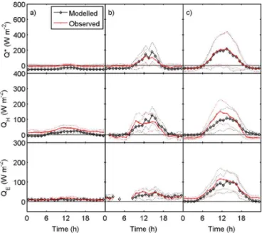
The simulatedQ∗,QH andQE are assessed for snow-free,
cold snow and warm snow periods (Table 5, Fig. 9), with the diurnal behaviour of both the observed and modelled fluxes for the independent data sets in Helsinki and Montreal con-sidered (Figs. 10 and 11).
Generally, the best simulated flux of the three isQ∗
inde-pendent of whether there is snow on the ground or not. For the cold and warm snow periods, the RMSE varies between 27–41 W m−2 (nRMSE=0.037–0.061) and 31–41 W m−2 (nRMSE=0.041–0.057) across the sites. At all sites,Q∗is underestimated in cold snow conditions with MBE between
Figure 9.Model performance for(a)Q∗,(b)QHand(c)QEduring the cold snow, warm snow and snow-free periods. Mean bias error
(MBE) versus normalized root means square error (nRMSE) for different sites and for Ku separately (years 2011 (Ku11)) and 2012(Ku12)).
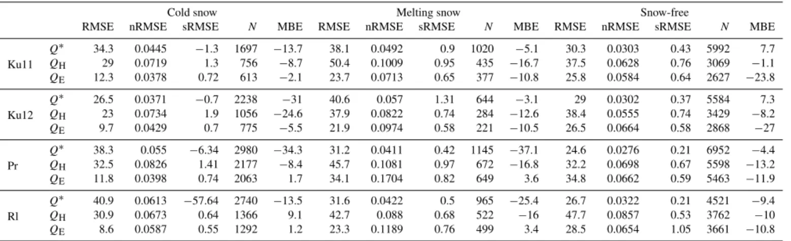
Table 5. Model evaluation statistics based on performance relative to observations of net all-wave radiation (Q∗, W m−2), sensible (QH, W m−2)and latent heat fluxes (QE, W m−2)undertaken for 2 years at one site in Helsinki (Ku11 for 2011 and Ku12 for 2012) and 1 year for two sites in Montreal (Pr and Rl). The statistics: RMSE is the root mean square error (W m−2), nRMSE the normalized RMSE (Eq. 17), sRMSE (Eq. 18) is RMSE normalized with standard deviation of the observed value andNis the number of points in the linear fit.
Cold snow Melting snow Snow-free
RMSE nRMSE sRMSE N MBE RMSE nRMSE sRMSE N MBE RMSE nRMSE sRMSE N MBE
Ku11
Q∗ 34.3 0.0445 −1.3 1697 −13.7 38.1 0.0492 0.9 1020 −5.1 30.3 0.0303 0.43 5992 7.7 QH 29 0.0719 1.3 756 −8.7 50.4 0.1009 0.95 435 −16.7 37.5 0.0628 0.76 3069 −1.1 QE 12.3 0.0378 0.72 613 −2.1 23.7 0.0713 0.65 377 −10.8 25.8 0.0584 0.64 2627 −23.8
Ku12
Q∗ 26.5 0.0371 −0.7 2238 −31 40.6 0.057 1.31 644 −3.1 29 0.0302 0.37 5584 7.3
QH 23 0.0734 1.9 1056 −24.6 37.9 0.0822 0.74 284 −12.6 38.4 0.0555 0.74 3429 −8.2 QE 9.7 0.0429 0.7 775 −5.5 21.9 0.0974 0.58 221 −10.5 26.5 0.0664 0.58 2868 −27
Pr
Q∗ 38.3 0.055 −6.34 2980 −34.3 31.2 0.0411 0.42 1145 −37.1 24.6 0.0276 0.21 6952 −4.4 QH 32.5 0.0826 1.41 2177 −8.4 45.7 0.1081 0.97 672 −16.8 32.2 0.0698 0.67 5598 −13.2 QE 11.8 0.0398 0.74 2063 1.7 34.1 0.1704 0.82 649 3.6 34.8 0.0662 0.59 5463 −11.9
Rl
Q∗ 40.9 0.0613 −57.64 2740 −13.5 31.6 0.0422 0.5 965 −25.4 26.7 0.0322 0.21 4521 −9.4
QH 30.9 0.0673 0.64 1366 9.1 42.7 0.088 0.68 522 −16 47.7 0.0857 0.53 3762 −10
QE 8.6 0.0587 0.55 1292 1.2 23.3 0.1189 0.76 499 3.4 28.5 0.0654 1.05 3661 −10.8
from air temperature and relative humidity (Loridan et al., 2011 – who suggest that use of cloud cover data as input with this technique is better). This parameterization works less well in cold conditions than above 0◦C. In Montreal,
the warm snow underestimation is even larger (MBE= −37
to −25 W m−2), compared to Helsinki where the underes-timation decreases to −5 to −3 W m−2. Especially during
the warm snow periods, the fraction of snow cover plays an important part in the model performance. It affects both the snow albedo and outgoing long-wave radiation via surface temperature. The best performance forQ∗is under snow-free conditions, when the MBE is between−10 and 8 W m−2and the nRMSE is clearly lower than for the periods with snow cover (Fig. 9a).
The scatter in the model performance is larger forQEthan
for the other energy balance components, with cold snow periods having the best, and warm snow periods the poorest model performance (Fig. 9c). The RMSE during cold snow varies between 9–12 W m−2 (nRMSE=0.038–0.059), and
for warm snow between 22–34 W m−2 (nRMSE=0.071–
0.170). The increase in RMSE during warm snow peri-ods is understandable as the energy consumed in melting snow and freezing meltwater is higher and thus errors in
the degree-day-method propagate more easily toQE(as well
as toQH). During melting periods there can be advection
from snow-free surfaces to the snowpack altering the energy balance as specified in Eq. (1) (Bengtsson and Semádeni-Davies, 2011). MBE varies between−11 and 4 W m−2when
there is snow on ground. During snow-free periods, the model underestimatesQE at all sites with MBEs between −27 and −11 W m−2, RMSEs between 26 and 35 W m−2
and nRMSE between 0.058 and 0.066.
In SUEWS,QHis calculated as a residual from other
en-ergy fluxes; therefore, the net error accumulates inQH.
De-spite this, the model is able to simulate its behaviour well. When there is snow on ground, the RMSE varies between 23 and 50 W m−2and nRMSE between 0.067 and 0.118. During the cold snow periods, the simulated heat fluxes are slightly better than during warm snow periods, similar toQE. The
model overestimates QH during snow cover, except in Rl
during cold snow periods, and MBEs vary between−25 and
9 W m−2. In summer, the performance of the model in
Figure 10. Diurnal behaviour of the measured and modelled net all-wave radiation (Q∗)and turbulent energy fluxes (QHandQE) during(a)cold snow,(b)melting snow and(c)snow-free periods in Helsinki in 2012. Only hours when observations are available were accounted for. Dotted lines show the quartile deviations.
The model performance for the energy fluxes is more de-pendent on the period of analysis than the site where it is run. An exception to this isQHat R1, where the model
overesti-mates and shifts the diurnal peak flux earlier compared to the observations (Fig. 11). This appears whether there is snow on ground or not, suggesting that this is caused by the snow-free storage heat flux which is underestimated by the model or anthropogenic heat flux, which is overestimated. RMSEs obtained for the warm snow periods in Pr are higher than Le10 obtained for the same suburban area in Montreal using the Town Energy Balance model in spring 2005. However, direct comparisons are difficult as in their 1 month of obser-vations snow cover is present only on some days compared to the longer time period evaluated here.
3.3 Energy balance of urban snow covered surface Snow cover and the related energy storage and the energy related to phase change alter the surface energy balance. The components at the most built-up site Rl are evaluated here (Fig. 12). During cold snow periods, the daytime en-ergy balance is dominated by the net all-wave radiation (Q∗)
and the sensible heat flux (QH), reaching 119 W m−2 and
113 W m−2. Q
H is fuelled by both Q∗ and QF (reaching
46 W m−2), and it accounts on average for 68 % of the day-time (10:00–15:00 LT) available energy. The dominance of Q∗andQHare typical also for natural cold snow packs (e.g.
Oke, 1987). Only 12 % ofQ∗+QFis dissipated by
evapo-ration, whereas the storage fractions are 10 and 8 % at the snow and snow-free surfaces, respectively. At night, on the
other hand, the urban surface loses long-wave radiation caus-ing the internal energy of the snow to decrease, that is, the cold content of the snow increases. At the same time, the snow-free surface loses some energy (around 10 W m−2)and
bothQFandQEremain positive (by more than 10 W m−2),
withQHless than 5 W m−2.
During warm snow periods,Q∗ is clearly the most im-portant component of the surface energy balance reaching 200 W m−2 in daytime. Now the daytime QF is slightly
smaller than during the cold periods reaching 35 W m−2. Most of the energy, but clearly less than during the cold snow period, is partitioned toQH (46 %), with the second largest
contribution going to snow-free surface heat storage (29 %). Evaporation consumes 17 % of the energy, and only 4 % and 3 % is stored in the snow and consumed by snowmelt. The largestQH and 1QS are consistent with the observations
obtained by Le10 at the suburban site, although they docu-mented a larger contribution going to snow related processes than to evaporation. Moreover, the modelled fractions during the snow covered periods are of the same order of magnitude as obtained for observations at the same site (Bergeron and Strachan, 2012).
When the ground is free of snow, most energy (Q∗+QF)
again goes toQH (188 W m−2, 45 %) followed by the
stor-age heat flux (175 W m−2, 42 %). Due to the high impervious nature of the surface, daytimeQEreaches 50 W m−2, which
is only 12 % of the available energy. The resulting daytime Bowen ratio (QH/QE)is 3.7, which corresponds well with
the expected relationship of the Bowen ratio with the site’s vegetation fraction (Loridan and Grimmond, 2012).
3.4 Model sensitivity
To better understand the impact of both the optimized values and those estimated (Table 4) without detailed observation on the model performance, sensitivity analyses were under-taken. The analysis included the power of the vegetation de-pletion curve (Eq. 15a), limit for the transport of snow from paved and building surfaces (SWE,Lim), snow heat storage
(a2,a3)and the meltwater coefficients (ar,at). SUEWS was
run using the three independent datasets (Ku in 2012, Rl and Pi) changing the parameters by ±30 % using a 10 % step.
The results were compared to hourly measuredQH,QEand
runoff and the RMSE determined for each site and variable (Fig. 13). The other parameters were held constant during each set of analyses.
The impact of the coefficients on heat storage in snow pack is shown only forQHas their effect onQEand runoff is small
or non-existent.SWE,Lim and the meltwater coefficients have
Figure 11.As Fig. 10, for the urban site in Montreal (Rl) in 2008– 2009.
Figure 12.Modelled energy balance at the urban site (Rl) in Mon-treal during(a)cold snow,(b)warm snow and(c)snow-free peri-ods.Q∗=net all-wave radiation,1QS=heat storage to snow-free surfaces, QF=anthropogenic heat flux,QH=sensible heat flux, QE=latent heat flux,QM=snowmelt/freezing water related en-ergy flux and1QI=heat storage in snow pack.
(Grimmond et al., 2011) indicating that the model is fairly insensitive to changes in the studied parameters.
4 Conclusions
The Surface Urban Energy and Water Balance Scheme (SUEWS) is developed to simulate the energy and water
Figure 13.Boxplot of RMSE’s of the sensitivity analysis made for
(a)QH in Ku (W m−2), (b) QE in Ku (W m−2), (c)QH in Rl
(W m−2),(d)QE in Rl (W m−2)and(e)runoff in Pi (mm h−2). The sensitivity are to changes in: the power in the depletion curve (Eq. 15a) (C1),SWE,Lim (C2), meltwater coefficients (ar, at)(C3) and storage heat flux coefficients (a2, a3)(C4). The final model values are indicated (*). For other details see text.
balances in cold climate cities with special attention on the simulation of snow cover. The new model considers the ac-cumulation of snow, snow properties including snow wa-ter equivalent, snow depth, snow density and albedo and snowmelt and refreezing of meltwater based on an hourly degree-day method. The development and independent eval-uation is undertaken using observations from three sites in Helsinki and two sites in Montreal. Each of these sites varies in terms of surface cover characteristics. In Helsinki, the ob-servations include stormwater runoff from two catchments and turbulent fluxes of sensible and latent heat from one site. In Montreal, the observations include snow properties as well as the turbulent fluxes at both sites.
The model developments include an improved description of vegetation phenology (LAI) in cold climate cities. The leaf-off period based on daily air temperature was acceler-ated using a combination of daily air temperatures and day length. Updated aging functions for snow density and albedo in urban areas were developed based on snow observations in Montreal; an improved equation for the degree-day method was used to calculate snowmelt and freezing of the melted water; and new parameter values were developed to calcu-late the snow storage heat flux using the objective hysteresis model (OHM).
uncertainties in determining the snow covered surface frac-tions, as well as the propagating uncertainties from the cal-culation of melt and freezing related energies based on the degree-day method.
Appendix A: Leaf area index (LAI)
In SUEWS, changes in phenology, such as growing season length, are allowed to vary from year to year as a function of thermal conditions through growing degree days and senes-cence degree days. The thermal thresholds are changed to be appropriate for a location (e.g. latitude, continental vs. mar-itime climate) (Järvi et al., 2011). At high latitudes, air tem-perature is a good proxy for leaf growth in spring, whereas the leaf-off is initiated by day length (Keskitalo et al., 2005). However, air temperature still influences the rate of leaf fall. Thus the functions to calculate daily leaf area index (LAId,i)
are modified to also take the day length into account accord-ing to
LAId,i= LAIbd1−1,iGDD·c1+LAId−1,
leaf−on, Td>TBaseGDD LAId,i= LAIbd2−1,iSDD·c2+LAId−1,
leaf−off, Td<TBaseSDD,or
LAId,i= LAId−1,ib3(1−GDD)·c3+LAId−1,
leaf−off, td<12 h
(A1)
where GDD and SDD are the growing and senescence de-gree days, b1,2,3 and c1,2,3 control the rate of change in
LAI and TBaseGDD and TBaseSDD are the base temperature
for senescence. Using the original LAI functions with co-efficientsb1=b2=0.03 andc1=c2=5×10⁻⁴resulted in
too-slow both leaf-on and leaf-off periods in both cities when compared to visual inspection. Thus, for the leaf-on period, the coefficients at both cities were changed to b1=0.04
and c1=0.001, and the new senescence parameterization
(Eq. 20) based on the day length with parametersb3= −1.5
andc3=1.5×10⁻³ was deployed. Unfortunately no
mea-surements of LAI were available. The values are from visual surveys of leaf-on and leaf-off timings.
Appendix B: Snow fraction depletion curves for vegetated, paved and building surfaces
Appendix C: Notation used
αi Effective surface albedo (–) αs Effective snow albedo (–) αsmin Minimum snow albedo (–) αsmax Minimum snow albedo (–)
1Q∗ Change in the net all-wave radiation in time step1t(W m−2)
1QA Advective heat flux (W m−2)
1Qs,I Change in the snow heat storage (W m−2) 1SWE Change in the snow water equivalent
(mm h−1)
1t Time step of the model (s) εi Effective surface emissivity (–)
εs Effective surface emissivity of snow (–) γ Psychrometric constant (Pa◦C−1) λbldg Surface fraction of buildings (–) λdec Surface fraction of deciduous trees (–) λev Surface fraction of evergreens (–) λgrass Surface fraction of non-irrigated grass (–) λigrass Surface fraction of irrigated grass (–) λpav Surface fraction of paved areas (–) λunman Surface fraction of unmanaged land (–) λveg Surface fraction of vegetation (–) λwater Surface fraction of water (–) ρ Air density (kg m−3)
ρe Threshold value in the calculation of
reten-tion capacity (kg m−3) ρs Snow density (kg m−3) ρs,0 Initial snow density (kg m−3) ρw Water density (kg m−3)
ρmaxs Maximum snow density (kg m−3) ρmins Minimum snow density (kg m−3)
τa Cold snow time constant for snow albedo
aging (–)
σObs Standard deviation of observed values τd Seconds in 1 hour (3600 s h−1)
τf Warm snow time constant for snow albedo
aging (–)
τh Period of 1 day (86 400 s)
τr Time constant describing the snow density
aging (–)
a0,{wd,we} Parameter defining the baseQfper capita
(W m−2(capita−1ha−1)−1)
a1,{wd,we} Parameter related to CDD (W m−2K−1
(capita−1ha−1)−1)
a2,{wd,we} Parameter related to HDD (W m−2K−1
(capita−1ha−1)−1)
a1,2,3 Constants in the calculation of the snow
heat storage
ar Radiation melt factor (mm W−1h−1) at Temperature melt factor (mm◦C−1h−1) af Temperature freezing factor
(mm◦C−1h−1)
A Study area (ha)
b Empirical coefficient in the calculation of drainage
b1,2,3 Parameters controlling the speed of leaf on b0a,1a,2a Parameters for automatic irrigation
(mm, mm K−1, mm d−1)
b0m,1m,2m Parameters for manual irrigation (mm,
mm K−1, mm d−1)
bldg Building surface type
c1,2,3 Parameter to control the speed of leaf-off cp Heat capacity of air (J kg−1K−1)
cw Specific heat capacity of water
(kJ kg−1◦C−1)
Ci Interception state ofith surface (mm) Csoil,i Soil water storage (mm)
CR Retention capacity (mm)
CminR Minimum retention capacity (mm) CmaxR Maximum retention capacity (mm)
d Day
D0,i Drainage rate (mm) Dsm Day of the snowmelt
decid Deciduous surface type E Evaporation (mm h−1)
EC Eddy covariance
everg Evergreen surface type fs,i Fraction of snow on surface fs,i,0 Initial fraction of snow
F Freezing water on surface (mm h−1) gi,max Maximum conductance (m s−1)
G1−6 Parameters related to surface conductance
GDD Growing degree days i Surface type index irr. veg. Irrigated vegetation type I Interception of linear regression
Iw Additional water to water surface type
(mm)
K↓ Downward shortwave radiation (W m−2) K↓m Maximum incoming solar radiation used in
gscalculation
K↑ Upward shortwave radiation (W m−2) Ks Saturated hydraulic conductivity (mm s−1)
Ku Kumpula site
Ku1 Built sector at the Kumpula site Ku2 Road sector at the Kumpula site Ku3 Vegetation sector at the Kumpula site Lf Latent heat of fusion (J kg−1)
LAId,i Daily leaf area index (m2m−2)
LAImax,i Maximum LAI of surface typei(m2m−2)
Lat Latitude (◦)
Lon Longitude (◦)
LUMPS Local-scale Urban Meteorological Param-eterization Scheme
M Snowmelt and re-freezing of melted water (mm h−1)
MBE Mean biased error
nRMSE Normalized root mean square error N Number of data points
NARP Net all-wave radiation Parameterization Scheme
OHM Objective hysteresis model
p Population density inside the grid (capita ha−1)
P Precipitation (mm h−1) Pa Pasila site
Pav Paved surface type Pi Pihlajamäki site
Pr Pierrefonds–Roxboro site Q∗ Net all-wave radiation (W m−2) QA Advective heat flux (W m−2) QE Latent heat flux (W m−2)
QF Anthropogenic heat flux (W m−2) Qg Ground heat flux (W m−2) QH Sensible heat flux (W m−2)
QM Energy consumed to melt snow (W m−2) Qp Heat released from rain on snow (W m−2) r Pearsons correlation coefficient
ra Aerodynamic resistance (s m−1) rs,max Maximum surface resistance (s m−1)
rescap Surface water capacity in LUMPS (mm)
resdrain Drainage rate of water bucket in LUMPS
(mm h−1) R Runoff (mm h−1)
RC Limit when surface is totally covered with
water in LUMPS (mm) Rl Rosemont-La-Petite-Patrie site Rmod Modelled runoff (mm) Robs Observed runoff (mm)
RMSE Root mean square error
s Slope of the saturation vapour pressure curve over ice (Pa◦C−1)
sd Snow depth (m)
sRMSE RMSE normalized with standard deviation of the observation
S Slope of linear regression
S1−2 Parameters related to surface conductance Si State of the snow-free surface (mm) SPipe Maximum depth capacity of pipes (mm) Ssoil,i Soil state (mm)
SWE Snow water equivalent (mm) SWE,0 Initial snow water equivalent (mm) SWE,Lim Limit of the snow water equivalent for
snow removal (mm)
SmaxWE,i Snow water equivalent when surface typei is fully covered with snow (mm)
SDD Senescence degree days
SMEAR III Station for Measuring Ecosys-tem/Atmosphere Relations
SUEWS the Surface Urban Energy and Water Bal-ance Scheme
t Current time step
td Day length (h)
Ta Air temperature (◦C)
TBaseGDD Base temperature for leaf growth (◦C) TBaseSDD Base temperature for senescence (◦C) TBaseQF Base temperature forQF(◦C)
TH,TL Parameters related to calculation ofgs(◦C) Tlim Temperature limit for the liquid
precipita-tion and snow (◦C)
Ts Snow surface temperature (◦C)
TStep Time step for water balance calculation(s) TR Transport of snow from the study area
(mm)
unman Unmanaged surface area V Vapour pressure deficit (Pa) veg Vegetaed surface area XMod Modelled variableX
XMod, max Maximum value of observed time series XObs Observed variableX
XObs, max Maximum value of observed time series z Height of the meteorological
measure-ments (m)
z0v Roughness length for heat and water
vapour (m)
z0m Roughness length for momentum (m) zh Mean building height (m)