www.the-cryosphere.net/8/329/2014/ doi:10.5194/tc-8-329-2014
© Author(s) 2014. CC Attribution 3.0 License.
The Cryosphere
What drives basin scale spatial variability of snowpack properties in
northern Colorado?
G. A. Sexstone and S. R. Fassnacht
ESS-Watershed Science Program, Warner College of Natural Resources, Colorado State University, Fort Collins, Colorado 80523-1476, USA
Correspondence to:G. A. Sexstone ([email protected])
Received: 23 April 2013 – Published in The Cryosphere Discuss.: 18 June 2013 Revised: 27 January 2014 – Accepted: 30 January 2014 – Published: 3 March 2014
Abstract.This study uses a combination of field
measure-ments and Natural Resource Conservation Service (NRCS) operational snow data to understand the drivers of snow den-sity and snow water equivalent (SWE) variability at the basin scale (100s to 1000s km2). Historic snow course snowpack density observations were analyzed within a multiple lin-ear regression snow density model to estimate SWE directly from snow depth measurements. Snow surveys were com-pleted on or about 1 April 2011 and 2012 and combined with NRCS operational measurements to investigate the spatial variability of SWE near peak snow accumulation. Bivariate relations and multiple linear regression models were devel-oped to understand the relation of snow density and SWE with terrain variables (derived using a geographic informa-tion system (GIS)). Snow density variability was best ex-plained by day of year, snow depth, UTM Easting, and el-evation. Calculation of SWE directly from snow depth mea-surement using the snow density model has strong statisti-cal performance, and model validation suggests the model is transferable to independent data within the bounds of the original data set. This pathway of estimating SWE directly from snow depth measurement is useful when evaluating snowpack properties at the basin scale, where many time-consuming measurements of SWE are often not feasible. A comparison with a previously developed snow density model shows that calibrating a snow density model to a specific basin can provide improvement of SWE estimation at this scale, and should be considered for future basin scale analy-ses. During both water year (WY) 2011 and 2012, elevation and location (UTM Easting and/or UTM Northing) were the most important SWE model variables, suggesting that oro-graphic precipitation and storm track patterns are likely
driv-ing basin scale SWE variability. Terrain curvature was also shown to be an important variable, but to a lesser extent at the scale of interest.
1 Introduction
A majority of earth’s moving freshwater originates in snow-dominated mountainous areas (Viviroli et al., 2003), with 60 to 75 percent of annual streamflow in the Rocky Mountain re-gion of the western United States originating from snowmelt (Doesken and Judson, 1996). A comprehensive understand-ing of the distribution of the seasonal mountain snowpack and estimation of its snow water equivalent (SWE) is essen-tial to improve hydrologic models used for forecasting wa-ter availability. Additionally, the recent shift towards earlier snowmelt in regions of the western US (e.g., Stewart, 2009; Clow, 2010) necessitates a more accurate accounting for fu-ture water resources planning. Mountainous landscapes have complex topography as well as strong and highly variable cli-matic gradients, yielding spatial and temporal (seasonal and interannual) variability in snowpack properties. Determining the meteorology and related feedbacks that drive hydrologic processes in these areas is challenging, as the resolution of available SWE measurements is often much coarser than the scale needed to characterize the correlation length of its spa-tial variability (Blöschl, 1999), and requires spaspa-tial scaling (Bales et al., 2006).
can be calculated at a daily and monthly time step, respec-tively. Hourly SNOTEL data are also available, but were not used in this study. NRCS operational stations were estab-lished to measure the snowpack for water supply forecasts, yet, they have been shown to represent SWE only as a point location rather than surrounding area (Molotch and Bales, 2005). Nonetheless, SNOTEL and snow course sites are the most widely available and utilized ground-based measure-ments of SWE and relied upon heavily for estimating basin scale snow distribution.
Research on the spatial distribution of snow has empha-sized the statistical relation between snow properties and ter-rain characteristics, the latter as a surrogate for the driving meteorology. These studies have used SNOTEL data to inter-polate SWE over large basins (e.g., Fassnacht et al., 2003), as well as manual field snowpack measurements over small catchments (e.g., Elder et al., 1991). However, few studies have analyzed snow’s spatial variability at the basin scale using both operational and field-based measurements. Op-erational measurements can provide regional knowledge on the spatial distribution of snow (e.g., Fassnacht et al., 2003), yet cannot accurately characterize the basin scale variabil-ity that vitally impacts snowmelt and runoff (Bales et al., 2006). It has been recommended that future research should focus on more accurate estimation of SWE at the basin (100s to 1000s km2)and regional (10 000s to 100 000s km2)scale to effectively assess and manage mountain water resources (Viviroli et al., 2011). There is a need to supplement oper-ational data with additional field-based snowpack measure-ments at this scale of interest to evaluate the spatial vari-ability of SWE and provide additional ground-truth measure-ments within the scale extent of remote sensing observations. At the basin scale, an approach to reducing the sampling effort is to use snow depth as a surrogate for SWE by de-veloping a model for snow density, as manual snow density measurements require more time and effort than snow depth measurements. Recent studies have attempted to character-ize the spatiotemporal characteristics of snow density (e.g., Mizukami and Perica, 2008; Fassnacht et al., 2010), or to de-velop reliable methods for modeling snow density and thus estimating SWE from snow depth measurements (e.g., Jonas et al., 2009; Sturm et al., 2010).
The objectives of this research were (1) to evaluate basin scale snow density variability from historic snow course measurements and develop a snow density model specific to our study area that can be used to estimate SWE from snow depth measurements; this is a different domain and scale than used in previous studies, and (2) to combine operational SNOTEL and snow course measurements, as suggested by Dressler et al. (2006), with supporting field-based snowpack measurements to evaluate what is driving variability of the snowpack at the basin scale.
2 Study area and datasets
This study was conducted in the Cache la Poudre Basin lo-cated in the Front Range of northern Colorado and a small portion of southeastern Wyoming (Fig. 1). We focus on the portion of this basin that shows persistent snow cover near peak snow accumulation; this region is responsible for the majority of hydrologic input to the river system. To de-fine this area, we use the Snow Cover Index (SCI) at 50 % (Richer et al., 2013), which represents the area that was snow-covered at least 50 % of the time from 2000 to 2010 during early April. The SCI is calculated based on the Mod-erate Resolution Imaging Spectroradiometer (MODIS)/Terra 8-day snow cover products. The portion of the basin within the 50 % SCI has an area of 1493 km2and ranges in eleva-tion from 2040 to 4125 m. Spruce-fir (Picea engelmanniiand
Abies lasiocarpa), lodgepole pine (Pinus contorta), and pon-derosa pine (Pinus ponderosa) forests cover a majority (ap-proximately 77 %) of this area, with the alpine community located at the highest elevations and the mountain shrub com-munity located at the lowest elevations. Snow is the dominant form of precipitation within the basin, and the hydrograph peak is driven by snowmelt generally occurring in late May to June. The majority of winter moisture moves into this re-gion by Pacific frontal storm tracks from the west, southwest, or northwest, however, systems moving north from the Gulf of Mexico can also bring substantial snowfall to the Front Range of Colorado (Barry, 2008).
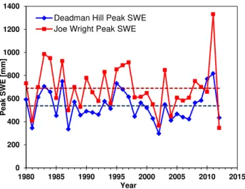
The NRCS operational stations located within the study area and in a 15 km buffer around the basin were analyzed (Fig. 1), yielding a total of 10 SNOTEL stations and 17 snow courses. Deadman Hill and Joe Wright, the two long-term SNOTEL stations located within the Cache la Poudre Basin, have a mean (1980 to 2012) peak SWE of 538 mm and 690 mm, respectively (Fig. 2). The lowest snow year recorded was 2002 at Deadman Hill and 2012 at Joe Wright, while the maximum snow year was 2011 at both SNOTEL stations. Despite the similar elevation of the two stations, his-torically Joe Wright (3085 m) has a greater accumulation of snow than Deadman Hill (3115 m).
Fig. 1.The Cache la Poudre Basin located in the northern Front Range of Colorado, USA. The study area is represented by the 50 % Snow Cover Index (SCI) which is indicated by the transparent light gray color within the basin. The locations of operational and field-based snow measurements are shown, including a detailed sampling diagram of one systematic field-based sampling transect.
0 200 400 600 800 1000 1200 1400
1980 1985 1990 1995 2000 2005 2010 2015
Pe
a
k
SWE
[m
m
]
Year
Deadman Hill Peak SWE Joe Wright Peak SWE
Fig. 2.Annual peak SWE and mean annual peak SWE (1980 to
2012) for Deadman Hill and Joe Wright SNOTEL stations.
snowpack was less than 50 cm. A cylindrical plastic snow sampling tube with a diameter of 6.6 cm was used to mea-sure snow density for snowpacks greater than 50 cm and less than 150 cm. Additionally, a Federal Sampler (diameter of
measurements to standardize the field-based snow depth measurements to a single date for each survey. The average change in snow depth among SNOTEL stations was added to our field-based snow depth measurements outside of the standardized date to adjust for the change in snow depth over that period. Snow depth measurements from the 2011 survey were standardized to 2 April, while 2012 measurements were standardized to 31 March.
3 Background and methods
3.1 Snow density model
SWE, in millimeters, is the product of snow depth (ds) mea-sured in meters and snow density (ρs)in kilograms per cu-bic meter. At operational sites, the seasonal variability of snow density is largely dictated by time of year, and inter-annual variability is typically low (Mizukami and Perica, 2008). However, previous spatial snow surveys have shown that snow density can exhibit inter-annual variability, par-ticularly in continental regions (e.g., Balk and Elder, 2000; Jepsen et al., 2012). Snow density tends to increase gradually throughout the snow season due to crystal metamorphism, settling, and compaction. Therefore, snow density tends to increase with the day of year (Mizukami and Perica, 2008) and with increasing snow depth (Pomeroy and Gray, 1995). Elevation has also been shown to influence snow density, with the effect often being dependent on the day of year (e.g., Jonas et al., 2009). Topography and tree canopy also impact snow densification, as they can be surrogates for solar radi-ation. However, large datasets of snow density are rare, and not often meant to represent varying terrain and canopy con-ditions, which limits the ability of these data to represent the variability explained by those variables. Since the range of variability of snow density is more conservative than snow depth and SWE (e.g., Logan, 1973; Fassnacht et al., 2010), estimating density from depth has been shown to provide a reasonable pathway for estimating SWE from a snow depth measurement. Based on the approaches presented by Jonas et al. (2009) and Sturm et al. (2010) we have analyzed his-toric operational snow density data for the Cache la Poudre Basin to develop and evaluate a snow density model. We ac-knowledge that the operational snow density data evaluated are not representative of potential terrain and canopy controls on the variability of snow density at the basin scale. However, the potential drivers of snow depth, time of year, elevation, and region are adequately represented. The development of this type of model provides a mechanism for estimating SWE from snow depth, and also may provide insights into regional tendencies of snow density variability not accounted for in these prior models.
Historical data from 17 NRCS snow courses (1936 to 2010,n=3637; Fig. 1) were evaluated. These snow courses range in elevation from 2408 m to 3261 m and are (generally)
measured on or about the first of the month from January through June each year. Snow course measurements consist of the average of approximately ten measurements that are made with a Federal Sampler. For the analysis, snow den-sity values greater than 600 kg m−3and less than 50 kg m−3 were omitted. Additionally, due to the limited precision and possibly the lack of accuracy for snow density measurements in shallow snowpacks, data for snow depth less than 0.13 m and/or SWE less than 50 mm were also omitted. This selec-tion of data resulted in 3262 data records of snow depth, snow density, and SWE, with 10.3 % of the original data being re-moved.
A multiple linear regression model was developed to pre-dict snow density considering snow depth (ds), Julian day (DOY), elevation (z), UTM Easting (UTMe), and UTM Nor-thing (UTMn)as independent variables. The statistical soft-ware R (R Development Core Team, 2012) was used for all statistical analyses. The final independent variables in-cluded in the multiple linear regression model were selected based on an all-subsets regression procedure (Berk, 1978), which assesses a criterion statistic for every possible com-bination of independent variables. Mallows’ Cp (Mallows, 1973), which assesses the fit of a regression model and in-creases a penalty term as the number of predictor variables increases, was used as a criterion for the all-subsets regres-sion. Additionally, a criterion was set so that all predictor variables included were required to be statistically significant within the model (p< 0.05). Candidate models that showed the best Mallows’Cpvalues were then evaluated using the Akaike information criterion (AIC) statistic (Akaike, 1974), which is also a measure of the relative goodness of fit of the statistical model that introduces a penalty for increasing the number of model parameters. The variance inflation factor (VIF) was used to quantify the severity of multicollinearity between independent variables. A VIF score greater than 4 may suggest multicollinearity between variables (Kutner et al., 2005). Model diagnostics were evaluated using residual plots to check the model assumptions of normality, linear-ity, and homoscedasticity and were used to determine if vari-able transformations were necessary. Final model selection was based on the results of criterion statistics and model di-agnostics (Kutner et al., 2005). Also, if an effort to ensure our model was physically robust, independent variables were only included within the model if their coefficients made physical sense.
included monthly (January through May) field-based mea-surements from the 2011 and 2012 snow seasons (n=84), as well as historic first of the month SNOTEL measure-ments (n=121) at sites that are not co-located with a snow course. The monthly field-based snow density measurements not collected about 1 April were only used for model valida-tion within this study. Performance of the final snow density model was determined from the residuals of both observed snow density as well as calculated SWE through the calcu-lation of the coefficient of determination (R2)and root mean squared error (RMSE) performance statistics.
3.2 Basin scale SWE variability
Topographic variables that are thought to potentially drive the spatial distribution of snow at the scale of interest were derived from a 30 m-resolution digital elevation model (DEM) of the study area. The DEM was downloaded from the USGS National Elevation Dataset (NED) (http://ned. usgs.gov). A value of the derived terrain variables (spatial data grids) was extracted for each sampling location based on its corresponding 30 m DEM pixel. A description of the derivation and importance of each of the spatial data grids is provided below.
Location within the study area is represented by UTM Zone 13N Easting and Northing coordinates for each oper-ational and field-based sampling location. A 30 m-resolution spatial data grid of UTM Easting and Northing was created for the study area in ArcGIS (ESRI, 2011) by assigning the mean UTM value to each pixel. Spatially continuous coordi-nates of UTM Easting and Northing can be correlated with the distribution of snow in various ways that depend on site location and scale. Previous studies have used distance to a mountain barrier and distance to ocean or source of mois-ture (e.g., Fassnacht et al., 2003; López-Moreno and Nogués-Bravo, 2006), which can also be represented by UTM Easting for the study site due to its geographic orientation. Further-more, given the scale of the study, UTM Easting and Nor-thing represent different regions within the study area that are thought to display different patterns of snow accumula-tion and ablaaccumula-tion due to the variability of meteorology and storm tracks.
Elevation was extracted for each sampling location di-rectly from the 30 m DEM. Snow accumulation has long been shown to be a function of elevation (e.g., Washichak and McAndrew, 1967; Dingman, 1981) due to orographic precip-itation patterns and the effect of air temperature (Doesken and Judson, 1996).
Slope was derived from the 30 m DEM using the Spatial Analyst tools within ArcGIS to provide an output spatial data grid with a value of slope (in degrees) for each pixel. The de-gree of slope impacts the stability of the snowpack (influenc-ing snow accumulation and redistribution) and input of solar radiation (influencing melt) (Anderton et al., 2004). Previous studies have used slope angle as an explanatory variable for
describing the distribution of snow (e.g., Kerr et al., 2013), therefore the variable was tested in this study.
Aspect (in degrees) was also derived from the 30 m DEM using the Spatial Analyst tools within ArcGIS. Aspect can be problematic as an independent variable due to its continuous range of 0 to 360◦, thus normalizing this variable is neces-sary. Degrees of northness and eastness were calculated to normalize the aspect variable (Fassnacht et al., 2001; Fass-nacht et al., 2012). Degree of northness is the product of the cosine of aspect and the sine of slope (Molotch et al., 2005), while degree of eastness is the product of the sine of aspect and the sine of slope. Northness is a measure of the degree that terrain is north facing, therefore we would expect SWE to show a positive correlation with northness as snow tends to be more persistent on north facing slopes. Similarly, eastness is a measure of the degree that terrain is east facing. Within our study area, we expect eastness to show a positive corre-lation with SWE as east-facing slopes are most often the lee-ward side of dominant west winds and can receive snow load-ing from windward slopes. Exposure of slope aspect controls solar radiation input, which influences snowpack stability, densification, and ablation (McClung and Schaerer, 2006).
Solar radiation was derived using the Area Solar Radia-tion tool in ArcGIS, which calculates incoming solar radia-tion across a DEM surface for a specified time interval. Given the latitude of the study area, the average clear-sky solar ra-diation (in W m−2) from 15 November through 30 March was calculated for each pixel. Cumulative incoming solar ra-diation is calculated based on solar zenith angle and terrain shading, and does not consider the influence of forest canopy. Previous studies have successfully used solar radiation spa-tial data grids derived by similar methods within statistical models describing the distribution of snow (e.g., Elder et al., 1998; Anderton et al., 2004; Erickson et al., 2005).
Terrain curvature was derived from the 30 m DEM using the Spatial Analyst tools within ArcGIS to provide an output spatial data grid with a value of curvature for each pixel. Ter-rain curvature is defined as the second derivative of the sur-face (Kimerling et al., 2011). Terrain curvature, referred to as curvature in this study, is a combination of profile and plan-form curvature. This variable represents the local relief of terrain (i.e., concavity or convexity) in all directions, which, in terms of snow accumulation, primarily accounts for wind drifting from high-exposure areas with steep slopes to low-lying gullies (Blöschl et al., 1991; Lapen and Martz, 1996). Curvature was calculated using both 30 m DEM resolution (90 m footprint) and 100 m DEM resolution (300 m footprint) and will be referred to as curvature 30 and curvature 100, re-spectively. Negative curvature values represent concave sur-faces, thus we expect curvature and SWE to show a nega-tive correlation due to local snow loading within concave-positioned areas.
areas. However, this variable requires the knowledge of pre-dominant wind direction to account for upwind terrain fea-tures, which is not measured across a basin scale, requiring a modeling approach (e.g., Liston and Sturm, 1998), thus it was not used in this study.
Canopy cover is a categorical measurement that was made in the field during manual snow surveys. If tree canopy was present above a sampling location, the canopy cover was assigned a value of one, and sampling locations with open canopy were assigned a value of zero. We expect canopy cover to show a negative correlation with SWE. Canopy den-sity can influence how snow is distributed across space as it is directly related to the amount of snow that is intercepted in the tree canopy. Snow sublimation from snow intercepted within the forest canopy is a major component of the over-all water balance (Pomeroy and Gray, 1995; Montesi et al., 2004).
Multiple linear regression was used to model 2 April 2011 and 31 March 2012 SWE based on its relation with the fol-lowing independent physiographic variables: UTM Easting, UTM Northing, elevation, slope, northness, eastness, solar radiation, curvature, and canopy cover. A detailed description of the multiple linear regression methodology is provided above. Multiple linear regression models were developed us-ing both operational and field snowpack measurements and also operational measurements only. At this scale of inter-est, operational data are commonly the only snowpack data available, thus it was useful to compare the results from erational data only to those results obtained from using op-erational data and additional field-based measurements. The following notation will be used in this study: modelO+Fwill refer to the multiple regression model using both operational and field snow measurements, and modelO will refer to the multiple regression model using only operational snow mea-surements. A total of four regression models were devel-oped: modelO+F11 (operational and field data from 2011), modelO11(operational data from 2011), modelO+F12 (oper-ational and field data from 2012), and modelO12(operational data from 2012).
4 Results
4.1 Snow density model
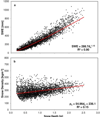
The pairwise relations between snow depth, snow density, and SWE from the historic snow course records are presented in Fig. 3. A strong correlation exists between snow depth and SWE, which is best fit as a power function (Fig. 3a). There is considerable scatter about the linear fit for snow density ver-sus snow depth (Fig. 3b), which suggests that additional vari-ables should be included to describe the variability of snow density. Snowpack relations shown here are similar to those found in previous studies (e.g., Jonas et al., 2009; Sturm et al., 2010).
SWE = 288.7ds1.15
R² = 0.90
0 200 400 600 800 1000 1200
SWE
[m
m
]
Snow Depth [m] a
ρs = 54.96ds + 236.1
R² = 0.15
0 100 200 300 400 500 600 700 800
0.0 0.5 1.0 1.5 2.0 2.5 3.0
Sno
w
Den
s
ity
[k
gm
-3]
Snow Depth [m] b
Fig. 3.Pairwise relations of SWE and snow density with snow depth from historic snow course measurements within the study area.
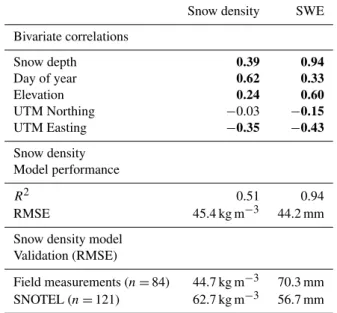
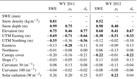
The mean snow density from the snow course data set is 287 kg m−3with a standard deviation of 64.8 kg m−3. SWE and snow depth have a greater coefficient of variation (0.65, 0.50, respectively) compared to snow density (0.23). Snow density is most highly correlated with Julian day, and also shows a positive correlation with snow depth and elevation and negative correlation with UTM Easting (Table 1). The location-dependent correlation with snow density has been shown in previous studies (e.g., Mizukami and Percia, 2008), however, is often based on a larger domain and is represen-tative of differences in climatology. The correlation of UTM Easting and snow density found from this basin scale data set may be representing the impact of the distance to a mountain barrier or storm track patterns on snow density patterns.
The final snow density model takes the following form: ρs =844+1.06DOY+26.1ds0.5
Table 1.Historic snow course bivariate correlations between snow density, SWE, snow depth, Julian day, elevation, UTM Northing, and UTM Easting and snow density model calibration and valida-tion performance statistics. Performance statistics for snow water equivalent based on using modeled snow density and observed snow depth to calculate SWE. Bolded values represent statistical signifi-cance (pvalue < 0.05).
Snow density SWE
Bivariate correlations
Snow depth 0.39 0.94
Day of year 0.62 0.33
Elevation 0.24 0.60
UTM Northing −0.03 −0.15
UTM Easting −0.35 −0.43
Snow density Model performance
R2 0.51 0.94
RMSE 45.4 kg m−3 44.2 mm
Snow density model Validation (RMSE)
Field measurements (n=84) 44.7 kg m−3 70.3 mm SNOTEL (n=121) 62.7 kg m−3 56.7 mm
model are normally distributed and do not violate the under-lying assumptions of the regression (normality, linearity, ho-moscedasticity).
The calibrated model underestimated more dense snow-packs and overestimated less dense snowsnow-packs, while calcu-lated SWE showed generally unbiased residuals that tended to slightly increase with increasing observed SWE (Fig. 4). Performance statistics calculated from the residuals of cali-bration with the original data set showed that predicted snow density explained 51 % of the total variance in the data with a RMSE of 45.4 kg m−3, yet, calculated SWE was able to ex-plain 94 % of the variance in the data and had a RMSE of 44.2 mm (Table 1).
Various methods of model evaluation were performed to test the utility of the regression model that all showed simi-lar trends (Fig. 4) and comparable error estimates (Table 1) to model calibration. As expected, a minor increase in error estimation was observed for model validation with indepen-dent data, yet the minimal increase in error shows that the regression model should be transferable to independent data within the bounds of the original data set. Thus, we used the snow density model to calculate SWE for WY 2011 and WY 2012 field-based snow depth measurements.
4.2 Basin scale SWE variability
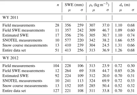
A total of 51 and 127 snowpack measurements (both opera-tional and field-based) were analyzed from the 2 April 2011
(WY 2011) and 31 March 2012 (WY 2012) snow surveys, respectively (Fig. 1). The mean SWE and snow depth from WY 2011 were greater than WY 2012, yet the mean snow density and standard deviation of snow density was shown to be consistent among both years (Table 2). The WY 2011 was the maximum snow year on record within the study area, while WY 2012 was one of the lowest snow years on record (Fig. 2); thus WY 2011 snowpack measurements were shown to have a higher mean SWE and snow depth, but also had a greater range of variability than that of WY 2012 (Table 2). From the average SWE among SNOTEL stations within the study area, the 1 April snow survey occurred before peak SWE in 2011, however, it occurred slightly after peak SWE yet before substantial melt had occurred in 2012. Analysis of the 1 April snowpack from these two water years allows for the comparison between the two extreme snow years (maxi-mum and mini(maxi-mum) as well as between two different stages of the niveograph (before and just after peak SWE).
0 200 400 600 800 1000 1200
0 200 400 600 800 1000 1200
M
o
d
e
le
d
S
W
E
[
m
m
]
Observed SWE [m m ]
Model Calibration Field Validation [R2= 0.92]
[R2= 0.94]
0 100 200 300 400 500 600
0 100 200 300 400 500 600
M
o
d
e
le
d
S
n
o
w
D
e
n
s
it
y
[
k
g
m
-3]
Observed Snow Density [kgm-3]
Model Calibration
Field Validation
[R2= 0.51]
[R2= 0.56]
Fig. 4.Snow density model versus observed snow density and SWE calibration with historic snow course data and validation with indepen-dent field data. Modeled SWE is derived from modeled snow density and observed snow depth.
Table 2.Summary statistics (µ=mean, σ=standard deviation) for snowpack properties from WY 2011 and WY 2012 snow surveys.
Statistics calculated separately for manual and operational measurements as well as manual measurements in which SWE was estimated from the snow density model.
n SWE (mm) ρs(kg m−3) ds(m)
µ σ µ σ µ σ
WY 2011
Field measurements 28 356 259 307 37.0 1.10 0.68 Field SWE measurements 11 357 242 309 46.7 1.09 0.60
Estimated SWE 17 356 276 305 30.7 1.10 0.74
SNOTEL measurements 10 577 220 342 38.2 1.66 0.55 Snow course measurements 13 410 239 304 24.5 1.31 0.66
Entire data set 51 413 256 313 36.9 1.26 0.68
WY 2012
Field measurements 104 228 106 313 23.9 0.72 0.30 Field SWE measurements 12 264 69 318 44.7 0.85 0.26
Estimated SWE 92 224 109 312 20.0 0.70 0.31
SNOTEL measurements 10 241 113 324 69.9 0.72 0.33 Snow course measurements 13 152 105 285 50.4 0.52 0.32 Entire data set 127 221 108 311 33.8 0.70 0.31
are usually on slopes less than 35◦, so steeper slopes can be underrepresented.
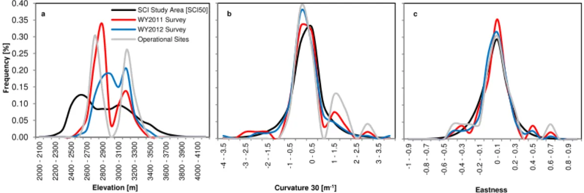
Snowpack variables were shown to have a strong correla-tion with each other, with SWE and snow depth showing the strongest relation (consistent with the historic snow course data set), while also showing to be highly correlated with elevation (Table 3). Bivariate relations showed that SWE in-creased with increasing elevation, with the steepness of this trend being greater in WY 2011 than 2012. The strength of the correlation between SWE and elevation for WY 2011 (r=0.75) and WY 2012 (r=0.68) suggests that elevation is the most important physiographic variable for driving the distribution of SWE across the study domain, which is con-sistent with previous findings from studies evaluating SWE at the basin scale (e.g., Fassnacht et al., 2003; Jost et al., 2007; Harshburger et al., 2010). As UTM Northing increases, SWE
0.00 0.05 0.10 0.15 0.20 0.25 0.30 0.35 0.40 2 0 0 0 2 1 0 0 2 2 0 0 2 3 0 0 2 4 0 0 2 5 0 0 2 6 0 0 2 7 0 0 2 8 0 0 2 9 0 0 3 0 0 0 3 1 0 0 3 2 0 0 3 3 0 0 3 4 0 0 3 5 0 0 3 6 0 0 3 7 0 0 3 8 0 0 3 9 0 0 4 0 0 0 4 1 0 0 F re qu e nc y [%] Elevation [m]
SCI Study Area [SCI50] WY2011 Survey WY2012 Survey Operational Sites a -4 -3 .5 -3 -2 .5 -2 -1 .5 -1 -0 .5 0 0 .5 1 1 .5 2 2 .5 3 3 .5
Curvature 30 [m-1] b -1 -0 .9 -0 .8 -0.7 -0 .6 -0 .5 -0 .4 -0 .3 -0 .2 -0 .1 0 0 .1 0 .2 0 .3 0 .4 0 .5 0 .6 0 .7 0 .8 0 .9 Eastness c
Fig. 5.Histograms of terrain variables across the SCI 50 study area compared to variables associated with snow measurement locations.
UTM Easting, which corresponds to both the effect of oro-graphic precipitation within the study area (the continental divide is located on the western border of the study area), and also lower elevation regions receiving less snow than higher-elevation regions. The other variables that are known to influence snow accumulation (e.g., forest cover and solar radiation) did not exhibit strong bivariate correlations with SWE, thus partial correlations were calculated to test these variables once the trends of elevation and UTM coordinates had been removed. The partial correlation is defined as the correlation between two variables, while the effect of a set of controlling variables is removed (through linear regression). Partial correlations between SWE and terrain/canopy vari-ables (with the correlation effect of elevation, UTM Easting, and UTM Northing removed) shows that curvature and slope become more important variables when the other trends are removed (Table 4).
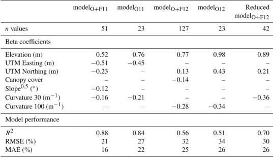
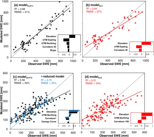
Multiple linear regression was used to model SWE for 2 April 2011 and 31 March 2012 with the operational and field-based snowpack data set (modelO+F) and the operational snowpack data set only (modelO)(Fig. 6). The final indepen-dent variables used within each model, beta coefficient val-ues, and a summary of model performance statistics is pro-vided in Table 5 and Fig. 6. To satisfy the assumptions of the regression model and improve overall model performance, a square root transformation was made to SWE (dependent variable) and slope (independent variable) for modelO+F11, which explains 88 % of the total variance with an RMSE of 85.6 mm (all RMSE values were calculated after trans-formed values have been converted back). ModelO+F12(no data transformations) explained 56 % of the total variance and showed an RMSE of 71.5 mm. The operational models were evaluated against observed values from the entire oper-ational and field data set. The WY 2011 operoper-ational model (modelO11) explains 84 % of the total variance of the data with an RMSE of 110.1 mm and includes a square root trans-formation of SWE. Lastly, modelO12 explains 51 % of the total variance with a RMSE of 75.6 mm. The VIF is less than 1.4 for each variable within all four of the multiple regres-sion models, suggesting that multicollinearity between
inde-pendent variables is not observed. Also, the residuals of each regression model do not violate the underlying assumptions of the regression (normality, linearity, homoscedasticity).
A comparison of the standardized error estimation be-tween WY 2011 and WY 2012 models shows that the modelO+F11 has a lower standardized typical magnitude of error (standardized RMSE) than modelO+F12, and describes more of the variance in the data (R2)(Table 5). Similarly, modelO11 has a lower standardized RMSE and greater R2 value than modelO12, but the difference between these two models is less (Table 5). The difference among these per-formance statistics can partially be explained by the na-ture of each snow year (WY 2011 was the maximum snow year and WY 2012 was amongst the lowest) and sampling scheme. WY 2011 showed much more variation in snow amounts than WY 2012, which could explain the difference in the RMSE. Additionally, the greater number of measure-ment locations (n=127) in WY 2012 compared to WY 2011 (n=51) could further explain the difference inR2between modelO+F11and modelO+F12. Given this difference in field-based sampling locations, a reduced modelO+Ffor WY 2012 was developed, including only WY 2012 field-based surement locations that were co-located with WY 2011 mea-surement locations (n=42). The reduced model included UTM Northing, elevation, and curvature 30 as independent variables and explained 70 % of the total variance with a stan-dardized RMSE of 30 % (Fig. 6). The reduced model shows more favorable results than the full model (modelO+F12), suggesting that fewer data points may be the reason for the stronger performance of the WY 2011 models. However, the reduced model also explained less of the variance in the data than modelO+F11, which suggests that the superior perfor-mance of the 2011 models could be due to the greater range of observed variability in the data.
5 Discussion
Table 3.Bivariate correlations between SWE, snow density, snow depth, and terrain and canopy variables for the water year 2011 and 2012 snow surveys. Bolded values represent statistical significance (pvalue < 0.05).
WY 2011 WY 2012
SWE ρs ds SWE ρs ds
SWE (mm) – – – – – –
Snow density (kg m−3) 0.81 – – 0.52 – –
Snow depth (m) 0.99 0.75 – 0.98 0.40 –
Elevation (m) 0.75 0.46 0.77 0.68 0.41 0.67
UTM Easting (m) −0.69 −0.71 −0.66 −0.38 −0.51 −0.33
UTM Northing (m) −0.55 −0.36 −0.56 −0.12 −0.02 −0.10
Eastness −0.13 −0.28 −0.11 0.10 −0.09 0.13
Northness −0.01 −0.08 0.00 0.06 −0.13 0.08
Canopy cover −0.20 −0.16 −0.21 −0.22 −0.01 −0.22
Slope (◦) −0.03 −0.05 −0.01 0.11 0.05 0.13 Curvature 30 (m−1) 0.08 0.13 0.08 −0.08 −0.11 −0.04 Curvature 100 (m−1) −0.04 −0.02 −0.02 −0.08 −0.08 −0.06 Solar radiation (W m−2) 0.26 0.20 0.25 0.07 0.22 0.04
Table 4.Partial correlations between SWE and terrain/canopy vari-ables with the effect of elevation (z), UTM Easting (x), and UTM Northing (y) removed. Bolded values represent statistical signifi-cance (pvalue < 0.05).
WY 2011 WY 2012
z z, x, y z z, x, y
UTM Easting (m) −0.74 – −0.16 –
UTM Northing (m) −0.38 – 0.16 –
Eastness −0.07 0.23 0.08 0.10
Northness 0.06 0.18 0.12 0.16
Canopy cover −0.14 0.06 −0.15 −0.17 Slope (◦) −0.22 −0.28 −0.08 −0.06 Curvature 30 (m−1) −0.07 −0.41 −0.32 −0.31 Curvature 100 (m−1) −0.25 −0.31 −0.36 −0.35 Solar radiation (W m−2) 0.02 −0.10 −0.06 −0.13
snow depth measurements. Predicted SWE RMSE ranged from 44 mm (calibration data) to 70 mm (independent field validation data). Eighty percent of all residual values (n=2613) fell within ±50 mm, and the variance of the model residuals was on average within 12.8 % of the ob-served values for the calibration data set. Within site vari-ability of SWE has been conservatively estimated to be 15 to 25 % (Jonas et al., 2009), which suggests that the error ob-served from the model is within the natural range of SWE variability at a site (Fassnacht et al., 2008). The small range of error suggests that estimating SWE from snow depth mea-surements through a snow density model works due to the conservative nature of snow density; 52 % of snow density data values ranged from 250 to 350 kg m−3.
Using historical operational measurements for develop-ment of a basin scale snow density model has implications for future field-based basin scale sampling campaigns,
sug-gesting a sampling scheme dominated by snow depth mea-surements may be successful for evaluating basin scale SWE variability. The strength and utility of the model developed here is its ability to estimate SWE from the most easily mea-sured variable, snow depth. Across basin scales, efforts are being made to estimate snow depth using both airborne li-dar and satellite-based lili-dar data, such as ICESat (Jasinski et al., 2012). Snow density models will be especially useful for these applications. The utility of a snow density model is also very valuable for field-based snow surveys at the basin scale, in which many snowpack measurements are required, and the assumption of a constant snow density across the study area is not valid (Lopéz-Moreno et al., 2013).
The snow density model is simple to develop and imple-ment and is an effective tool for obtaining estimates of SWE from snow depth measurements across basin scale domains. The model is, however, constricted to its spatial domain, range of physiographic inputs, as well as temporal coverage, thus it may not be applicable to areas outside of the study area for elevations that are lower than 2408 m or higher than 3261 m, or for snow depths shallower than 0.20 m or deeper than 2.52 m.
Table 5.Beta coefficients (standardized coefficients) and performance statistics for each multiple regression model with dependent variable SWE (mm). Each coefficient included in the models was statistically significant (pvalue < 0.05). Model performance metrics are evaluated against the entire data set (both operational and field) for each year. RMSE and MAE statistics are reported as standardized values (value of the statistic divided by the mean of the observations).
modelO+F11 modelO11 modelO+F12 modelO12 Reduced modelO+F12
nvalues 51 23 127 23 42
Beta coefficients
Elevation (m) 0.52 0.76 0.77 0.98 0.89
UTM Easting (m) −0.51 −0.45 – – –
UTM Northing (m) −0.23 – 0.13 0.43 0.21
Canopy cover – – −0.14 – –
Slope0.5(◦) −0.12 – – – –
Curvature 30 (m−1) −0.16 −0.21 – – −0.36
Curvature 100 (m−1) – – −0.28 −0.34 –
Model performance
R2 0.88 0.84 0.56 0.51 0.70
RMSE (%) 21 27 32 34 30
MAE (%) 16 22 25 26 26
that are orders of magnitude larger than what has been pre-sented here, with the current data being at a finer resolution. We have applied the snow density alpine model developed by Sturm et al. (2010) to our data set and directly compared the results to those of our snow density model, given their model was developed for global applications and data from the western US were used within model development. We did not, however, test the model developed by Jonas et al. (2009), as it was developed specifically for Switzerland and requires regional and elevational parameters that are specific to this area, and was not developed for use in other areas. The Sturm et al. (2010) alpine model performed well when applied to the data set from this study, showing a snow density RMSE of 58.1 kg m−3and RMSE of 53.4 mm when used to calcu-late SWE. Also, the variance described in the SWE data set from this study by the Sturm et al. (2010) model showed a similarly strong performance (R2=0.91) as our model. However, the model developed in this study outperformed the Sturm et al. (2010) model, showing an improvement in RMSE for snow density and SWE by 22 % and 17 %, re-spectively. Also, our model showed an improvement of field validation RMSE by 9 % for snow density and 7 % for SWE. This shows that calibrating a snow density model to a spe-cific basin of interest can improve estimates of SWE from snow depth from models developed from larger domains and should be considered for future basin scale assessments of SWE.
Despite WY 2011 being a maximum snow year and WY 2012 being a minimum snow year, the variables driving each SWE regression were similar and included elevation, loca-tion within the basin (UTM Easting and/or UTM Northing),
0 200 400 600 800 1000
0 200 400 600 800 1000
M
odel
e
d
S
W
E
[
m
m
]
Observed SWE [mm]
R2 = 0.88 RMSE = 21%
[a] modelO+F11
0 200 400 600 800 1000
Observed SWE [mm]
R2 = 0.84
RMSE = 27%
[b] modelO11
0 100 200 300 400 500 600
0 100 200 300 400 500 600
M
odel
e
d
S
W
E
[
m
m
]
Observed SWE [mm] reduced model
R2 = 0.56 RMSE = 32%
[c] modelO+F12
R2 = 0.70 RMSE = 30%
0 100 200 300 400 500 600
Observed SWE [mm]
R2 = 0.51
RMSE = 34%
[d] modelO12
-1 -0.5 0 0.5 1
Slope Curvature 30 UTM Northing UTM Easting Elevation
-1 -0.5 0 0.5 1
Curvature 30 UTM Easting Elevation
-1 -0.5 0 0.5 1
Canopy Cover Curvature* UTM Northing Elevation
-1 -0.5 0 0.5 1
Curvature 100 UTM Northing Elevation
Fig. 6.Scatterplots showing observed versus modeled SWE from modelO+F (shown in black) and modelO (shown in red) for both WY
2011 and 2012. The observed values used to evaluate each model include the combined operational and field-based data set. The reduced modelO+F12includes only field-based measurement locations also sampled during WY 2011 (shown in blue). The callout bar graphs show the relative influence of each model coefficient (beta coefficients). Curvature* represents curvature 100 for modelO+F12and curvature 30 for the reduced model.
take into the account shading from tree canopy, therefore it is not representative of solar radiation across the basin scale. Additionally, although the canopy cover variable did show the negative correlation with SWE as expected, this correla-tion was relatively weak, thus the categorical canopy cover variable we use here is likely not adequate. There is a need for a finer resolution canopy data set for basin scale anal-yses, as the 30 m-resolution National Land Cover Database (NLCD 2001) canopy density data are not adequate; this data set often shows SNOTEL stations as having high canopy den-sity values despite their location within small forest open-ings. Future basin scale snow studies should focus on in-corporating a more accurate representation of the influence of forest canopy and solar radiation on snowpack variability (Musselman et al., 2013). Given that studies (e.g., Fassnacht et al., 2012) have shown the spatial variability of snow ac-cumulation to be described by different physiographic vari-ables from year to year, additional years of data collection at the basin scale are needed for a more complete evaluation of the drivers of SWE distribution.
Comparison of the error between modelO+F and modelO for WY 2011 and WY 2012 shows that modelO+F has
superior performance statistics for both years (Table 5). ModelO+F showed a 22 % and 5 % improvement in RMSE from modelO in 2011 and 2012, respectively. However, modelO11and modelO12showed a fairly strong performance with similar predictor variables as the operational plus field models. The operational regression models may not be repre-senting the study area, as SNOTEL measurements have been shown to represent point locations rather than surrounding areas (Molotch and Bales, 2005) often having more snow (Daly et al., 2000), and tend to be located in areas with sim-ilar physiographic features (flat and open canopy areas lo-cated near tree line).
● ● ● ● ● ● ● ● ● ● ● ● ● ● ● ● ● ● ● ● ● ● ● ● ● ●●● ● ● ● ● ● ● ● ● ● ● ● ● ● ● ● ● ● ● ● ● ● ● ● WY 2011 4470000 4480000 4490000 4500000 4510000 4520000
420000 430000 440000 450000 UTM Easting UTM Nor thing 0 200 400 600 800 SWE [mm] ● ● ● ● ● ● ● ● ● ● ● ● ● ● ● ● ● ● ● ● ●● ● ● ● ● ● ● ● ● ● ● ● ● ● ● ● ● ● ● ●●● ● ● ● ● ● ● ● ● ● ● ● ● ● ● ●●●●● ●●●●●●●● ●●●●●●●● ● ●●●●●●●● ● ● ● ● ● ● ● ● ● ● ● ● ● ● ●●● ● ● ● ● ● ● ● ● ● ● ● ● ● ● ● ● ● ● ● ● ● ● ● WY 2012 4470000 4480000 4490000 4500000 4510000 4520000
420000 430000 440000 450000 UTM Easting UTM Nor thing 0 100 200 300 400 500 SWE [mm]
Fig. 7.SWE plotted against UTM Northing and UTM Easting for both WY 2011 and WY2012 snow surveys.
model. The comparisons of the statistical relation of the snowpack with terrain-based variables and physically based snow evolution modeling can provide insight for basin scale SWE distribution estimations.
There are limitations to this study that must be acknowl-edged. The representivity of snow measurements of their sur-roundings is an important issue often raised in snow hydrol-ogy studies (e.g., Molotch and Bales, 2005). Although our field-based measurements attempted to account for the fine-scale variability by taking 11 measurement points at each sampling location, it is possible these sampling locations could have fallen on the edge of a 30 m-resolution GIS pixel and not accurately sampled associated terrain variables. The SNOTEL station snow pillows have been shown to not rep-resent their surroundings, which could have caused further inaccuracies of the DEM-derived variables at each of these sites. The use of multiple linear regression to model non-linear processes for the SWE models developed within this study is another important limitation. Limitations in this ap-proach have been presented in previous studies (Elder et al., 1995), however, we do believe that multiple linear regression was appropriate given the goals of our study. We would have ideally used binary regression trees (e.g., Elder et al., 1998) to develop the SWE models, but these decision tree models require larger datasets than available in this study to provide meaningful results. Given the main goal of the SWE models was used as a tool to evaluate the importance of individual variables rather than used strictly within a predictive frame-work, the multiple linear regression models provide simplic-ity of the interpretation of model coefficients. Finally, our field sampling strategy (non-uniform, non-random spacing, and clustered pattern), which is a different spacing than op-erational data, may have influenced regression results. Given the extent of the study area evaluated (1493 km2), it was
nec-essary to employ this transect-based strategy because of the formidable challenge of accessing these areas throughout the basin on skis. Each sampling transect with 500 m spacing of sampling locations were generally around four kilometers in length and located along an elevational gradient with varying terrain, providing a range of snow conditions to be sampled (Fig. 1). Further evaluation of each of the individual sam-pling clusters (Colorado State University Pingree Park Cam-pus, Cameron Pass, and Deadman Hill) showed that eleva-tion and locaeleva-tion have the strongest correlaeleva-tion with SWE, suggesting the 500 m spacing of the field-based sampling lo-cations is likely large enough to represent our scale of in-terest. A plot of UTM Easting and UTM Northing versus SWE (Fig. 7) shows clear regional trends of the distribution of SWE across the study area. The importance of the UTM coordinates in describing the SWE distribution is likely not being affected by the sampling clusters, as these same trends were observed from the operational data (modelO). Future snow field campaigns at the basin scale should take strong consideration of the best sampling strategy suited for the challenges of covering the basin scale.
6 Conclusions
We have used a combination of operational and field-based snow measurements to evaluate snowpack properties across the basin scale. This research was motivated by the need for additional ground-truth snowpack observations at a scale that coincides with that of remote sensing observations and is es-pecially pertinent to water resources forecasting.
independent variables of snow depth, day of year, elevation, and UTM Easting were used in a multiple linear regression model to estimate snow density. Statistics showed strong per-formance of SWE calculated from snow depth observations using the snow density model, and model validation sug-gests the model is transferable to independent data within the bounds of the original data set. The methods here provide a pathway for estimating SWE from snow depth measure-ments, which is especially useful when evaluating snowpack properties at the basin scale, where time-consuming field-based measurements of SWE are often not feasible.
The spatial variability of SWE within the Cache la Poudre Basin was analyzed using operational and field-based snow-pack measurements from WY 2011 and WY 2012. Bivari-ate and partial correlations of SWE with terrain and canopy variables as well as multiple linear regression models show that elevation, UTM Easting, UTM Northing, and curvature are most highly correlated with SWE during both years, and thus likely are explanatory variables describing processes that drive spatial variability at this scale (e.g., orographic pre-cipitation, synoptic weather patterns, and wind redistribution of snow). Solar radiation is also likely one of the main drivers of basin scale snow variability, however this variable was nei-ther adequately sampled nor modeled in this study, suggest-ing its lack of significance may have been a misrepresentative statistical finding.
The continuity of field-based snowpack measurements, as provided within this study, is essential given the assump-tion of non-staassump-tionarity from hydroclimatic change (Milly et al., 2008) and indications of more extreme conditions (IPCC, 2007). This examination of two very different snow years may represent the bounds of extremes and possibly the limitations due to non-stationarity. Continued field measure-ments of the snowpack will aid advancement of remote sens-ing and modelsens-ing applications, but more importantly con-tinue to provide ground-truth observations for evaluating the complexities and uncertainties of the changing earth system.
Acknowledgements. This research was supported by the NASA Terrestrial Hydrology Program (Grant #NNX11AQ66G, Principal Investigator M. F. Jasinski, NASA-GSFC). Support for publishing was provided from the Colorado State University Libraries Open Access Research and Scholarship Fund. Thanks to J. Meiman for discussions on basin scale snow variability. We acknowledge the contributions of the Natural Resources Conservation Service for the collection of SNOTEL and snow course measurements. Those who helped with field data collection are acknowledged with thanks. We would like to thank A. Winstral of ARS and an anonymous review for their constructive comments.
Edited by: D. Hall
References
Akaike, H.: A new look at the statistical model identification, IEEE T. Automat. Contr., 19, 716–723, 1974.
Anderton, S. P., White, S. M, and Alvera, B.: Evaluation of spatial variability in snow water equivalent for a high mountain catch-ment, Hydrol. Process., 18, 435–453, 2004.
Bales, R. C., Molotch, N. P., Painter, T. H., Dettinger, M. D., Rice R., and Dozier, J.: Mountain hydrology of the western United States, Water Resour. Res., 42, W08432, doi:10.1029/2005WR004387, 2006.
Balk, B. and Elder, K.: Combining binary decision tree and geo-statistical methods to estimate snow distribution in a mountain watershed, Water Resour. Res., 36, 13–26, 2000.
Barry, R. G.: Mountain Weather and Climate, 3rd Edn., Cambridge University Press, Cambridge, 2008.
Berk, K. N.: Comparing Subset Regression Procedures, Technomet-rics, 20, 1–6, 1978.
Blöschl, G.: Scaling issues in snow hydrology, Hydrol. Process., 13, 2149–2175, 1999.
Blöschl, G., Kirnbauer, R., and Gutknecht D.: Distributed Snowmelt Simulations in an Alpine Catchment 1. Model Evaluation on the Basis of Snow Cover Patterns, Water Resour. Res., 27, 3171– 3179, 1991.
Clow, D. W.: Changes in the Timing of Snowmelt and Streamflow in Colorado: A Response to Recent Warming, J. Climate, 23, 2293– 2306, 2010.
Daly, S. F., Davis, R., Ochs, E., and Pangburn, T.: An approach to spatially distributed snow modeling of the Sacramento and San Joaquin basins, California, Hydrol. Process., 14, 3257–3271, 2000.
Dingman, S. L.: Elevation: A major influence on the hydrology of New Hampshire and Vermont, USA, Hydrol. Sci. Bull., 26, 399– 413, 1981.
Doesken, N. J. and Judson, A.: The Snow Booklet: A Guide to the Science, Climatology, and Measurement of Snow in the United States, Dep. of Atmos. Sci., Colorado State Univ., Fort Collins, CO, 1996.
Dressler, K., Fassnacht, S. R., and Bales, R. C.: A Comparison of Snow Telemetry and Snow Course Measurements in the Col-orado River Basin, J. Hydrometeorol., 7, 705–712, 2006. Elder, K., Dozier, J., and Michaelson, J.: Snow accumulation and
distribution in an Alpine watershed, Water Resour. Res., 27, 1541–1552, 1991.
Elder, K., Michaelsen, J., and Dozer, J.: Small basin modelling of snow water equivalence using binary regression tree methods, Proc. Symp. on Biogeochemistry of Seasonally Snow-Covered Catchments, Boulder, CO, IAHS-AIHS and IUGG XX General Assembly, IAHS Publication 228, 129–139, 1995.
Elder, K., Rosenthal, W., and Davis, R. E.: Estimating the spatial distribution of snow water equivalence in a montane watershed, Hydrol. Process., 12, 1793–1808, 1998.
Erickson, T. A., Williams, M. W., and Winstral, A.: Persistence of topographic controls on the spatial distribution of snow in rugged mountain terrain, Colorado, United States, Water Resour. Res., 41, W04014, doi:10.1029/2003WR002973, 2005.
ESRI: ArcGIS Desktop: Release 10. Redlands, CA: Environmental Systems Research Institute, 2011.
River Basin, Proceedings of 58th Eastern Snow Conference, Ot-tawa, Ontario, Canada, May 2001.
Fassnacht, S. R., Dressler, K. A., and Bales, R. C.: Snow water equivalent interpolation for the Colorado River Basin from snow telemetry (SNOTEL) data, Water Resour. Res., 39, 1208–1218, 2003.
Fassnacht, S. R., Skordahl, M. E., and Derry, J. E.: Variability at Colorado Operational Snow Measurement Sites, Snowcourse Stations at Collocated Snow Telemetry Stations, Proceedings of 65th Eastern Snow Conference, Fairlee, Vermont, USA, May 2008.
Fassnacht, S. R., Heun, C. M., López-Moreno, J. I., and Latron, J. B. P.: Variability of Snow Density Measurements in the Rio Esera Valley, Pyrenees Mountains, Spain, Cuandernos de Investigación Geográfica J. Geogr. Res., 36, 59–72, 2010.
Fassnacht, S. R., Dressler, K. A., Hulstrand, D. M., Bales, R. C., and Patterson, G.: Temporal Inconsistencies in Coarse-Scale Snow Water Equivalent Patterns: Colorado River Basin Snow Telemetry-Topography Regressions, Pirineos, 167, 167– 186, 2012.
Harshburger, B. J., Humes, K. S., Walden, V. P., Blandford, T. R., Moore, B. C., and Dezzani, R. J.: Spatial interpolation of snow water equivalency using surface observations and remotely sensed images of snow-covered area, Hydrol. Process., 24, 1285– 1295, 2010.
Intergovernmental Panel on Climate Change (IPCC): Climate Change 2007: The Physical Science Basis: Contribution of Working Group I to the Fourth Assessment Report of the IPCC, edited by: Solomon, S., Qin, D., Manning, M., Chen, Z., Mar-quis, M., Averyt, K. B., Tignor, M., and Miller, H. L., Cambridge Univ. Press, Cambridge, UK, 2007.
Jasinski, M., Stoll, J., Carabajal, C., and Harding, D.: Feasibility of Estimating Snow Depth in Complex Terrain Using Satellite Lidar Altimetry, Eastern Snow Conference, Claryville, NY, 5–12 June 2012, 2012.
Jepsen, S. M., Moltch, N. P., Williams, M. W., Rittger, K. E., and Sickman, J. O.: Interannual variability of snowmelt in the Sierra Nevada and Rocky Mountains, United States: Examples from two alpine watersheds, Water Resour. Res., 48, W02529, doi:10.1029/2011WR011006, 2012.
Jonas, T., Marty, C., and Magnusson, J.: Estimating the snow water equivalent from snow depth measurements in the Swiss Alps, J. Hydrol., 378, 161–167, 2009.
Jost, G., Weiler, M., Gluns, D. R., and Alila, Y.: The influence of forest and topography on snow accumulation and melt at the watershed-scale, J. Hydrol., 347, 101–115, 2007.
Kerr, T., Clark, M., Hendrikx, J., and Anderson, B.: Snow distri-bution in a steep mid-latitude alpine catchment, Adv. Water Re-sour., 55, 17–24, 2013.
Kimerling, A. J., Buckley, A. R., Muehrcke, P. C., and Muehrcke, J. E.: Map Use: Reading Analysis Interpretation, Seventh Edition, ESRI Press Academic, Redlands, California, 2011.
Kutner, M. H., Nachtsheim, C. J., Neter, J., and Li, W.: Applied Lin-ear Statistical Models, Fifth Edition. McGraw-Hill/Irwin, New York, NY, 2005.
Lapen, D. R. and Martz, L. W.: An investigation of the spatial as-sociation between snow depth and topography in a prairie agri-cultural landscape using digital terrain analysis, J. Hydrol., 184, 277–298, 1996.
Liston, G. E. and Sturm, M.: A snow-transport model for complex terrain, J. Glaciol., 44, 498–516, 1998.
Logan, L. A.: Basin-wide water equivalent estimation from snow-pack depth measurements, IAHS-AISH P., 107, 864–884, 1973. López-Moreno, J. I. and Nogués-Bravo, D.: Interpolating local
snow depth data: an evaluation of methods, Hydrol. Process., 20, 2217–2231, 2006.
López-Moreno, J. I., Fassnacht, S. R., Beguería, S., and Latron, J. B. P.: Variability of snow depth at the plot scale: implications for mean depth estimation and sampling strategies, The Cryosphere, 5, 617–629, doi:10.5194/tc-5-617-2011, 2011.
López-Moreno, J. I., Fassnacht, S. R., Heath, J. T., Musselman, K. N., Revuelto, J., Latron, J., Morán-Tejeda, E., and Jonas, T.: Small scale spatial variability of snow density and depth over complex alpine terrain: Implications for estimating snow water equivalent, Adv. Water Resour., 55, 40–52, 2013.
Mallows, C. L.: Some Comments onCp, Technometrics, 15, 661– 675, 1973.
McClung, D. and Schaerer, P.: The Avalanche Handbook, Third Edition, The Mountaineers Books, Seattle, WA, 2006.
Milly P. C. D., Betancourt, J., Falkenmark, M., Hirsch, R. M., Zbig-niew, W. K., Lettenmaier., D. P., and Stouffer, R. J.: Stationarity Is Dead: Whither Water Management?, Science, 319, 573–574, 2008.
Mizukami, N. and Perica, S.: Spatiotemporal characteristics of snowpack density in the mountainous regions of the Western United States, J. Hydrometeorol., 9, 1416–1426, 2008.
Molotch, N. P. and Bales, R. C.: Scaling snow observations from the point to the grid element: Implications for ob-servation network design, Water Resour. Res., 41, W11421, doi:10.1029/2005WR004229, 2005.
Molotch, N. P., Colee, M. T., Bales, R. C., and Dozier, J.: Estimat-ing the spatial distribution of snow water equivalent in an alpine basin using binary regression tree models: The impact of digital elevation data and independent variable selection, Hydrol. Pro-cess., 19, 1459–1479, 2005.
Montesi, J., Elder, K., Schmidt, R. A., and Davis, R. E.: Sublimation of Intercepted Snow within a Subalpine Forest Canopy at Two Elevations, J. Hydrometeorol., 5, 763–773, 2004.
Musselman, K. N., Margulis, S. A., and Molotch, N. P.: Estimation of solar direct beam transmittance of conifer canopies from air-borne LiDAR, Remote Sens. Environ., 136, 402–415, 2013. Pomeroy, J. W. and Gray, D. M.: Snow Accumulation, Relocation
and Management. National Hydrology Research Institute Sci-ence Report No. 7, 1995.
R Development Core Team: R: A language and environment for statistical computing. R Foundation for Statistical Computing, Vievva, Austria, ISBN 3-900051-07-0, http://www.R-project. org/, 2012.
Richer, E. E., Kampf, S. K., Fassnacht, S. R., and Moore, C. C.: Spatiotemporal index for analyzing controls on snow climatol-ogy: Application in the Colorado Front Range, Phys. Geogr., 34, 85–107, doi:10.1080/02723646.2013.787578, 2013.
Stewart, I. T.: Changes in snowpack and snowmelt runoff for key mountain regions, Hydrol. Process., 23, 78–94, 2009.
Viviroli, D., Weingartner, R., and Messerli, B.: Assessing the Hy-drological Significance of the World’s Mountains, Mt. Res. Dev., 23, 32–40, 2003.
Viviroli, D., Archer, D. R., Buytaert, W., Fowler, H. J., Greenwood, G. B., Hamlet, A. F., Huang, Y., Koboltschnig, G., Litaor, M. I., López-Moreno, J. I., Lorentz, S., Schädler, B., Schreier, H., Schwaiger, K., Vuille, M., and Woods, R.: Climate change and mountain water resources: overview and recommendations for research, management and policy, Hydrol. Earth Syst. Sci., 15, 471–504, doi:10.5194/hess-15-471-2011, 2011.
Veatch, W., Brooks, P. D., Gustafson, J. R., and Molotch, N. P.: Quantifying the effects of forest canopy cover on net snow ac-cumulation at a continental, mid-latitude site, Ecohydrology, 2, 115–128, 2009.
Washichak J. N. and McAndrew, D. W.: Snow Measurement Accu-racy in High Density Snow Course Network in Colorado, Pro-ceedings of the 35th Western Snow Conference, Boise, Idaho, USA, April, 1967.