Greenland accumulation and its connection to the large-scale atmospheric circulation in ERA-Interim and paleoclimate simulations

(1)

Clim. Past, 9, 2433–2450, 2013 www.clim-past.net/9/2433/2013/ doi:10.5194/cp-9-2433-2013

Climate

of the Past

Open Access

Greenland accumulation and its connection to the large-scale

atmospheric circulation in ERA-Interim and paleoclimate

simulations

N. Merz1,2,*, C. C. Raible1,2, H. Fischer1,2, V. Varma3, M. Prange3, and T. F. Stocker1,2 1_{Climate and Environmental Physics, University of Bern, Bern, Switzerland}

2_{Oeschger Centre for Climate Change Research, University of Bern, Bern, Switzerland}

3_{MARUM – Center for Marine Environmental Sciences and Faculty of Geosciences, University of Bremen,} Bremen, Germany

*_{Invited contribution by N. Merz, recipient of the EGU Outstanding Student Poster Awards 2011.}

Correspondence to:N. Merz (merz@climate.unibe.ch)

Received: 13 June 2013 – Published in Clim. Past Discuss.: 9 July 2013

Revised: 23 September 2013 – Accepted: 4 October 2013 – Published: 4 November 2013

Abstract.Changes in Greenland accumulation and the sta-bility in the relationship between accumulation variasta-bility and large-scale circulation are assessed by performing time-slice simulations for the present day, the preindustrial era, the early Holocene, and the Last Glacial Maximum (LGM) with a comprehensive climate model. The stability issue is an important prerequisite for reconstructions of Northern Hemi-sphere atmospheric circulation variability based on accu-mulation or precipitation proxy records from Greenland ice cores. The analysis reveals that the relationship between ac-cumulation variability and large-scale circulation undergoes a significant seasonal cycle. As the contributions of the indi-vidual seasons to the annual signal change, annual mean ac-cumulation variability is not necessarily related to the same atmospheric circulation patterns during the different climate states. Interestingly, within a season, local Greenland accu-mulation variability is indeed linked to a consistent circu-lation pattern, which is observed for all studied climate peri-ods, even for the LGM. Hence, it would be possible to deduce a reliable reconstruction of seasonal atmospheric variability (e.g., for North Atlantic winters) if an accumulation or pre-cipitation proxy were available that resolves single seasons. We further show that the simulated impacts of orbital forcing and changes in the ice sheet topography on Greenland accu-mulation exhibit strong spatial differences, emphasizing that accumulation records from different ice core sites regard-ing both interannual and long-term (centennial to millennial)

variability cannot be expected to look alike since they include a distinct local signature. The only uniform signal to exter-nal forcing is the strong decrease in Greenland accumulation during glacial (LGM) conditions and an increase associated with the recent rise in greenhouse gas concentrations.

1 Introduction

(2)

accumulation variability is largely attributed to changes in atmospheric circulation rather than to thermodynamic con-trol (Kapsner et al., 1995; Cruger et al., 2004; Hutterli et al., 2007). Based on this, a number of studies identify specific features of the atmospheric circulation that have an imprint on Greenland accumulation variability: Rogers et al. (2004) showed that increased cyclone activity in the proximity of the accumulation location causes anomalous high accumula-tion and that cyclone frequency variaaccumula-tions are significantly related to the primary modes of Greenland accumulation.

In some studies, the reverse approach is used to reconstruct features of atmospheric circulation from Greenland accumu-lation variability: Appenzeller et al. (1998) reconstructed the North Atlantic Oscillation (NAO) for several centuries from the NASA-U ice core. However, the agreement among vari-ous preinstrumental NAO reconstructions including NASA-U is not significant (Luterbacher et al., 2001; Pinto and Raible, 2012). A possible explanation for these diverging re-sults is the fact that the centers of action of the NAO are not stationary over time (Raible et al., 2006), resulting in a different imprint on the proxy records (Lehner et al., 2012). To avoid the uncertainties arising from the instabilities in at-mospheric modes, Hutterli et al. (2005) have linked interan-nual accumulation variability in different Greenland regions to distinct large-scale atmospheric patterns based on ERA-40 reanalysis data. The significant relationship found offers the potential to reconstruct the occurrence of these circulation patterns from ice-coderived accumulation records in re-spective regions. However, an important prerequisite for such reconstructions is the stability of the connection between lo-cal accumulation rate at the ice core site and the respective circulation pattern throughout the time of reconstruction. As seen for the NAO reconstruction (Lehner et al., 2012), this requirement is not necessarily fulfilled.

In this study we address this stability issue and use a state-of-art climate model as a test bed to revisit the rela-tionship between local accumulation and these atmospheric circulation patterns, similar to Hutterli et al. (2005). We per-form time-slice simulations for the present day, the preindus-trial era, the early Holocene and the Last Glacial Maximum (LGM) to cover a variety of past climate states. Besides the stability issue, which is of great value for the proxy inter-pretation, we use the model to investigate the influence of orbital forcing and moderate changes in the GrIS topogra-phy on the GrIS mean accumulation. The sensitivity to to-pographic changes is studied with a set of simulations that implement reconstructed ice sheet topographies from Peltier (2004) for the early Holocene. Moreover, we study in detail the relationship of local GrIS accumulation and atmospheric circulation variability, as we observe distinct seasonal fea-tures that have not been depicted in the studies using annual mean accumulation. Previous studies assessing the relation-ship between accumulation and atmospheric circulation in a paleoclimate context have focused on the LGM (Pausata et al., 2009; Langen and Vinther, 2009) in order to identify

glacial–interglacial differences. With this study we expand the discussion of the stability of these relationships to the early Holocene, a period not as different from present day as the LGM but still including distinct anomalies in solar inso-lation and the Northern Hemisphere (NH) ice sheets.

The manuscript is structured as follows: Sect. 2 describes the observational data, the model, and the experiments and includes a short description of the statistical analysis tools. In Sect. 3 we present the model results regarding Greenland accumulation during different climate states and investigate the influence of the external forcing on total and local GrIS accumulation. Section 4 focuses on the relationship between local GrIS accumulation/precipitation and the prevailing at-mospheric circulation patterns on various timescales (daily to annual). Moreover, tests on the stability of the deduced at-mospheric circulation patterns in the different time-slice sim-ulations are presented. All results are discussed in Sect. 5 and conclusions are presented in Sect. 6.

2 Data and method

2.1 Reanalysis data

The atmospheric reanalysis data set used in this study is the ERA-Interim (ERAi) product from the European Cen-tre for Medium-Range Weather Forecasts (ECMWF; Dee et al., 2011). ERAi data are originally calculated with T255 (∼80 km) resolution and available on the regular 1◦_×₁◦

grid. We use both monthly and daily data for the period of 1979–2011. Note that the daily mean surface flux fields – i.e., snowfall, total precipitation, and sublimation (also re-ferred to as snow evaporation) – are calculated as the 0 to 36 h accumulation forecast minus the 0 to 12 h accumulation forecast to avoid known spin-up effects (Uppala et al., 2005; Dee et al., 2011). In addition to ERAi, all analyses are carried out with ERA40 data (1958–2001). However, the ERA40 re-sults are very similar to ERAi. Thus, only ERAi rere-sults are presented here.

2.2 Climate model

Besides the reanalysis data, the study is based on simu-lations with the Community Climate System Model (ver-sion 4, CCSM4) developed at the National Center for At-mospheric Research (NCAR) with a horizontal resolution of 0.9◦_×_1.25◦_{(Gent et al., 2011). The model includes}

(3)

N. Merz et al.: Greenland accumulation links to atmospheric circulation 2435

Fig. 1.Paleotopographies implemented in the model simulations: deviation from present-day mask [m] for(a)7 ka,(b)8 ka,(c)9 ka, and

(d)LGM (21 ka). All topographies are based on output from the ICE-5G model by Peltier (2004).

its thermodynamic-only mode. This means that sea ice con-centration fields are prescribed and sea ice thickness is fixed (e.g., to two meters in NH) but surface fluxes are computed taking into account snow depth, albedo, and surface temper-ature over the ice using one-dimensional thermodynamics. This atmosphere–land-only setup is very cost efficient com-pared to fully coupled runs and allows us to perform a set of time-slice simulations with a fairly high horizontal resolu-tion. As a drawback, possible feedbacks with the ocean and sea ice component are excluded.

2.3 Experiments

To study the accumulation and the associated atmospheric circulation on Greenland during different recent climate states, a set of time-slice experiments is conducted covering four different time periods:

– A present-day (PD) simulation with perpetual 1990 AD condition, which is mainly used for model evaluation by comparing with reanalysis data.

– A preindustrial (PI) simulation with perpetual 1750 AD conditions used as a reference simulation for the paleosimulations since it describes the present climate without perturbation by human activities.

– Four early Holocene (EH) simulations with perpet-ual 8 ka (8000 yr before 1950) conditions but different ice sheet forcings (see Fig. 1 and Sect. 2.4 for more details).

– A Last Glacial Maximum (LGM) simulation with full glacial conditions including major ice sheets (see Fig. 1d). This simulation has previously been used and described by Hofer et al. (2012a, b).

The set of EH simulations is used to test the sensitivity of an interglacial climate to moderate changes in the ice sheet dis-tribution. These sensitivity experiments are also the reason why the Holocene experiments are placed within the early Holocene (8 ka) instead of the classical mid-Holocene (6 ka) setup as used in the Paleoclimate Modelling Intercomparison Project (PMIP) protocol (Braconnot et al., 2007). During the early Holocene, level estimates show a considerable sea-level rise resulting from significant changes in the size of the ice sheets (see Smith et al., 2011 and references therein). For 8 ka (Fig. 1b) the anomalies with respect to the present-day topography are similar to 7 ka but stronger. A list of all sim-ulations and the external forcing factors used is provided in Table 1. All simulations are conducted for 33 model years, and the analysis is based on the last 30 yr of each simulation as the first 3 yr are declared as spin-up phase.

2.4 Boundary conditions

(4)

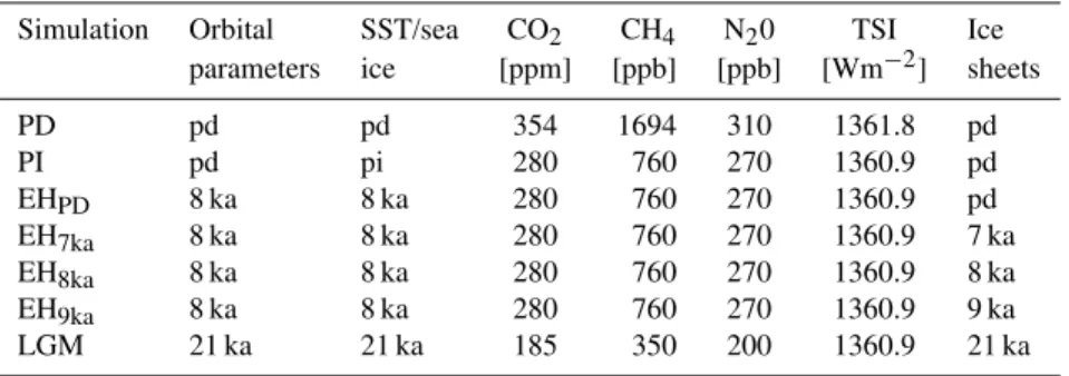
Table 1.List of model simulations and the forcing used in the experiments. Present-day levels are denoted as pd, and preindustrial levels as pi. The orbital parameters are calculated according to Berger (1978). SST and sea ice fields are outputs of corresponding fully coupled CCSM3 simulations (see Sect. 2.4 for details). The preindustrial and the LGM levels of the GHGs are following the PMIP protocol. Solar forcing is expressed as total solar irradiance (TSI), and all the values correspond to CCSM4 standard levels. The pd ice sheets are CCSM4 standard, whereas all paleo-ice sheets correspond to ICE-5G masks by Peltier (2004) as illustrated in Fig 1.

Simulation Orbital SST/sea CO₂ CH₄ N₂0 TSI Ice

parameters ice [ppm] [ppb] [ppb] [Wm−2] sheets

PD pd pd 354 1694 310 1361.8 pd

PI pd pi 280 760 270 1360.9 pd

EHPD 8 ka 8 ka 280 760 270 1360.9 pd

EH7ka 8 ka 8 ka 280 760 270 1360.9 7 ka

EH8ka 8 ka 8 ka 280 760 270 1360.9 8 ka

EH9ka 8 ka 8 ka 280 760 270 1360.9 9 ka

LGM 21 ka 21 ka 185 350 200 1360.9 21 ka

simulations we take 33 yr output of around 8 ka from a tran-sient Holocene simulation. This trantran-sient Holocene simula-tion starts at 9 ka and is similar to the CCSM3 run by Varma et al. (2012) except that no orbital acceleration is applied. For all time-slice simulations, the monthly mean SST and sea ice output of the corresponding CCSM3 simulations are used as time-varying lower boundary conditions. With this setup we account for both the different states of the ocean and sea ice cover during the different climate periods as well as for in-terannual variability in the SSTs and sea ice concentration.

The values for the Earth’s orbital parameters are calcu-lated according to Berger (1978). The influence of the or-bital forcing difference between present day and the prein-dustrial era is negligible. Similar to the mid-Holocene (e.g., Braconnot et al., 2007), for 8 ka the orbital parameters lead to an enhanced seasonal cycle of the incoming solar radia-tion (insolaradia-tion) in the NH. The largest signal is a distinct increase (up to 40 Wm−2_{) for the NH high-latitude summer} insolation. The larger tilt of the Earth’s axis also results in an increase in annual mean insolation in the high latitudes of both hemispheres. For the LGM, the orbital forcing differ-ence compared with the preindustrial era is more moderate, with the largest signal being a decrease in summer insolation (up to 14 Wm−2_{) in the high latitudes of both hemispheres.}

The greenhouse gas (GHG) concentrations are set accord-ing to the PMIP protocol. As an exception, for the EH simu-lations we use preindustrial GHGs to be consistent with the respective CCSM3 Holocene simulation (Varma et al., 2012), which provides the SST and sea ice fields for these exper-iments. This means that the EH simulations aside from the different ice sheets are solely driven by orbital forcing with respect to PI.

The set of four EH simulations differ in the implemented topography and size of the global ice sheets: whereas EHPD includes the present-day mask as PD and PI do, for EH7ka the reconstruction for 7 ka by the ICE-5G model of Peltier (2004) is implemented. In the same way as for EH7ka,

we used the ICE-5G reconstructions for 8 and 9 ka for the EH8ka and the EH9ka simulation, respectively. To in-vestigate the sensitivity of the paleotopographies and ice sheets, we declare EHPDas the reference simulation for the early Holocene against which we compare the other EH simulations.

The topography changes in the NH with respect to the present-day mask are summarized as follows: the 7 ka (Fig. 1a) topography shows some slightly lower areas in North America and Scandinavia since the post-glacial re-bound effect following the melting of the Laurentide and the Fennoscandian ice domes had not been completed at that time. At the same time, northern Greenland is slightly higher and up to 500 m lower at the central eastern and southwest-ern coast, respectively. For 8 ka (Fig. 1b), the differences for the present mask are similar to 7 ka but stronger. The 9 ka topography (Fig. 1c) is marked by significant remnants of the Laurentide Ice Sheet around the Hudson Bay. In addi-tion, 9 ka Greenland is higher than present particularly in coastal areas. The LGM simulation contains full glacial con-ditions with large Laurentide and Fennoscandian ice sheets (see Fig. 1d). To account for the presence of the large ice sheets, the sea-level in the LGM simulation is lowered by 120 m with respect to modern levels. In contrast, the sea-level changes corresponding to the included early Holocene ice sheets are not implemented in the EH simulations since they are rather small (<_{20 m).}

2.5 Correlation and composite analysis

We apply classical correlation and composite analyses to de-rive the relationship between GrIS accumulation variability and the state of the large-scale circulation. Similar to Hutterli et al. (2005), we primarily investigate accumulation in four different Greenland regions (see Fig. 2): central western (CW; 70–75◦_{N, 40–50}◦_{W), northeast (NE; 76–82}◦_{N, 30–}

(5)

Fig. 2.Overview of the Greenland accumulation regions (shaded) as defined in Hutterli et al. (2005). The dashed contour lines denote regions that show a coherent accumulation behavior as the record of the corresponding region (significant correlation at 5 % level based ont_{-test statistics in ERAi). The three dots indicate the locations of}

the NASA-U, NGRIP, and NEEM ice cores.

(SE; 63–65◦_{N, 44}◦_{W, 64–66}◦_{N, 43}◦_{W, 65–66}◦_{N, 42}◦_W).

For each data set (i.e., ERAi and model runs) and each re-gion we calculate an accumulation time series, which aver-ages over all grid points of the corresponding domain. The resulting time series are further detrended and standardized. Note also that these records are representative for larger areas of the GrIS (dashed contour lines in Fig. 2).

The accumulation time series are correlated with the 500 hPa geopotential height (z500) field in order to come up with specific correlation patterns for each accumulation region. In addition, we calculate two kinds of z500 com-posite patterns: the plus–minus comcom-posite pattern is defined as the subtraction of the mean of all cases when accumula-tion is≤ −1 standard deviation from the mean of all cases when accumulation is ≥1 standard deviation. Hence, the plus–minus composite pattern accounts for the accumulation magnitude between a high and a low accumulation year. We apply the plus–minus composites to annual mean accumu-lation (which is applicable for ice core data) as well as to seasonal mean accumulation to identify possible seasonal de-pendencies. Further positive composite patterns are deduced, i.e., the mean z500 pattern of all cases when accumulation is

≥1 standard deviation (expressed as anomaly from the z500 climatological mean pattern). These positive composite pat-terns are applied to daily snowfall/precipitation time series to study the daily weather situations leading to a local precipita-tion/snow event in the different Greenland regions and during the different seasons. To compensate for subseasonal biases within these daily time series, the annual cycle is removed

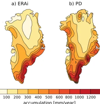
Fig. 3.Annual mean accumulation [mm yr−1_{] over the Greenland}

Ice Sheet for(a)ERAi and(b)PD simulation.

beforehand. Note also that a fixed present-day calendar was used to define the seasonal mean values of all simulations.

3 Greenland accumulation in different climate states

3.1 Present-day accumulation

(6)

Table 2.Annual means of hydrological parameters in [mm yr−1] averaged over the Greenland Ice Sheet.

Simulation Total Snowfall Sublimation Accumulation precipitation

PD 471 400 54 346

PI 390 344 40 303

EHPD 419 351 50 301

EH7ka 419 350 57 293

EH8ka 383 316 56 260

EH9ka 373 327 47 280

LGM 113 105 17 88

clearly overestimates (∼15 %) accumulation on average. Nevertheless, the spatial distribution of accumulation (both mean and variability) in the PD model simulation mainly re-sembles the observed distribution. Thus, we are sufficiently confident in using the CCSM4 model for studying GrIS ac-cumulation during past climate states.

3.2 Accumulation during the early Holocene and the LGM

To gain a first impression of Greenland accumulation during past climate conditions, we compare the EHPDand the LGM simulations against PI, i.e., the reference for the paleosimu-lations. The climate in EHPDis comparable to the one in the PMIP2 mid-Holocene simulations (Braconnot et al., 2007) as the orbital forcing is the dominant factor. The NH EHPD climate has an enhanced seasonal cycle, i.e., warmer sum-mers and colder winters particularly over continental areas compared to PI. In the Arctic Ocean, however, the summer warming leads to a warming of the northern high latitudes all year round due to feedback mechanisms, e.g., albedo-induced warming due to decreased NH sea ice in all seasons, similar to the findings by Fischer and Jungclaus (2011). The changes in the hydrological cycle in Greenland are more di-verse: during winter, snowfall increases along the Greenland east coast due to the increased moisture availability and mod-erate atmospheric circulation changes, which lead to stronger flow to Greenland from the east (not shown). In summer, the EHPDexhibits a distinct increase in precipitation in most of Greenland coming along with the summer warming. How-ever, precipitation that occurs along coastal regions and par-ticularly in southern Greenland falls mostly in the form of rain due to the warmer temperatures. Hence most of the pre-cipitation increase is not relevant for snow accumulation. The resulting annual mean snowfall (Fig. 4a) increases over in-land Greenin-land along the main ridge and at the east coast. Along the rest of the coastal areas we find rather a decrease in snowfall at the expense of rain. The increased tempera-tures also lead to stronger sublimation in these lower areas along the coast (not shown) contributing to the accumulation pattern in Fig. 4c, with lower accumulation in coastal areas except for the southeast. There, as well as for most of central

Fig. 4. Annual mean (a, b) snowfall and (c, d) accumulation [mm yr−1] anomalies for EHPD-PI and LGM-PI. Stippling denotes

values significant at the 5 % level based ont_{-test statistics.}

Greenland, the increased snowfall leads to higher accumula-tion in EHPD than for PI. The GrIS mean values (Table 2) show that the spatially diverse accumulation changes almost compensate each other, and as a result the GrIS mean accu-mulation rate for EHPDremains at the PI level.

(7)

Fig. 5.Early Holocene ice sheet sensitivity of annual mean(a, b, c)snowfall and(d, e, f)accumulation [mm yr−1] for the simulations with 7, 8, and 9 ka ice sheet topography. All values are anomalies from the basic early Holocene simulation (EHPD) with the present-day Greenland

Ice Sheet. Stippling denotes values significant at the 5 % level based ont_{-test statistics.}

extensive Laurentide Ice Sheet, the Atlantic storm track is shifted southwards (Hofer et al., 2012a, b). Therefore, North Atlantic areas that presently experience a lot of precipita-tion (southern Greenland, British Isles, Scandinavia) have a much drier climate during the LGM. The GrIS mean values of the hydrological cycle (Table 2) show a drop to approxi-mately 30 % of the PI levels in all quantities, proving that the interglacial–glacial difference in Greenland accumulation is remarkable.

3.3 Sensitivity to moderate changes in GrIS topography

To quantify the effect of the different Holocene ice sheet masks on GrIS accumulation, we compare the EH simu-lations with paleotopographies (EH7ka, EH8ka and EH9ka) against EHPDto identify the pure ice sheet sensitivity with all other boundaries conditions held constant. In all experi-ments, we observe a remarkable influence of the ice sheet to-pography on GrIS snowfall (Fig. 5a–c). Dominated by these changes in snowfall, accumulation changes equivalently in all three EH simulations with paleotopographies (Fig. 5d–f).

(8)

Fig. 6.Early Holocene ice sheet sensitivity of annual mean(a, b, c)2 m temperature [◦C] and(d, e, f)wind divergence [10−6s−1] over the Greenland Ice Sheet for the simulations with 7, 8 and 9 ka ice sheet topography. All values are anomalies from the basic early Holocene simulation (EHPD) with present-day Greenland Ice Sheet. Stippling in(a, b, c)denotes values significant at the 5 % level based ont-test

statistics. In(d, e, f)the shading denotes wind divergence at 850 hPa and contour lines represent wind divergence at 500 hPa with negative contours stippled and no zero line shown. Areas with negative (positive) wind divergence at the surface (at higher levels) experience local upward flow. Vice versa, areas with positive (negative) wind divergence at the surface (at higher levels) experience local downward flow.

Thereby both EH7ka and EH8ka exhibit changes in the an-nual mean circulation, which result in an enhanced east-erly flow towards Greenland (not shown). Similar to EHPD -PI (Fig. 4a), this leads to increased snowfall. (Fig. 4a), this anomalous westward flow leads to increased snowfall over the steep slopes of eastern Greenland (particularly in EH7ka, Fig. 5a), whereas on the lee side (western Greenland) snow-fall is decreased. Regarding the GrIS mean accumulation rates (Table 2), the 8 ka ice sheet setup leads to a reduction of GrIS mean snowfall and accumulation, whereas EH7ka roughly remains on the EHPDlevel.

In the EH9ka simulation, the GrIS is about 500 m higher (Fig. 1c), particularly in coastal regions, making the flanks of the ice sheet even steeper. Over the main ice sheet body

(9)

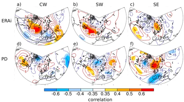
Fig. 7.z500 correlation and plus–minus composite patterns associated with annual mean accumulation in CW, SW, and SE for(a, b, c)ERAi and(d, e, f)the PD simulation. The shading illustrates the correlation pattern significant at the 5 % level (t_{-test statistics). Contour lines}

illustrate the z500 plus–minus composite pattern (in geopotential height meters). The plus–minus composite corresponds to the difference pattern of the±1 standard deviation samples of annual mean accumulation. The framed area in CW(a)indicates the North Atlantic domain used by the pattern correlation analysis.

4 Accumulation variability and its relationship to atmospheric circulation

4.1 Annual mean relationship

Besides changes due to various climate forcings in the mean accumulation, local accumulation shows remarkable interan-nual variability. As described in Sect. 2.5, we generate accu-mulation time series for four Greenland regions (Fig. 2) and calculate the correlation and plus–minus composite patterns to find links between local accumulation and atmospheric cir-culation variability. Hutterli et al. (2005) applied this method to ERA40 annual mean data and found distinct large-scale atmospheric circulation patterns for three of four of these ac-cumulation records. For ERAi we find very similar patterns for these three regions (Fig. 7a): accumulation variability in the CW region is related to an inverted NAO pattern: positive accumulation anomalies are associated with a high-pressure blocking south of Greenland equivalent to a negative NAO-like pattern and vice versa for negative accumulation anoma-lies. The blocking of southern Greenland leads to an en-hanced flow to central-western Greenland and thus results in stronger local snowfall and eventually in increased lation. The circulation pattern associated with SW accumu-lation shows anomalously strong westerly flow to southern Greenland due to a low-pressure system over north Green-land and a high-pressure situation over the North Atlantic westwards of the British Isles. For high SE accumulation another blocking-like pattern is found with a high-pressure

system centered over the Norwegian Sea. The SE pattern further shows two low-pressure anomalies over the Labrador Sea and western Russia. The resulting circulation transports moist air masses to southeastern Greenland. Note that all three (CW, SW, and SE) patterns have also an imprint on the European climate due to their large-scale nature (see Hutterli et al., 2005 for more details). For accumulation in the NE re-gion we find a weak pattern (not shown) resembling the one found in Hutterli et al. (2005). These authors relate NE ac-cumulation variability rather to the local cyclone frequency than to a distinct large-scale circulation pattern.

(10)

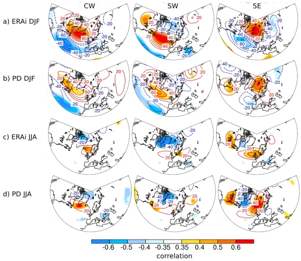
Fig. 8.z500 correlation and plus–minus composite patterns associated with seasonal mean accumulation in CW, SW, and SE for(a)ERAi winters (DJF),(b) PD winters,(c)ERAi summers (JJA), and(d) PD summers. As in Fig. 7, shading illustrates the correlation pattern significant at the 5 % level (t_{-test statistics) and contour lines illustrate the z500 plus–minus composite (in geopotential height meters). The}

plus–minus composite corresponds to the difference pattern of the±1 standard deviation samples of seasonal mean accumulation.

The CW accumulation of the model seems rather to be linked to a low-pressure system over north Greenland. The visual differences between the CW patterns of ERAi and PD are ev-ident by a very low pattern correlation (r_ERAi-PD₌−0.18). In contrast, for SW accumulation the model resembles the main pressure anomalies found in ERAi, which is reflected in a high pattern correlation ofr_ERAi-PD_{= 0.76. Hence, the model} indeed captures the relationship between local SW accumu-lation and the large-scale circuaccumu-lation found in the reanalysis. Regarding the SE pattern, the PD simulation represents to some extent the blocking over the Norwegian Sea and the low-pressure anomalies over the Labrador Sea and Russia found in ERAi. However the pattern correlation shows little agreement (r_ERAi-PD_{= 0.33) owing to the fact that the model} simulates a distinct low-pressure anomaly over central Eu-rope for high SE accumulation, a signal that cannot be found in reanalysis data.

Due to the limited ability of the model in simulat-ing the connection of local accumulation and atmospheric

circulation, the preconditions for testing the stability of these patterns in the paleosimulations within the model framework are not sufficiently reached (except for SW). To identify the origin of this model bias we extend the analysis to the sea-sonal and even daily timescale in order to check whether the model exhibits an improved capability of reproducing the link between Greenland accumulation and atmospheric cir-culation on shorter timescales.

4.2 Seasonal mean relationship

(11)

which is located south of Greenland in summer but over the Labrador Sea in the annual mean. However, the rest of the winter patterns and their annual equivalents show a high sim-ilarity, suggesting that winter variability is strongly recorded in the annual mean signal. All three winter patterns show a large-scale structure spanning the North Atlantic and at least partly the Europe domain. The summer (JJA) circula-tion patterns (Fig. 8c and d) exhibit much weaker pressure patterns, which is expected since the pressure variability in the warmer summer season is generally reduced compared to the winter season. Moreover, the summer patterns show few large-scale characteristics and are rather centered over Greenland. The summer CW pattern shows a weak cyclonic anomaly over north Greenland and a weak antipole south of Greenland, resulting in westerly flow to central Green-land. The SW pattern is somewhat similar but shifted to the south so that the snow falls over southwestern instead of central-western Greenland. Summer accumulation in the SE is associated with a wave-like pattern with high-pressure anomalies over the Great Lakes and east of Greenland and a low-pressure anomaly in between centered over the Labrador Sea. In contrast to the annual mean patterns (Fig. 7), the PD model simulation reproduces the ERAi patterns fairly well on the seasonal mean scale in both the winter (com-pare Fig. 8a and b) and the summer (com(com-pare Fig. 8c and d) season. The pattern correlation between the ERAi and PD winter plus–minus composites confirms this agreement, ex-hibiting the strongest conformance for CW (r_ERAi-PD_{= 0.88),} followed by SW (r_ERAi-PD_{= 0.64) and SE (}r_ERAi-PD_{= 0.52).} For the summer plus–minus composites the pattern corre-lation shows fairly high values for all three regions (CW: r_ERAi-PD_{= 0.60; SW:}r_ERAi-PD_{= 0.64; SE:}r_ERAi-PD_{= 0.52).}

The seasonal mean analysis is also conducted for spring (MAM) and autumn (SON). The resulting patterns (not shown) associated with regional accumulation variability are somewhat a transition between the summer and winter pat-terns. This is observed for both ERAi and PD. Further, when applying the correlation and plus–minus composites to sea-sonal mean precipitation instead of accumulation data, the resulting patterns (not shown) are equivalent to the seasonal patterns (Fig. 8) diagnosed from accumulation.

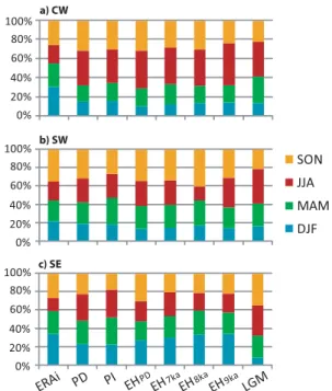
In the next step we address the question why the model’s ability in reproducing the ERAi annual patterns is limited (see Sect. 4.1), but at the same time the model’s seasonal circulation patterns coincide well with ERAi. The reason for this model–reanalysis disagreement is investigated by the analysis of the seasonal contributions to the annual signal. For all three regions, we find in ERAi and PD a substantial contribution of every season to the annual mean accumula-tion: for example, for CW accumulation in ERAi, each of the four seasons delivers at least 20 % of the total yearly ac-cumulation (not shown). Therefore the annual mean signal is interpreted as a mixture of all seasons and is (at least in present climate) not solely dominated by one season.

c) SE

0% 20% 40% 60% 80% 100%

0% 20% 40% 60% 80% 100% b) SW

a) CW

SON JJA MAM DJF

0% 20% 40% 60% 80% 100%

Fig. 9.Seasonal contribution to annual accumulation variability of the accumulation records in the(a)CW,(b)SW, and(c)SE region for ERAi and all simulations. Note that these seasonal contributions are calculated as standard deviations of the according seasonal mean accumulation time series. They are all expressed as relative portions of 100 %.

(12)

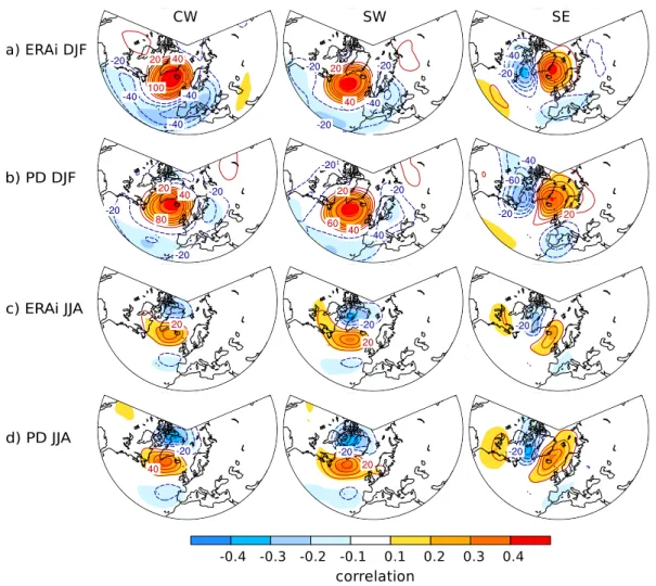
Fig. 10.z500 correlation and positive composite patterns associated with daily precipitation in CW, SW and SE for(a)ERAi winters (DJF),

(b)PD winters,(c)ERAi summers (JJA) and(d)PD summers. The shading illustrates the correlation pattern for values≥0.1 and≤ −0.1 (significant at the 1 % level due to the large sample size of≥2700 days for each season). Contour lines illustrate the z500 positive composite (in geopotential height meters) expressed as anomaly from seasonal mean z500. The positive composite samples all days with≥1 standard deviation in daily precipitation.

CW and SE annual plus–minus composites (Fig. 7) is mainly a problem of weighting the seasonal contributions rather than the representation of the large-scale circulation pattern con-nected with local GrIS accumulation.

4.3 Recorded circulation patterns in precipitation events

To ascertain the influence of atmospheric circulation on lo-cal Greenland accumulation, we extend our investigations to the daily (weather) timescale. For this purpose we identify the z500 circulation patterns associated with a local precip-itation event, defined as a day on which precipprecip-itation is≥1 standard deviation. Thereby the resulting circulation patterns in ERAi are the same regardless of whether the analysis is ap-plied to total precipitation or solely snowfall events (for the model this comparison is not possible due to a lack of daily snowfall output). For both ERAi and the PD simulation we

(13)

Table 3.Pattern correlation values of z500 composites for each model simulation vs. the present-day (PD) simulation. The composite patterns are derived from the accumulation (annual and seasonal mean) and precipitation (daily) time series for the CW, SW, and SE regions. The PD composite patterns used as reference to compare with are the ones shown in Fig. 10b and d (for daily precipitation variability in winter (DJF) and summer (JJA)), Fig. 8b and d (for winter and summer mean accumulation variability), and Fig. 7d–f (for annual mean accumulation variability). The domain used for the pattern correlation covers the North Atlantic area and Europe (see frame in Fig. 7). Note that bold values are significant at the 5 % level using a conservative estimate derived fromt_{-test statistics and autocorrelation applied on the North}

Atlantic domain composites.

Simulation DJF daily precipitation JJA daily precipitation DJF mean accumulation JJA mean accumulation Annual mean accumulation

CW SW SE CW SW SE CW SW SE CW SW SE CW SW SE

PI 0.96 0.96 0.96 0.92 0.97 0.95 0.86 0.52 0.57 0.55 0.76 0.85 0.24 0.40 0.77

EHPD 0.97 0.98 0.97 0.95 0.95 0.95 0.87 0.75 0.59 0.76 0.68 0.78 0.15 0.45 0.59

EH7ka 0.96 0.92 0.96 0.95 0.95 0.97 0.84 0.71 0.77 0.52 0.58 0.87 0.03 0.65 0.49

EH8ka 0.90 0.90 0.94 0.95 0.97 0.95 0.18 0.27 0.47 0.65 −0.10 0.61 0.29 0.57 0.77

EH9ka 0.97 0.97 0.95 0.96 0.97 0.96 0.66 0.79 0.78 0.65 0.61 0.50 0.04 0.31 0.84

LGM 0.72 0.94 0.80 0.78 0.82 0.65 0.71 0.78 0.20 0.53 0.58 0.26 0.09 0.40 0.69

linked to the so-called Scandinavian blocking pattern (Yiou et al., 2012) with a cyclonic system southwest of Greenland and a blocking over the Norwegian Sea. The resulting circu-lation transports relatively warm and moist air to SE Green-land. For the summer season (Fig. 10c and d), we find again weaker pressure patterns that resemble the patterns found in the seasonal mean analysis. All summer patterns are spatially limited to Greenland’s vicinity and hardly include any signal in the North Atlantic domain. CW and SW precipitation re-sults from westerly wind conditions caused by a low-pressure anomaly on the north side and a high-pressure anomaly on the south side of the precipitation region. Precipitation in the SE region is associated with the same wave-like pat-tern found for summer mean accumulation (Fig. 8c and d). Thereby moist air is advected from the south to the steep slopes in SE Greenland, where precipitation occurs.

All daily circulation patterns of the PD simulation (Fig. 10b and d) highly agree with the ERAi equivalents (Fig. 10a and c). The pattern correlation of the z500 positive composites for the North Atlantic domain shows very high values for all six patterns (0.81≤r_ERAi-PD≤0.98). The re-markable degree of consistency is explained by the fact that the daily patterns are based on an extensive sample (over 2700 daily values) compared to just 30 seasonal or annual mean values used in Sects. 4.1 and 4.2.

4.4 Stability during past climate states

Local GrIS precipitation and accumulation variability on var-ious timescales is significantly linked to specific circulation patterns as illustrated in the previous sections. Further, the climate model is to some extent capable of reproducing the patterns found in the ERAi reanalysis. However, to take up the idea of reconstructing atmospheric circulation variabil-ity from Greenland accumulation data or precipitation prox-ies, we further assess the stability of these relationships. In doing so, the PD composites for the annual, seasonal and daily accumulation/precipitation indices are compared with

the patterns of the paleoclimate simulations (Table 3). The stability is again quantified by the pattern correlation for the North Atlantic domain as in Sects. 4.1–4.3.

The highest agreement among the patterns from the differ-ent simulations is found for daily precipitation (see Fig. 10c and d for PD patterns). During both the winter and summer season, the precipitation events in the PI and all EH sim-ulations show the same positive composite patterns as PD, which is confirmed by pattern correlation values≥0.90 (see Table 3). Daily LGM patterns are also in agreement with PD (0.65≤r_PD-LGM≤0.94). This means that although the NH atmospheric circulation during the LGM strongly dif-fers from the present-day conditions (Hofer et al., 2012b), the relative daily weather patterns (anomalies from the sea-sonal means) that lead to precipitation over any of the three Greenland regions largely remain the same.

(14)

The summer plus–minus composite patterns demonstrate a reasonable consistency in all model simulations, with an average pattern correlation≥0.60. Exceptions are the EH8ka SW and LGM SE patterns. In the EH8kasimulation the orog-raphy of the 8 ka mask leads to an almost complete lack of snowfall and accumulation (partly at the expense of rain) in SW Greenland during the summer season. This signal is also reflected in the annual mean EH8ka–EHPDanomaly (Fig. 5b and e). Thus, the SW accumulation variability signal and the related z500 composites are not very trustworthy. Comparing the SW plus–minus composites based on precipitation of PD and EH8ka(not shown), the pattern correlation is 0.89, show-ing that there is no fundamental change in the connection of SW precipitation and the circulation pattern for EH8ka sum-mers, as also indicated by the stability of the daily patterns.

For the annual mean accumulation patterns we find limited stability throughout the model simulations (see Table 3, up-per left part). In particular, the annual mean CW z500 plus– minus composite shows almost no consistency with pattern correlation values below 0.3 for all comparisons. However, as discussed in Sects. 4.1 and 4.2 the CW patterns in the PD simulation clearly differ from the ERAi pattern due to the overestimation of the summer accumulation variability (see Fig. 9). Accordingly, the model’s CW annual patterns should be treated with caution. Regarding the SW annual patterns we observe medium stability throughout the model simula-tions. Thereby we identify good agreement around Green-land but less agreement over Europe and other more distant regions. The highest pattern correlations are found for the SE region, making accumulation in this area the only an-nual mean signal found to be consistently linked with the same large-scale atmospheric pattern in all simulated climate states. For the CW and SW regions, however, a stable rela-tionship between the annual accumulation variability signal and the associated circulation pattern is not confirmed by the model results.

As already presented in Sect. 4.2, seasonality within the relationship of local GrIS accumulation and the atmospheric circulation is a major issue. Since the annual mean accumula-tion signal adds together substantial poraccumula-tions of all four sea-sonal variability signals, a change in the contribution of each season to the annual signal is a critical quantity. As a con-sequence, even if the accumulation–atmospheric-circulation links remain stable throughout the different climate states during each season, differences in the relationship of the sea-sonal to the annual signal can cause the latter to be unsta-ble as discussed in Sect. 4.2. Assessing the seasonality in the model simulations shows that the seasonal contributions to the annual variability signal vary among the different cli-mate states (Fig. 9). Thereby the seasonal contributions ex-hibit sensitivity to the various forcings, so either changes in the orbital parameters or changes in the Greenland orogra-phy can have an impact on the interseasonal distribution of accumulation variability. In most cases the seasonal variabil-ity contribution to the annual accumulation signal goes along

with the change in the mean accumulation; for example, with a relative increase of summer accumulation at the expense of winter mean accumulation we observe an equivalent shift in the variability signal. During the early Holocene the orbital forcing leads to an increase in the CW summer accumula-tion, whereas the accumulation in the other seasons is rather decreased. This results in a larger contribution of summer variability in the annual accumulation signal (Fig. 9a). The SE winter accumulation during the LGM almost completely vanishes due to the glacial shift in the storm track, so the win-ter accumulation variability signal contribution to the annual signal is highly decreased (see Fig. 9c).

5 Discussion

As seen in Sect. 3, GrIS accumulation is strongly influenced by various forcing factors. Thereby, the differences in mean accumulation between PI and EHPD(see Fig. 4c) and among all EH simulations (see Fig. 5d–f) exhibit strong spatial vari-ability, emphasizing that accumulation records from differ-ent ice core sites can differ even on cdiffer-entennial to millen-nial timescales. This is especially true during time periods of changing GrIS topography (such as the early Holocene) when any change in ice sheet topography, in particular if al-tering the position of the marginal slopes, has a strong im-pact on local (mainly orographically induced) precipitation (see Fig. 5). In contrast, accumulation reacts rather uniformly to LGM conditions, where we observe a strong decrease all over Greenland compared to preindustrial conditions (see Fig. 4d). This means that accumulation records from dif-ferent Greenland sites are expected to synchronously regis-ter the glacial–inregis-terglacial cycles but can still vary on long timescales (centennial or millennial). Moreover, the indepen-dence between different regions is particularly strong regard-ing short-term (daily to interannual) accumulation variabil-ity as previously shown by Hutterli et al. (2005), whose re-gional accumulation indices are not significantly correlated with each other (with the exception of CW and SW).

To discuss the variety of climate signals included in such an accumulation record, we calculate the accumulation time series for three of the four Greenland regions (Fig. 11) using the model simulations. Note that due to the time-slice setup, the records are not continuous. Still they show the impact of different forcing factors on the local accumulation signal. Due to the spatial independence the three records only coin-cide with respect to some forcings (e.g., recent GHG increase or glacial conditions of LGM) but show little agreement re-garding the ice sheet sensitivity and interannual variability.

(15)

Fig. 11. Annual mean accumulation [mm yr−1] records for the

(a)CW,(b)SW, and (c)SE Greenland region based on the dif-ferent model simulations. The solid reference lines denote the 30 yr time-slice mean accumulation, whereas the stippled lines denote±1 standard deviation values. Note that due to the time-slice setup, the records are not continuous. In(a), the blue dots with error bars in-dicate the NGRIP accumulation rates determined for present day, the preindustrial era, and 7, 8, 9, and 21 ka. The present NGRIP accumulation rate of 190 m yr−1has been determined by NGRIP members (2004).

ice thicknessH_{= 3085 m ice equivalent (NGRIP members,} 2004) and the model parameterh_{= 500 m ice equivalent. A} density of 0.85 kg L−1_{is used for the depth where} preindus-trial ice is found and 0.917 kg L−1_{for the early Holocene and} the LGM in order to convert to accumulation rates in m water equivalent.

With respect to PD, the mean accumulation in all three regions in the PI simulation is reduced by about 20–30 %, which is explained by a cooler and drier climate all over the NH polar regions simulated for PI conditions. The PI–PD mean accumulation difference has to be regarded as thermo-dynamically driven as we see no major change in the mean circulation. We expect that the mean accumulation difference is larger in the simulations representing equilibrium states than in observations due to the fact that part of the response to the PI–PD GHG forcing in the real world is still not fully

active. However, the NGRIP as well as the NASA-U accu-mulation record (Anklin et al., 1998), which originate in the CW area (see Fig. 2), exhibit an increase in accumulation from preindustrial time to the present period. This is in agree-ment with the simulated CW accumulation response to global warming.

Comparing the PI with the EHPDaccumulation records, the early Holocene orbital forcing is observed to lead to a small increase in all three region’s mean accumulation. Here, the accumulation growth is induced by the insolation-forced warmer summer temperatures during the early Holocene leading to an enhanced hydrological cycle and an increase in snowfall (see Fig. 4a) and consequently more accumu-lation, particularly in the CW and SE region. The different ice sheet topographies in the EH sensitivity simulations also exhibit a distinct influence on the mean accumulation in all three records. This reveals that the amount of accumulation is very sensitive to changes in the local orography and that already comparatively small changes in GrIS topography are clearly reflected in the accumulation signal. Since changes in topography have a very local signature, they are one rea-son why accumulation records from different Greenland re-gions are not expected to conform on centennial to millennial timescales. For example, CW accumulation occurring with 7 ka topography is about 15 % higher than the equivalent with present topography (compare EH7ka and EHPDin Fig. 11a), whereas in the SW region (Fig. 11b) accumulation in EH7ka is reduced by about 50% with respect to EHPD. CW accumu-lation simulated in EH7ka, EH8ka, and EH9ka agrees reason-ably with NGRIP data for 7, 8, and 9 ka, respectively. The model results suggest that the observed increase in NGRIP accumulation from 9 to 7 ka might be caused by changes in the local topography.

As expected, the largest difference in accumulation is recorded for changes between the interglacial and glacial climate states. In all three regions we observe an average drop from PI to LGM of about 80 %, which is in agreement with the NGRIP data. As already identified by Kapsner et al. (1995), the glacial–interglacial differences cannot solely be explained by thermodynamic effects. In the case of the LGM simulation, the presence of an extensive Laurentide ice sheet reveals a distinct reorganization of the atmospheric circula-tion. In agreement with Pausata et al. (2011), we observe weaker westerly winds over the high-latitudinal North At-lantic and a southward shift in the storm tracks (Hofer et al., 2012a), which leads to an amplification of the drying con-ditions over Greenland. Langen and Vinther (2009) further show that the moisture sources at Greenland ice core sites differ substantially for LGM compared to present-day condi-tions, also supporting the important role of dynamics in ex-plaining the glacial–interglacial precipitation differences.

(16)

can be attributed to dynamical features, i.e., variability in the atmospheric circulation. Following the idea of Hutterli et al. (2005), we test whether years with anomalously high accumulation (spikes above upper dashed lines in Fig. 11) are consistently accompanied by the same atmospheric pat-tern with respect to years with anomalous low accumulation (spikes below lower dashed lines in Fig. 11). However, the circulation patterns accounting for the annual accumulation variability are not stable in all simulated climate states due to subseasonal effects. One caveat, however, is the fact that the model shows limited ability in reproducing the circula-tion patterns found for the reanalysis (Fig. 7), in particular for the accumulation variability in the CW region. The ex-pansion of the analysis to the seasonal scale reveals that the model is actually able to reproduce the atmospheric patterns responsible for accumulation variability within the different seasons. Furthermore, the model agrees with ERAi regarding the daily circulation–accumulation relationship on the syn-optic scale. This increases our confidence that the model cap-tures the dynamical situation leading to a precipitation event. The model’s difficulties in the representation of the annual relationship are attributed to differences in the contribution of the different seasons to the annual variability signal (see Sect. 4.2 for more details).

Despite these model limitations, we have confidence in the conclusion that the approach by Hutterli et al. (2005) is not necessarily valid for different climate states: the relationship between local GrIS accumulation and large-scale circulation patterns exhibits a remarkable seasonal cycle in both ERAi and the model simulations. Within a season, the attributed circulation patterns show good agreement in all paleosimu-lations. However, since the seasonal signals can add up dif-ferently to the annual signal (Fig. 9), we do not find a stable relationship between annual accumulation and annual circu-lation patterns except for the SE region. The contributions of the seasonal to the annual variability signal generally fol-lows the accumulation mean: if a change in seasonality due to an alteration in the orbital parameters, e.g., during the early Holocene, results in more GrIS summer accumulation at the expense of winter accumulation, the seasonal accu-mulation variability signals change accordingly. Hence, the seasonal contributions to the annual accumulation variability in any Greenland region cannot be expected to be constant over longer time periods. This implies that the composites in the annual accumulation records (as indicated in the differ-ent time slices in Fig. 11) have to be treated very carefully regarding their interpretation since they likely differ due to subseasonal effects. The observed seasonality further indi-cates that using a proxy to describe the annual mean state of the atmospheric circulation is not very meaningful. It also links to the findings by Pausata et al. (2009), who showed that the annual cycle of precipitation at Greenland ice core sites is very different for the LGM compared to present-day conditions, which can cause a bias in annual mean tempera-ture estimates based on water isotopes.

6 Conclusions

In the course of this study, the sensitivity of GrIS accumu-lation to various forcings – e.g., changes in orbital forc-ing or the ice sheet topography – is presented by climate simulations for the present, the preindustrial era, the early Holocene, and the LGM. A second focus is set on the rela-tionship of local accumulation variability and large-scale cir-culation patterns and its stability throughout the paleosimu-lations. The obtained results have important implications for accumulation and other precipitation proxy records derived from Greenland ice cores: Greenland accumulation generally reacts very sensitively to all tested external forcing factors. Thereby, the accumulation changes due to different forcings exhibit strong spatial variability, showing that accumulation records from different ice core sites cannot be expected to be coherent since they include an important local charac-teristic. The only uniform accumulation signal throughout Greenland is the strong decrease for the glacial LGM condi-tions and the increase associated with the recent rise in GHG concentrations.

Changes in both the mean and year-to-year variability of accumulation are dominated by snowfall, whereas the impact of sublimation is an order of magnitude smaller. Changes in mean accumulation between different climate periods are driven by both thermodynamic and dynamic factors. Regard-ing the thermodynamic impact, a warmRegard-ing is generally ac-companied by an increase in precipitation. As long as this precipitation falls in the form of snow, the warming results in an accumulation increase as the increase in sublimation due to the warming cannot compensate for the additional snow mass. Dynamic drivers of accumulation changes are either changes in the large-scale circulation or in the local orogra-phy having a distinct imprint on the amount of precipitation deposited in any GrIS region. The variety of processes affect-ing precipitation and accumulation on Greenland is certainly a challenge for the interpretation of long-term records.

(17)

It is also shown that on the daily scale, a precipitation event in any of the tested Greenland regions is associated with the same weather situation in all climate states. Hence, we indeed see the potential to reconstruct seasonal circula-tion patterns from ice core data. This approach, however, requires a precipitation proxy that resolves single seasons and that is explicitly dominated by wet deposition. To our knowledge, such a proxy record has not been established yet. However, new high-resolution records of various chemical species from the NEEM ice core might offer the opportu-nity to reconstruct the occurrence of distinct seasonal large-scale circulation patterns as proposed in this work. As ac-cumulation variability at NEEM is significantly correlated to accumulation in the CW region (see Fig. 2), the atmo-spheric circulation patterns accounting for interannual accu-mulation/precipitation variability at NEEM are expected to look like the CW patterns. This can be confirmed by apply-ing the analysis to the NEEM region.

Acknowledgements. We acknowledge the Swiss National Su-percomputing Centre (CSCS) for providing the suSu-percomputing facilities. The ERA-Interim and ERA-40 reanalysis data were obtained from the European Centre for Medium-Range Weather Forecasts (ECMWF) data archive. This work is supported by fund-ing to the Past4Future project from the European Commission’s 7th Framework Programme, grant number 243908 (2010–2014).

Edited by: V. Rath

References

Andersen, K. K., Svensson, A., Johnsen, S. J., Rasmussen, S. O., Bigler, M., Rothlisberger, R., Ruth, U., Siggaard-Andersen, M. L., Steffensen, J. P., Dahl-Jensen, D., Vinther, B. M., and Clausen, H. B.: The Greenland Ice Core Chronology 2005, 15– 42 ka, Part 1: constructing the time scale, Quaternary Sci. Rev., 25, 3246–3257, doi:10.1016/j.quascirev.2006.08.002, 2006. Anklin, M., Bales, R. C., Mosley-Thompson, E., and Steffen, K.:

Annual accumulation at two sites in northwest Greenland during recent centuries, Journal of Geophysical Research-atmospheres, 103, 28775–28783, doi:10.1029/98JD02718, 1998.

Appenzeller, C., Stocker, T. F., and Anklin, M.: North Atlantic os-cillation dynamics recorded in Greenland ice cores, Science, 282, 446–449, doi:10.1126/science.282.5388.446, 1998.

Bales, R. C., Guo, Q. H., Shen, D. Y., McConnell, J. R., Du, G. M., Burkhart, J. F., Spikes, V. B., Hanna, E., and Cappelen, J.: Annual accumulation for Greenland updated using ice core data developed during 2000–2006 and analysis of daily coastal meteorological data, J. Geophys. Res.-Atmos., 114, D06116, doi:10.1029/2008JD011208, 2009.

Banta, J. R. and McConnell, J. R.: Annual accumulation over recent centuries at four sites in central Greenland, J. Geophys. Res.-Atmos., 112, D10114, doi:10.1029/2006JD007887, 2007. Berger, A. L.: Long-term Variations of Daily Insolation and

Quaternary Climatic Changes, J. Atmos. Sci., 35, 2362–2367, doi:10.1175/1520-0469(1978)035<2362:LTVODI>2.0.CO;2, 1978.

Braconnot, P., Otto-Bliesner, B., Harrison, S., Joussaume, S., Pe-terchmitt, J.-Y., Abe-Ouchi, A., Crucifix, M., Driesschaert, E., Fichefet, Th., Hewitt, C. D., Kageyama, M., Kitoh, A., Laîné, A., Loutre, M.-F., Marti, O., Merkel, U., Ramstein, G., Valdes, P., Weber, S. L., Yu, Y., and Zhao, Y.: Results of PMIP2 coupled simulations of the Mid-Holocene and Last Glacial Maximum – Part 1: experiments and large-scale features, Clim. Past, 3, 261– 277, doi:10.5194/cp-3-261-2007, 2007.

Chen, L. L., Johannessen, O. M., Wang, H. J., and Ohmura, A.: Accumulation over the Greenland Ice Sheet as repre-sented in reanalysis data, Adv. Atmos. Sci., 28, 1030–1038, doi:10.1007/s00376-010-0150-9, 2011.

Cruger, T., Fischer, H., and von Storch, H.: What do accumulation records of single ice cores in Greenland represent?, J. Geophys. Res.-Atmos., 109, D21110, doi:10.1029/2004JD005014, 2004. Dee, D. P., Uppala, S. M., Simmons, A. J., Berrisford, P., Poli,

P., Kobayashi, S., Andrae, U., Balmaseda, M. A., Balsamo, G., Bauer, P., Bechtold, P., Beljaars, A. C. M., van de Berg, L., Bid-lot, J., Bormann, N., Delsol, C., Dragani, R., Fuentes, M., Geer, A. J., Haimberger, L., Healy, S. B., Hersbach, H., Hólm, E. V., Isaksen, L., Kållberg, P., Köhler, M., Matricardi, M., McNally, A. P., Monge-Sanz, B. M., Morcrette, J.-J., Park, B.-K., Peubey, C., de Rosnay, P., Tavolato, C., Thépaut, J.-N., and Vitart, F.: The ERA-Interim reanalysis: configuration and performance of the data assimilation system, Q. J. Roy. Meteorol. Soc., 137, 553– 597, doi:10.1002/qj.828, 2011.

Dethloff, K., Schwager, M., Christensen, J. H., Kilsholm, S., Rinke, A., Dorn, W., Jung-Rothenhausler, F., Fischer, H., Kipfstuhl, S., and Miller, H.: Recent Greenland accumulation estimated from regional climate model simulations and ice core analysis, J. Cli-mate, 15, 2821–2832, 2002.

Fischer, N. and Jungclaus, J. H.: Evolution of the seasonal tempera-ture cycle in a transient Holocene simulation: orbital forcing and sea-ice, Clim. Past, 7, 1139–1148, doi:10.5194/cp-7-1139-2011, 2011.

Gent, P. R., Danabasoglu, G., Donner, L. J., Holland, M. M., Hunke, E. C., Jayne, S. R., Lawrence, D. M., Neale, R. B., Rasch, P. J., Vertenstein, M., Worley, P. H., Yang, Z. L., and Zhang, M. H.: The Community Climate System Model Version 4, J. Climate, 24, 4973–4991, doi:10.1175/2011JCLI4083.1, 2011.

Hakuba, M. Z., Folini, D., Wild, M., and Schar, C.: Impact of Green-land’s topographic height on precipitation and snow accumu-lation in idealized simuaccumu-lations, J. Geophys. Res.-Atmos., 117, D09107, doi:10.1029/2011JD017052, 2012.

Hofer, D., Raible, C. C., Dehnert, A., and Kuhlemann, J.: The im-pact of different glacial boundary conditions on atmospheric dy-namics and precipitation in the North Atlantic region, Clim. Past, 8, 935–949, doi:10.5194/cp-8-935-2012, 2012a.

Hofer, D., Raible, C. C., Merz, N., Dehnert, A., and Kuhlemann, J.: Simulated winter circulation types in the North Atlantic and Eu-ropean region for preindustrial and glacial conditions, Geophys. Res. Lett., 39, L15805, doi:10.1029/2012GL052296, 2012b. Hunke, E. C. and Lipscomb, W. H.: CICE: The Los Alamos Sea

(18)

Hutterli, M. A., Raible, C. C., and Stocker, T. F.: Reconstruct-ing climate variability from Greenland ice sheet accumula-tion: An ERA40 study, Geophys. Res. Lett., 32, L23712, doi:10.1029/2005GL02474, 2005.

Hutterli, M. A., Crueger, T., Fischer, H., Andersen, K. K., Raible, C. C., Stocker, T. F., Siggaard-Andersen, M. L., McConnell, J. R., Bales, R. C., and Burkhart, J. F.: The influence of regional circulation patterns on wet and dry mineral dust and sea salt de-position over Greenland, Clim. Dynam., 28, 635–647, 2007. Kapsner, W. R., Alley, R. B., Shuman, C. A., Anandakrishnan, S.,

and Grootes, P. M.: Dominant Influence of Atmospheric Cir-culation On Snow Accumulation In Greenland Over the Past 18,000 Years, Nature, 373, 52–54, doi:10.1038/373052a0, 1995. Langen, P. L. and Vinther, B. M.: Response in atmospheric circula-tion and sources of Greenland precipitacircula-tion to glacial boundary conditions, Clim. Dynam., 32, 1035–1054, doi:10.1007/s00382-008-0438-y, 2009.

Lehner, F., Raible, C. C., and Stocker, T. F.: Testing the ro-bustness of a precipitation proxy-based North Atlantic Os-cillation reconstruction, Quaternary Sci. Rev., 45, 85–94, doi:10.1016/j.quascirev.2012.04.025, 2012.

Luterbacher, J., Xoplaki, E., Dietrich, D., Jones, P. D., Davies, T. D., Portis, D., Gonzalez-Rouco, J. F., von Storch, H., Gyalistras, D., Casty, C., and Wanner, H.: Extending North Atlantic Oscilla-tion reconstrucOscilla-tions back to 1500, Atmos. Sci. Lett., 2, 114–124, doi:10.1006/asle.2001.0044, 2001.

McConnell, J. R., Arthern, R. J., Mosley-Thompson, E., Davis, C. H., Bales, R. C., Thomas, R., Burkhart, J. F., and Kyne, J. D.: Changes in Greenland ice sheet elevation attributed pri-marily to snow accumulation variability, Nature, 406, 877–879, doi:10.1038/35022555, 2000a.

McConnell, J. R., Mosley-Thompson, E., Bromwich, D. H., Bales, R. C., and Kyne, J. D.: Interannual variations of snow accumula-tion on the Greenland Ice Sheet (1985–1996): new observaaccumula-tions versus model predictions, J. Geophys. Res.-Atmos., 105, 4039– 4046, doi:10.1029/1999JD901049, 2000b.

Merkel, U., Prange, M., and Schulz, M.: ENSO variability and tele-connections during glacial climates, Quaternary Sci. Rev., 29, 86–100, doi:10.1016/j.quascirev.2009.11.006, 2010.

Mosley-Thompson, E., McConnell, J. R., Bales, R. C., Lin, P. N., Steffen, K., Thompson, L. G., Edwards, R., and Bathke, D.: Lo-cal to regional-sLo-cale variability of annual net accumulation on the Greenland ice sheet from PARCA cores, J. Geophys. Res.-Atmos., 106, 33839–33851, doi:10.1029/2001JD900067, 2001. Neale, R. B., Richter, J., Park, S., Lauritzen, P. H., Vavrus, S. J.,

Rasch, P. J., and Zhang, M.: The Mean Climate of the Commu-nity Atmosphere Model (CAM4) in Forced SST and Fully Cou-pled Experiments, J. Climate, 26, 5150–5168, doi:10.1175/JCLI-D-12-00236.1, 2013.

NGRIP members: High-resolution record of Northern Hemisphere climate extending into the last interglacial period, Nature, 431, 147–151, doi:10.1038/nature02805, 2004.

Oleson, K., Lawrence, D., Bonan, G., Flanner, M., Kluzek, E., Lawrence, P., Levis, S., Swenson, S., Thornton, P., Dai, A., Decker, M., Dickinson, R., Feddema, J., Heald, C., Hoffman, J.-F., Mahowald, N., Niu, G.-Y., Qian, T., Randerson, J., Running, S., Sakaguchi, K., Slater, A., Stockli, R., Wang, A., Yang, Z.-L., Zeng, X., and Zeng, X.: Technical Description of version 4.0

of the Community Land Model (CLM), NCAR Technical Note NCAR/TN-478+STR, doi:10.5065/D6FB50WZ, 2010. Pausata, F. S. R., Li, C., Wettstein, J. J., Nisancioglu, K. H., and

Battisti, D. S.: Changes in atmospheric variability in a glacial climate and the impacts on proxy data: a model intercomparison, Clim. Past, 5, 489–502, doi:10.5194/cp-5-489-2009, 2009. Pausata, F. S. R., Li, C., Wettstein, J. J., Kageyama, M., and

Ni-sancioglu, K. H.: The key role of topography in altering North Atlantic atmospheric circulation during the last glacial period, Clim. Past, 7, 1089–1101, doi:10.5194/cp-7-1089-2011, 2011. Peltier, W. R.: Global glacial isostasy and the surface of the

ice-age earth: The ice-5G (VM2) model and grace, An-nual Review of Earth and Planetary Sciences, 32, 111–149, doi:10.1146/annurev.earth.32.082503.144359, 2004.

Pinto, J. G. and Raible, C. C.: Past and recent changes in the North Atlantic oscillation, Wiley Interdisciplinary Reviews, Climate Change, 3, 79–90, doi:10.1002/wcc.150, 2012.

Raible, C. C., Casty, C., Luterbacher, J., Pauling, A., Esper, J., Frank, D. C., Buntgen, U., Roesch, A. C., Tschuck, P., Wild, M., Vidale, P. L., Schar, C., and Wanner, H.: Climate variability-observations, reconstructions, and model simulations for the Atlantic-European and Alpine region from 1500–2100 AD, Cli-matic Change, 79, 9–29, doi:10.1007/s10584-006-9061-2, 2006. Rogers, J. C., Bathke, D. J., Mosley-Thompson, E., and Wang, S. H.: Atmospheric circulation and cyclone frequency variations linked to the primary modes of Greenland snow accumulation, Geophys. Res. Lett., 31, L23208, doi:10.1029/2004GL021048, 2004.

Smith, D., Harrison, S., Firth, C., and Jordan, J.: The early Holocene sea level rise, Quaternary Sci. Rev., 30, 1846–1860, 2011. Uppala, S. M., Kallberg, P. W., Simmons, A. J., Andrae, U.,

Bech-told, V. D., Fiorino, M., Gibson, J. K., Haseler, J., Hernandez, A., Kelly, G. A., Li, X., Onogi, K., Saarinen, S., Sokka, N., Al-lan, R. P., Andersson, E., Arpe, K., Balmaseda, M. A., Beljaars, A. C. M., Van De Berg, L., Bidlot, J., Bormann, N., Caires, S., Chevallier, F., Dethof, A., Dragosavac, M., Fisher, M., Fuentes, M., Hagemann, S., Holm, E., Hoskins, B. J., Isaksen, L., Janssen, P. A. E. M., Jenne, R., McNally, A. P., Mahfouf, J. F., Mor-crette, J. J., Rayner, N. A., Saunders, R. W., Simon, P., Sterl, A., Trenberth, K. E., Untch, A., Vasiljevic, D., Viterbo, P., and Woollen, J.: The ERA-40 re-analysis, Q. J. Roy. Meteorol. Soc., 131, 2961–3012, doi:10.1256/qj.04.176, 2005.

Varma, V., Prange, M., Merkel, U., Kleinen, T., Lohmann, G., Pfeif-fer, M., Renssen, H., Wagner, A., Wagner, S., and Schulz, M.: Holocene evolution of the Southern Hemisphere westerly winds in transient simulations with global climate models, Clim. Past, 8, 391–402, doi:10.5194/cp-8-391-2012, 2012.

Yeager, S. G., Shields, C. A., Large, W. G., and Hack, J. J.: The low-resolution CCSM3, J. Climate, 19, 2545–2566, doi:10.1175/JCLI3744.1, 2006.