Pressure evolution inside a cork stopper under vacuum Nenad Bundaleski, Ana L. Fonseca and Orlando M.N.D. Teodoro
CEFITEC, Departamento de Física, Faculdade de Ciências e Tecnologia, Universidade Nova de Lisboa, P-2829-516, Campus de Caparica, Caparica, Portugal
Abstract
A cork stopper maybe described by a 3D array of microcavities, which is a 3D arrangement of small cavities interconnected by tiny restrictions. Upon a step pressure change gas slowly flows through the restrictions from the microcavities to the exterior. In this work, we describe a technique to calculate the pressure evolution inside the array and the total gas flow. It is based on electrical analogies and uses a SPICE simulation software to solve large arrays. We reveal how to convert orthogonal 3D arrays in 1D arrays based on symmetry considerations, allowing us to simulate very large systems. We then apply our technique to a cork stopper to calculate the pressure evolution in the inner cell when the stopper is subjected to vacuum. We also describe an experiment to measure the characteristic time constant of a cork stopper and we compare the experimental results with those obtained from our simulations.
Keywords
Gas flow, flow simulation, pressure simulation, 3D array, cork 1. Introduction
Cellular materials may be described as an array of small cavities fully or partially closed. The transport of gases through this media is slightly different of that through porous materials, because of the individual cell volumes. These cavities are huge sources of gas changing the transient response of the gas flow. Physical systems consisting of volumes in the micrometer range interconnected by narrow channels are here denoted as 3D microcavity arrays. Good examples of these materials are foams, sponges and cork. Although the motivation for this work came from the need to understand the pressure evolution in cork cells when subject to vacuum, the proposed approach is valid for any kind of 3D arrays.
Cork is a well-known cellular material; while the cell walls are still present in the dead biological cells, their interior is hollowed of cytoplasm and filled with gas. Although cork is usually referred as impermeable and commonly used to seal, its permeability for many gases and vapors is well known [1-3]. Cells are not completely closed since very small channels (plasmodesma, plural: plasmodesmata) in the cell walls interconnect the volumes of plant cells [4]. It has been proposed that these channels play a major role in the transport of gases when cork is not compressed [1]. Therefore, cork may be roughly described as a 3D arrangement of cubic cells with 30 µm per side and walls 1.5 µm thick with small channels across as described in references [1] and [5]. These references also describe the permeation experiments, which were performed, showing that gas flow could be explained by many small conductances in parallel and in series. In a typical experiment, a sample of cork having a permeation area of 9.6 mm2 and a thickness of 2.15 mm was
exposed to 1 bar of He and the leak rate was measured by an a helium leak detector mass spectrometer. Such sample corresponds to 10690 cubic cells in parallel and 72 cells in series. The measured flow rate for this sample was 1×10!! mbar.L/s. If we assume that
cells are interconnected by a single restriction then the individual conductance can be calculated as 7×10!!! L/s. The same experiment was repeated for more than 100 samples,
showing that this result was close to the mean value.
Reference [5] also describes another permeation experiment in which different gases of molecular mass 𝑚 were tested by a pressure rise technique. The gas flow was proportional to 1/ 𝑚, which is typical of molecular flow. This is consistent with the diameter of the plasmodesmata of the order of 100 nm observed by electron microscopy [4]. These observations also showed that the channels are partially filled with a dense material, suggesting that the available free diameter is much smaller. Since the mean free path of air at atmospheric pressure is about 70 nm, collisions between air molecules in these small conduits are certainly rare. Therefore, it is reasonable to assume that conductance between cork cells is not pressure dependent under these conditions.
The average volume of cork cells is about 2×10-11 L. In a cork stopper there are about
7×10⁸ of these cells [6]. When the cork is subjected to vacuum, the gas inside the cells
will flow out through the surface cells. Gas from inside will flow to the outer cells and then to the exterior. Consequently, pressure in inner cells will slowly change. The inner is the cell the slower will be the rate of pressure change.
One of the key approximations introduced when working with 3D arrays of the order of the cork stopper is that all cells have equal volumes and all plasmodesmata have the same conductance. Although these conditions are not fulfilled for any natural material the calculations show that these approximations are reasonable when using mean cell volumes and mean plasmodesma conductances taken from permeation measurements. However, cork also has large inhomogeneities as lenticular channels and other natural defects. Due to their unknown variability, no efforts were done to consider them in the model and to perform uncertainty analysis. The mean values were taken from homogeneous pieces of cork without macroscopic defects. The influence of large defects on the gas flow can be however estimated by comparing calculation results with an experiment, as it will be shown in the experimental section.
The purpose of this work is, first, to achieve a useful qualitative description of the total flow as function of time coming out from a 3D array of interconnected cells, and secondly, to describe the pressure evolution at any point of the inner volume. The relevance of these goals is twofold: to describe the pressure evolution inside cork when exposed to vacuum in deodorization treatments and to describe its ability to store highly pressurized gas at room temperature. In the first case it is important to know the pressure in the most hidden cell to understand when the vapor pressure of critical odors is achieved; in the second case, to describe the total flow out of cork after a step pressure drop.
In addition, an experiment was performed in which a stopper was exposed to a step pressure change. Due to the gas release from the stopper, the pressure inside the container raised. The comparison of the experimental result with the calculation provides insight into relevant properties of cork and into the influence of defects on the gas flow from the cork stopper.
2. Model description
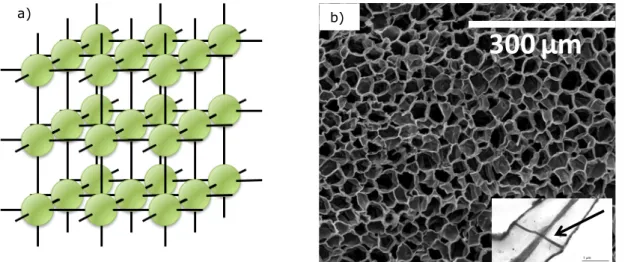
Let us assume that we have a 3D hollowed cellular material with equal volumes interconnected by equal small channels as depicted in Figure 1 a). Spheres are used to represent the volumes and the lines to represent the channels. Figure 1 b) shows an electron microscopy image of cork where the empty cells can be clearly seen as well as one channel across the cell wall (in the inset). Those volumes close to the borders are connected to the exterior by the same type of channels. Therefore, if we change the pressure outside, gas will flow and the pressure in every volume will change at a rate ruled by a time constant that is a function of its position in the 3D array. The pressure in those volumes closer to the border will change faster than those inside.
Figure 1- a) 3D array of 3×3×3 cells (spheres) connected by conductances (straight lines) between volumes and to the exterior. b) Electron microscopy image of cork; the inset shows one channel across the cell wall.
Upstream compartment
Downstream compartment
z
Figure 1A
Figure 1B
Gas flow
direction
x
y
z
x
y
Figure 1C
Figure 1D
Figure 1E
300 μm
300 μm
300 μm
b) a)2.1 Equivalent electrical circuit
It is well known that the pressure evolution in any vacuum system can be calculated by solving an equivalent electrical circuit, in which current I and voltages U correspond to gas flow Q and pressure p, respectively; the conductances are described by resistors (conductance= 1/R) and volumes by capacitors. When the gas flow is in the molecular regime, the equivalent resistors are constant. This approach was applied by several other authors to model gas distributions as well as for the simulation of rarefied gas dynamics [7,8]. Consequently, the problem of pumping a 3D array shown in Fig. 1 is equivalent to discharging (or charging) of a 3D array of 𝑛 capacitors with one end connected to ground and the other interconnected by resistors. All resistors at the border of the network are shunted and connected to ground via a switch. All capacitors are at the initial potential U0. The equivalence between the vacuum and electrical parameters is summarized in Table 1. The mathematical description of the time evolution of any voltage U in such configuration leads to a differential equation of nth order, which has an analytical solution of the type:
𝑈 𝑡 = 𝑎!𝑒! !! !" ! ! !!! Eq. 1
where 𝑛 is the total number of nodes (the same as the number of capacitors), 𝑡 the time, 𝑎! and 𝑏! are constants retrieved by solving the differential equation and RC the time
constant of a single RC circuit. Thus, the solution has as many terms as the number of nodes in the array.
The number of capacitors and resistors in a cubic 3D array with 𝑙 nodes along each side is given by
𝑚!"#= 𝑛!
𝑚!"#= 3𝑙!+ 3𝑙!
Eq. 2
Finding the analytical solution for large arrays becomes already very complicated for arrays having several nodes per side (cf. Eq. 1). For instance, an array having 20 nodes per side, has 8 000 capacitors and 25 200 resistors. Moreover, it is not practical the use of equations of that size (with 𝑛 terms) to calculate the total flow and the pressure evolution inside an arbitrary cell. For a cork stopper having about 109 cells, the solution given by Eq.
1 is the summation of 109 terms!
Table 1- Equivalence between gas flow and electrical quantities
Gas flow Electrical
Quantity Values for cork Quantity Values taken
Conductance, C 7×10-11 L/s ↔ Inverse of resistance, 1/R 1/(14.29 GΩ)
Volume, V 2×10-11 L ↔ Capacitance, C 20 pF
Initial pressure, p 1000 mbar ↔ Initial voltage, U0 1000 V
Initial flow rate, Q 7×10⁻⁸ mbar.L/s * ↔ Initial current, I 70 nA*
Time constant, V/Cd† 0.286 s ↔ R×C 0.286 s
• Maximum Q and I at t=0 (Q0=p×Cd; I0=U0/R) for a single conductance-volume or RC circuit.
• † Cd is the flow conductance of a single restriction.
The advantage of using electrical equivalents to describe gas flow and pressure evolution is because there are many options to simulate electrical circuits. The transient response of a RC network can be simulated by well-known SPICE codes (Simulation Program with Integrated Circuit Emphasis) [9]. SPICE is a well-proven electronic circuits simulation algorithm available via many commercial computer codes. In this work, freeware LTSPICE
IV, which is produced by the semiconductor manufacturer Linear Technology [10], was used to simulate 3D RC arrays as large as possible.
A search of similar problems in scientific databases returned empty for both, gas flow networks and RC networks. Therefore, we believe there are no publications addressing the same or a similar problem.
2.2 SPICE simulation of 3D RC networks
3D arrays are very difficult to represent and to visualize in a diagram. Therefore, for the sake of simplicity, a 2D array having 3×3 nodes is represented in Figure 2 to illustrate some relevant aspects of the simulation. At every node, there is one capacitor. Every node is connected to the neighbor node by a resistor. All resistors and all capacitors have the same value. Each resistor at the border is connected to the same point, the switch to ground. All capacitors were initially charged at U0. At time t=0, the switch was closed and the total current I(t) and the voltage at the inner node U(t) were recorded as a function of time.
The circuit is defined in a text netlist file fed to LTSPICE. This netlist describes each component and how it is connected in the circuit. The netlist has as many lines as the number of components plus one instruction to ask the simulator to perform the transient analysis. Since the netlist file quickly becomes very large and intricate, a code written in SCILAB programming language was written to generate this file.
This approach can be readily applied to an arbitrary geometry and provide exact calculation of the gas flow in the molecular regime. In addition, one can vary the capacitor and resistor values to follow some distribution without affecting the execution time. Its limitation is related to the number of nodes in the 3D array for which the calculations can be performed with a reasonable execution time. Indeed, increasing the number of nodes leads to circuits having enormous amounts of components, which becomes very heavy for ordinary desktop computers. To simulate a 3D array equivalent to a cork stopper, a few billions of components are required, what makes virtually impossible its simulation in any computer (the SPICE netlist would have billions of lines!). The number of nodes for which calculations can be performed in a reasonable execution time (few hours) on an ordinary PC is of the order of 104, corresponding to the volumes of the order of 1 mm3.
2.3 Pumping of a spherically symmetric 3D array – the shell model
In order to overcome the limitations of the approach described in the previous section, we consider a uniform 3D array (all capacitors and resistors having the same value) of a spherical shape. As it will be shown below, the spherical symmetry enables us to reduce the calculation to the 1D problem and consequently calculate the pumping of the volume equal to that of a stopper in a quite fast way by applying here the introduced shell model.
a) b)
Figure 2- a) A 2D RC array used to illustrate how the simulation was performed. All resistors at the border were connected in parallel to a switch. Colored nodes are symmetrically connected to the inner node. b) A 3D array may be described by concentric shells of equal volumes
Capacitors charged with U0 at t=0 I(t) = ?
interconnected by small conductances
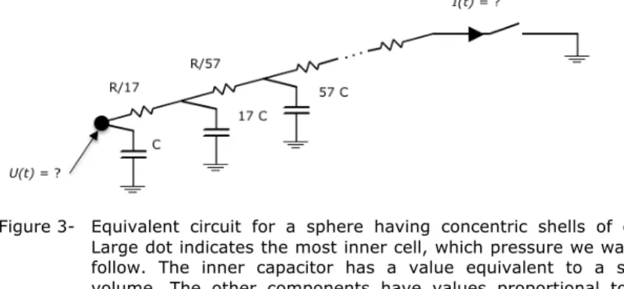
Let us consider the most inner cell of a spherical 3D array of microcavities surrounded by a shell of neighbor cells. This symmetry is depicted in Figure 2 a) and b). The first shell is surrounded by a second shell of cells and so on, until the last shell at the border. Every shell consists of an integer number of cells having the same volume. If we assume equal conductance between every two cells, then the pressure in every cell of each shell is constant and there is no flow across cells of the same shell. In other words, the flux of the exhausted gas has only radial component. Returning to the equivalent electrical circuit, all elements from the same shell are on the same potential. Therefore, we may assume that all resistors between the neighboring shells are connected in parallel due to the absence of current through the resistors with both nodes belonging to the same shell. Another consequence of this symmetry is that all capacitors from the same shell are connected in parallel to the ground. The equivalent electrical circuit is therefore dramatically simplified and now has a form presented in Figure 3.
Figure 3- Equivalent circuit for a sphere having concentric shells of cells. Large dot indicates the most inner cell, which pressure we want to follow. The inner capacitor has a value equivalent to a single volume. The other components have values proportional to the number of cells in each shell as described.
The number of volumes (capacitors) in each shell was calculated from the condition that the cell width (i.e. the shell radius increment) is as close as possible to the size of an equivalent cubic cell edge (edge=27 µm). According to this criterion, the central cell is surrounded by the first shell, which contains 17 cells; the second shell contains 57 cells, and so on. At the inner cells, this approach leads to strong shape distortion, but then quickly converges to a quasi-cubic shape with the increase of the shell radius.
3 Results and discussion
3.1 Calculation of cork pumping dynamics
The solution for 3D orthogonal arrays having 7, 15 and 23 nodes per side is graphically represented in Figure 4. Simulation was performed with the values referred in Table 1. The voltage at the inner node Uinner (or capacitor) is represented in a) and the total current Itotal is represented in b). Capacitors initial voltage (at t=0) was set to 1000 V. It should be noted that electrical initial values were chosen in order to provide a straightforward transition from voltage and current to pressure and gas flow: 1 V and 1A correspond to 1 mbar and to 1 mbar.L/s, respectively.
Regarding the voltage at the inner node, one can identify two stages: the first is a delay in which the voltage is quasi constant and a second stage when the voltage shows a clear exponential decay. The reason for the delay period is that capacitors around the inner capacitor need to be discharged before the inner one is able to feel any voltage difference and starts its discharge. The inner is this capacitor the larger will be this delay.
On the other hand, the total current shows an intense peak at time t=0 and then starts an exponential decay. The initial current peak is due to the discharge of the most external capacitors via the resistors at the borders. Once these capacitors start to be discharged, the next shell of capacitors starts to supply current and so on, until a continuous flow of charge from the inner capacitors to outside is achieved leading to an exponential decay.
Figure 4- Solution for a 3D RC array having different amount of nodes per side; a) voltage evolution at the most inner node; b) total output current.
Simulation of several cubic shapes varying the number of nodes showed that the time constant grows with the square of the number of nodes, i.e. it is proportional to the cube area.
The simulation performed with 23 nodes is far from being close to a cork stopper since it corresponds to a cube smaller than 1 mm in edge. However, the shape of the V(t) and I(t) curves are expected to be the same. The only difference is the decay rate or time constant, which will increase with the amount of nodes.
Simulation of a large amount of volumes, comparable to that of a cork stopper, can be performed only using the shell model. Its reliability was validated by comparing its results with the exact ones in the case of small 3D orthogonal arrays of microcavities. The calculations were carried out for a 3D sphere with 21 inner nodes having 13846 resistors and 4729 capacitors, which return a time constant of 3.668 s and took several hours of execution time on an ordinary PC. The simulation of the equivalent circuit using the shell model took only few seconds and return the time constant of 3.664 s confirming that both models return practically the same result. The discrepancy between the two time constants is decreasing with the number of nodes along the sphere radius, implying that it originates from the inexact description of the 3D array as a perfect sphere by an orthogonal array. The shell model is only valid for spherical shapes of 3D microcavity arrays, which does not make it suitable for modeling the pumping of cork stoppers. However, the exact calculations can be achieved for arbitrary shapes as long as their size is small in order to
1.00E+00 1.00E+01 1.00E+02 1.00E+03 1.00E+04 0 2 4 6 8 10 12 14 16 18 Uinne r (V ) Time (s) 15 nodes 23 nodes 7 nodes 1.00E+00 1.00E+01 1.00E+02 1.00E+03 1.00E+04 0 2 4 6 8 10 12 14 16 18 Itotal (A) Time (s) 15 nodes 23 nodes 7 nodes b) a)
be defined by an orthogonal array. Thus we can compare the pumping of 3D arrays having the same overall volume but different shapes. A comparison has been made between the pumping calculations of a sphere and a cylinder having the same height to diameter aspect ratio as the cork stoppers (11:6). We found that the time constant is 143.4% longer for a sphere than for the cylinder. This is as expected because in the case of a cylinder (of equal volume), the shortest distance between the inner node and the surface is smaller, having higher total conductance, which leads to a reduced time constant. In addition, it is well-known that, for a fixed volume, sphere has the smallest surface area of all shapes. Since the surface area determines the efficiency of the gas exhaust (via the total number of channels facing the vacuum), it is expected that spherical shapes should be the slowest for pumping. The factor 1.434 is independent of the volume as it was shown from calculations of systems with different sizes. Therefore, this factor can be applied to any size including that of the actual cork stopper.
At this point we have a) method to quickly calculate the pumping of a uniform spherical array of microcavities having the volume of a cork stopper and b) and a factor that can convert the previous results to the shape of a cork stopper. This enables us to estimate the pressure evolution in the center of an ideal cork stopper. A sphere having the same volume as a cork stopper (44 mm× ø24 mm) has a radius of 16.8 mm, and therefore consists of 623 shells. The solution for this circuit, corrected for the cylindrical shape, is depicted in Figure 5.
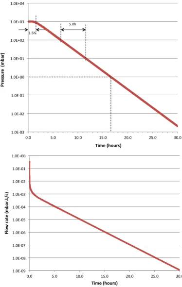
Figure 5- Simulation of 623 shells corrected for a cylinder, the equivalent of a common cork stopper. Quantities have been converted to pressure and flow in accordance to Table 1.
1.0E-03 1.0E-02 1.0E-01 1.0E+00 1.0E+01 1.0E+02 1.0E+03 1.0E+04 0.0 5.0 10.0 15.0 20.0 25.0 30.0 Pressu re ( mb ar) Time (hours) 1.5h 5.0h 1.0E-09 1.0E-08 1.0E-07 1.0E-06 1.0E-05 1.0E-04 1.0E-03 1.0E-02 1.0E-01 1.0E+00 0.0 5.0 10.0 15.0 20.0 25.0 30.0 Fl ow ra te (m ba r. L/ s) Time (hours)
Both, pressure at the inner cell and total gas flow, have the same shape as shown in the 3D orthogonal array of Figure 5Figure 5, as expected. However, now the time scale is quite different as a result of the very large time constant of 3.12 h. At the inner point, there is a delay of about 1.5 h before this point ‘begins to feel’ the pressure change in the neighboring cells. Then pressure starts to decay at a constant rate of 5 h per decade. The time to reach 1 mbar is about 16.5 h. The flow rate has an intense peak at the beginning, with a steep decrease during about 1 min, converging to the same constant decay rate as the pressure. The intense peak at start is the result of the quick depletion of all volumes close to the surface.
Simulation shown in Figure 5 is based on the values presented in Table 1. However, we should stress that those numbers are mean values of a very large and asymmetric distribution as discussed in [1]. The measured permeability for uncompressed cork could vary for about 3 orders of magnitude, which is directly reflected to the variation of conductances. Thus, real cork stoppers may behave very differently in absolute values although the shape of the pressure time curve should be preserved.
Once again, simulation of several spheres varying its diameter showed that the time constant grows with the square of the number of nodes (or radius), meaning that is proportional to its area. The same was observed for the pressure delay at the inner point (time to start the decay) that is also increasing in the same proportion.
3.2 Experimental determination of the cork stopper pumping dynamics
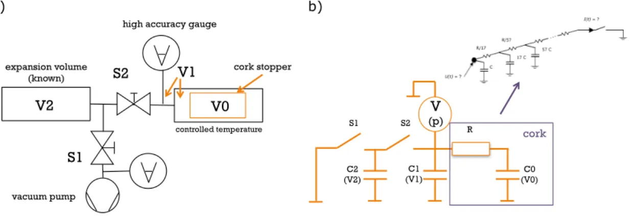
An experiment was designed to measure the time constant of a cork stopper. The experimental set-up is depicted in Figure 6 a). A first class cork stopper (mass=3.368 g,
density=148.7 kg/m3, radius= 25.2 mm and length= 45.4 mm) was placed inside a closed
container connected to an expansion container and to a vacuum pump via valves. A high accuracy gauge was fitted to the cork container to monitor pressure (1000 Torr 690A MKS Baratron). All connections and containers were made of stainless steel. The volumes were sealed with copper gaskets and tubing was sealed with metal bicones. The whole set-up was leak tested with helium to guarantee leak tightness better than 10-8 mbar.L/s.
a) b)
Figure 6- a) Experimental set-up to measure the time constant of a cork stopper. b) Electrical equivalent of the experimental set-up. Note that RC0 is indeed equivalent to a long series of resistors and capacitors in accordance with the proposed shell model (see Figure 3).
The electrical equivalent of the experimental set-up is depicted in Figure 6 b). Cork is represented by a single time constant (RC0) but should be actually described by a series of many resistors and capacitors in accordance to the shell model. After the relatively short transient regime, the pumping dynamics of the cork stopper can indeed be approximated by a single time constant, as it was shown in the previous section. We denote the replacement of the equivalent cork stopper circuit with a single resistor and capacitor as
RC approximation.
The capacitor C1 represents the dead volume (V1) around the cork, inside tubes and inside the gauge. It also includes the volume of cork defects, which are characteristic of every cork in accordance to its category (class). C2 represents the expansion volume (V2), switches are equivalent to the valves, voltmeter the pressure gauge and the common connection absolute vacuum. The conductance of the valve connecting the two chambers
high accuracy gauge
expansion volume
(known) cork stopper
vacuum pump S1 S2 V2 V1 controlled temperature V0 cork S1 S2 R C0 (V0) C1 (V1) C2 (V2) V (p)
is very big with respect to the overall conductance through which the gas flows out of the stopper, and does not therefore govern the time evolution of the pressure.
The container where the cork is placed has approximately the same volume as the expansion container. The volume of this later container was measured geometrically with low uncertainty. The dead volume (V1) was measured by placing an aluminum solid cylinder, with exactly the same dimensions of the cork stopper, and then an expansion was made. Measuring the pressure before and after the expansion, once the expansion volume is known, one can calculate the dead volume by applying the Boyle-Mariotte’s law. Figure 7 shows the expected pressure evolution after expansion by solving analytically the circuit shown in Figure 6 b) using a single RC as the cork equivalent. At start we have the initial voltage corresponding to the atmospheric pressure, and after expansion the voltage has a value p1. From its magnitude one can calculate V1 i.e. the dead volume. The volume of cork defects is the difference between the volume calculated with the solid cylinder and with the cork stopper. From the pressure at 𝑡 = ∞, pinf, we can calculate the total void volume inside the cork. At this moment, pressure inside cork and outside cork is equalized and only the dense matter of cork defines the final pressure. This can be obtained by the difference between the volume measured with the empty container and the calculated volume when the pressure converged (𝑡 = ∞) with the cork inside. In summary, a simple expansion allows us to calculate the time constant, the volume of defects in a cork stopper and the void volume of empty cells.
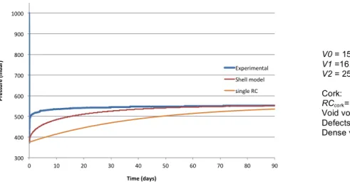
In Figure 8 is shown the result obtained for a cork stopper for 90 days. This result is compared with the result obtained from the shell model and the result from a simplistic approach i.e. the RC approximation. The shell model was applied using the values obtained experimentally for the time constant and for V1. The void volume V0 is equivalent to the sum of all capacitors in the shell model, which was also made equal to the measured V0. Therefore, the only fitting parameter was the value for R. A small resistor in series with the switch S2 was also used to avoid an infinitely high current peak at 𝑡 = 0.
The overall behavior of the measured pressure evolution is similar to that of Figure 7. However, after the expansion experiment we notice a faster approach to the final pressure, but later a very slow convergence. Although the shell model provides much closer approach than the RC approximation, the transient is still much slower than the experiment. The measured time constant of 40.66 days is about 100 times longer than the value previously predicted.
Figure 7- Expected pressure evolution after expansion taking a single RC as the cork equivalent. In the equation, R stands for the inverse of the overall equivalent flow conductance of cork.
With this pressure p1
we can calculate
V1(dead volume)
Atmospheric pressure at start in the dead volume V1 and inside cork V0
3.6E+02 4.6E+02 5.6E+02 6.6E+02 7.6E+02 8.6E+02 9.6E+02 1.1E+03 0 20 40 60 80 100 120 Pressu re Time expansion p(t) = p1+ p
(
inf− p1)
1− e −t/RV0(
)
From the final pressure pinf we can calculate V0 (total void volume inside cork) Time (days) Pr es su re (m b ar ) pinf p1
Figure 8- Pressure evolution after expansion obtained experimentally and predicted by the shell model and a single RC circuit, all having the same time constant. The main reasons for these discrepancies are twofold. First, in the shell model we assume a homogenous array of cells, all having the same volume and connected with equal channels. However, cork is a very inhomogeneous material with many natural low density defects. These defects, work as shortcuts for gas flow allowing gas to reach inner parts much faster. Therefore, describing a piece of cork as a homogenous array of cells is far from reality, or by other words, is may be a good approach only for very small pieces. The second reason is in the permeability, a quantity closely related to the vacuum conductance of plasmodesmata. As stated before, we used the mean measured permeability, but this quantity may change for several orders of magnitude. It can change not only among different cork pieces but also within the same piece of cork. Higher permeability sections will determine the gas flow in the first hours of pumping. Then, the less permeable parts will slowly be emptied by gas at a much higher time constant. Certainly, the cause for the observed difference between our model and the experiment is the combination of these two factors, somehow related. The fact that the time constant was much larger than expected, is surely related with the existence of very hermetic cells or clusters of cells where plasmodesmata are fully clogged. Gas exchange of these cells is not via the channels but through the dense wall by diffusion, which is a much slower process.
Besides the discussion of our model, it is interesting to note the ability of this experiment to get additional information highly relevant for a cork stopper. First, immediately after the expansion, we are able to obtain the volume of open defects. Since cork stoppers are classified by the amount of visible defects, the technique here described may be used to sort stoppers based in a quantitative figure, which describes the difference in volume between a ‘perfect’ stopper and a real stopper. Another relevant outcome of this experiment is the dense volume of a cork stopper. The literature, based in geometric considerations of micrographies, proposes a range between 15% and 22% in volume for cork from latecork region [6]. We got 17.8%, which perfectly matches the proposed range. We should stress that this estimation is not based on the geometric considerations revealed by electron microscopy, but in a real macroscopic measurement, although indirect. Thus, our simple experiment is a suitable technique to measure not only the amount of cork defects but also to assess the dense volume of any cork piece.
4. Conclusions
We developed a method to simulate the gas flow under molecular regime through a 3D array of microcavities. The efforts were concentrated to describe the pressure evolution in the inner point of the array and the total gas flow. Our method takes advantage of the equivalence between the gas flow and electrical current and uses readily available SPICE simulators. Although the motivation was to achieve a quantitative description of the gas evolution inside a cork stopper when subjected to vacuum, it can be applied to any 3D microcavities array or to 3D RC networks.
The limitations in size of orthogonal arrays were overcome using the so-called shell model, in which the array is described in one dimension with a series of increasing capacitors and decreasing resistors. The number of components and nodes became much less, allowing
300 400 500 600 700 800 900 1000 0 10 20 30 40 50 60 70 80 90 Pressu re ( mb ar) Time (days) Experimental Shell model single RC V0 = 15.056 cm3 V1 =16.258 cm3 V2 = 25.07 cm3 (known) Cork: RCcork= 40.66 days Void volume = 71.8% Defects volume = 10.4% Dense volume = 17.8%
us to solve very large circuits, which in 3D orthogonal arrays would require billions of components. Although this model is only valid for spherical shapes, it was extended to a cylindrical shape based in a comparison of cylindrical and spherical 3D orthogonal shapes. Our simulations are valid for molecular flow or constant conductance restrictions. However, simulations could be extended to other regimes if we replace the resistor by a specially made component having a ‘voltage’ dependent conductance.
We designed an experiment to measure the time constant of a cork stopper. The outcome of this experiment revealed much longer time constant than predicted from our shell model. However, qualitatively the result is as expected. The observed difference in the time constant should be related to the value taken for the permeability and with inhomogeneity of the cork stopper. It showed that some cork cells are extremely hermetic, releasing its gas very slowly.
The main limitation of the shell model is that it requires a homogenous media of known unit volumes and known restriction conductances. On the other hand, the observed difference can be considered as a measure of the influence of different kinds of defects on the gas flow through real cork. The discrepancy at the beginning of the experiment (too fast gas release) is an evidence of defects, which represent shortcuts for gas flow. The increased time constant at a later stage of the experiment corresponds to very hermetic cells, possibly with clogged plasmodesmata, which suppresses gas permeation through cork. Nevertheless, the model is consistent and provides reliable results once the premises are fulfilled.
Acknowledgements
Authors would like to express their gratitude for the financial support provided by Fundação para a Ciência e Tecnologia through the project UID/FIS/00068/2013.
References
1. Faria, D. P.; Fonseca, A. L.; Pereira, H.; Teodoro, O. M. N. D. Permeability of cork to gases. J. Agric. Food Chem. 2011, 59, 3590–3597.
2. Fonseca, A. L.; Brazinha, C.; Pereira, H.; Crespo, J. G.; Teodoro, O. M. N. D. Permeability of Cork for Water and Ethanol. J. Agric. Food Chem. 2013, 61, 9672– 9679.
3. Brazinha, C.; Fonseca, A. P.; Pereira, H.; Teodoro, O. M. N. D. Gas transport through cork: Modelling gas permeation based on the morphology of a natural polymer material. J. Memb. Sci. 2013, 428, 52–62.
4. Teixeira, R. T.; Pereira, H. Ultrastructural observations reveal the presence of channels between cork cells. Microsc. Microanal. 2009, 15, 539–44.
5. Teodoro, O. M. N. D.; Fonseca, A. L.; Pereira, H.; Moutinho, A. M. C. Vacuum physics applied to the transport of gases through cork. Vacuum 2014, 109, 397– 400.
6. Pereira, H., Cork: Biology, Production and Uses, Elsevier 2007, pp.40-1.
7. Hauer, V. ; Day, C. Conductance modelling of ITER vacuum systems. Fusion Engineering and Design 2009, 84, 903-907
8. Misdanitis, S; Valougeorgis, D. Design of steady-state isothermal gas distribution systems consisting of long tubes in the whole range of the Knudsen number, Journal of Vacuum Science and Technology A 2011, 29 (6), 061602,1-7
9. Roberts, Gordon W.; Sedra, Adel S. SPICE, Second Edition, The Oxford Series in Electrical and Computer Engineering, Oxford University Press, 1996.
10. Retrieved from URL https://www.analog.com/en/design-center/design-tools-and-calculators/ltspice-simulator.html, on 31/10/2018.