Finance from the NOVA – School of Business and Economics.
Resiliency and Stock Returns:
evidence from the London Stock
Exchange
Marcos António Gonçalves Cachulo Student number 26002
A Project carried out on the Master in Finance Program, under the supervision of:
André Silva
Abstract.
Literature has provided evidence of liquidity as a predictor of expected returns. However,
resiliency, as one of its dimensions, has not been extensively studied. The resiliency measure
introduced here assumes that liquidity shocks occur during the trading activity and that, in the
opening of the following day, the reversals to the new fundamental value is completed. No
significant evidence was found for a measure of resiliency that considers the trading day
return and the consecutive overnight return, both for equally-weighted and value-weighted
portfolios. Also, even considering a sample without micro-cap stocks, illiquidity premium is
not significant. (JEL: G10, G11, G12, G14)
Keywords: resiliency, liquidity, stock returns, illiquidity premium
This work used infrastructure and resources funded by Fundação para a Ciência e a
Tecnologia (UID/ECO/00124/2013, UID/ECO/00124/2019 and Social Sciences DataLab,
Project 22209), POR Lisboa (LISBOA-01-0145-FEDER-007722 and Social Sciences
1. Introduction
Traditionally, in asset pricing theory, academics have considered risk as the main key
determinant of returns. However, more recent academic papers have shown that liquidity also
a determinant of the fair value of assets. Therefore, it is worth defining what a liquid market
means. Black (1971) defined a liquid market as a continuous and efficient one where an agent
can trade securities at very near the current price. It can also be thought of as a frictionless
market where trading an appreciable quantity, in a short time period, does not make an
investor incurring in a large transaction cost and, therefore, does not create an adverse price
impact. From a firm’s perspective, liquidity is extremely correlated with the cost of capital,
and that is why it is so relevant to measure how liquid the market is. Bernstein (1987) argues
that, for a liquid market, it is necessary depth, breadth, and resiliency1. The first two
dimensions have been extensively studied in the literature, being the main methods the
Amihud’s measure and the bid-ask spread. However, surprisingly, there is not much research
about resiliency, both in defining the term and studying its implications for the overall market
liquidity. Given that fundamental values are not observable, it provides a key insight to
market participants and regulators: less resilient stocks bring greater risk attached when an
investor trades on the assumption that the current price is signalling the true value.
It was first argued by Amihud & Mendelson (1986) that, using the bid-ask spread as a
measure of liquidity, average returns observed in the market are an increasing function of
illiquidity, indicating that investors demand a premium for less liquid assets. Later, Amihud
(2002) developed an illiquidity measure as the daily ratio of absolute stock return to its dollar
volume, averaged over some period; that is, it measures the daily price impact account for a
1 Harris (2002) explains these concepts in more detail: “depth” refers to the size that investors can trade at a given price, while “breadth” refers to the price at which investors can trade a given size. For instance, “breadth” can be captured by the quote-based bid-ask spread or the trade-based effective spread, whereas “depth” can be proxied by the price impacts.
unit of trading volume. Hence, price impact could be captured with this measure. It was also
shown, in this case, that expected stock returns are an increasing function of expected
illiquidity. Given its simplicity, it has been widely used by practitioners: better measures of
illiquidity require microstructure data that may not be easily available, or may not cover long
time periods. Later research has also established a cross-sectional positive return-illiquidity
relationship (see Amihud, Mendelson, & Pedersen (2005)). These results, however, are all
US-centric. Amihud, Hameed, Kang, & Zhang (2015) were the first to provide international
evidence of illiquidity premium using Amihud’s illiquidity measure, with portfolios
composed of illiquid stocks generating significantly higher risk-adjusted returns compared to
the ones with the most liquid assets, in all the different markets.
The literature has provided some definitions of what resiliency means. Kyle (1985) refers to it
as the speed of price recovery resulting from an uninformative order-flow shock. Harris
(2002) defines it as the quickness that an asset’s price reverts to equilibrium value after large
order flow imbalances created by an uninformed trader, and that it would be guaranteed by
informed traders trying to earn profits. Therefore, in a market not perfectly liquid, an asset
would be more resilient if the price impact resulting from a liquidity shock is small, and it is
quickly repaired when a deviation occurs (see also Black (1971), Kyle (1985), Llorente,
Michaely, Saar, & Wang (2002)). Hence, resiliency could be considered as the time
dimension of liquidity. In a case where price discovery is slow, investors would demand
higher returns due to greater price uncertainty. Orders causing persistent price dislocations in
a market lacking resiliency can make the fundamental value take more time to be revealed,
resiliency measures have been suggested in recent studies2, and the empirical results have
suggested that there is, indeed, a negative relation between resiliency and stock returns.
A recent and relevant measure was presented by Hua, Peng, Schwartz, & Alan (2018), which
incorporates both the price impact of a liquidity shock and its persistence. Their resiliency
measure, denominated by RES, captures a return reversal triggered by a liquidity shock in a
not perfectly liquid market, and, with intervals properly chosen, it can be used to compare
resiliency between different stocks. Assuming that the opening half-hour is the most critical
period of the trading day, the authors described RES as the covariance between the returns of
the first thirty minutes with the remainder of the day, standardized by the daily return
variance. Therefore, a more negative RES would mean that the transitory component in the
prices after thirty minutes is larger than at the opening or closing time, indicating a higher
degree of irresiliency. Theoretically, higher values of RES would be associated with higher
expected results, and the empirical results support this idea: long-short portfolios composed
by US stocks based on RES deciles yield a nonresiliency premium ranging from 33 to 57 bps
per month for equal-weighted and value-weighted portfolios, respectively.3 Given its
simplicity, it can be easily implemented and used to compare stocks in terms of their liquidity.
However, it is worth comparing this measure with some other commonly used, namely, the
Amihud’s price impact measure and the bid-ask spread. The Amidud’s price impact measure
(Amihud, 2002) would indicate a market to be illiquid when it faces a large change in the
prices and low trading volume, even if this happens due to information efficiency that leads to
a new fundamental value. The bid-ask spread is a good measure if we are talking about small
2 See, among others, (Dong, Kempf, & Yadav, 2007), (Anand, Irvine, Puckett, & Venkataraman, 2013), and (Kempf, Mayston, & Yadav, 2011). The first defines resiliency as the mean reversion parameter of a stock’s intraday pricing-error process. The second suggests that it can be measured by the average percentage of months that trading costs exceed two-standard deviation thresholds relative to the pre-crisis period. Finally, the third defines it as the mean reversion parameter of a trading cost flow using intraday data.
3 As (Hua et al., 2018) point out, RES works best if the price adjustment finishes in the trading day, before the market closes. Otherwise, it would bias the results. There is a possibility that the best time interval depends on the characteristics of the stock and the shock.
and uncorrelated orders; however, it does not reflect the higher transaction costs suffered by
large traders (even if they split the order into several small orders) nor the impact that it
creates to the following orders. A negative externality can be created on subsequent orders by
earlier ones because of persistence (meaning that orders are somehow correlated). RES, not
only account for the price impact, but also for persistence, which makes it a better measure
than the bid-ask spread. At the same time, unlike Amihud’s one, it also differentiates better
the changes in permanent and transitory prices. Comparing these measures empirically has
suggested that RES could capture additional dimensions of liquidity.
RES relies on intraday data that are not easily accessible to practitioners and/or researchers,
and without international evidence of its significance, it looks bold to assume that it can be
applied to markets other than the US. Considering the conditions described in the main model
and the available data, this paper aims to study the effect of resiliency on expected returns as
the standardized covariance between the returns of the trading activity and the consecutive
overnight returns. This way, liquidity shocks still occur during the first period, and the second
period gives time to repair to the new fundamental value. However, there is the risk that the
transitory component has vanished by time t and that it can capture other dimensions that are
not related to liquidity. In order to test the effectiveness of this new setting, it was performed
univariate and bivariate portfolio analyses, as well as Fama-MacBeth cross-sectional
regressions. Control variables that have shown to predict future returns were included in the
analyses. No evidence was found that this new measure actually works and can be applied.
The paper proceeds as follows. Section 2 presents the resiliency measure, RES, as described
by Hua et al. (2018), as well as the modifications introduced. Section 3 describes the data, the
variables. Section 4 investigates the effect of resiliency on expected returns. Finally, the
2. Resiliency as a Measure of Liquidity
Liquidity shocks provoke movements in prices that can be decomposed on their equilibrium
and transitory components, assuming the market is not perfectly liquid. In this situation, the
transitory change takes time to disappear, and it could be argued that a more resilient market
is one with a transitory change that dissipates as quickly as possible. Given that objective of
this paper, we proceed with a brief description of the model proposed by Hua et al. (2018) and
the changes considered in this application.
2.1. The Model (Hua et al., 2018)
Consider that both liquidity and information shocks can occur in a time interval from 0, the
market’s opening, to 𝑇, the market’s closing. Moreover, the fundamental value at time 0, 𝑉 ,
equals the stock price in the opening of the market. A liquidity shock occurs at time 1 due to
an order arrival with size 𝜀 , and the impact on the transitory price is captured by 𝜅𝜎 𝜀 ,
being 𝜅 the coefficient of the price impact, 𝜎 the price volatility resulting from fundamental
information change, and 𝜀 ~𝑁(0,1). Therefore, the price impact per share can be represented
as 𝜅𝜎 . Further, the price impact is dissipated at a rate γ, 0 ≤ γ ≤ 1. Ceteris paribus, in a
resilient market, a liquidity shock leads to a small price impact (that is, a small 𝜅), which is
quickly dissipated (meaning, a small γ). At last, assume that an i.i.d. information shock,
η ~𝑁(0, 𝜎 ), affects the asset’s price. Because the goal is to focus on liquidity shocks, assume information shocks follow a random walk. Therefore,
𝑃 = 𝑉 + κ𝜎 𝜀 + η
𝑃 = 𝑉 + κ𝜎 𝜀 + η + η
(1)
At time 2, the price of the asset is analyzed so that we can understand whether the effects of
effects that these shocks create, it is necessary to set time 𝑇 to be far enough from time 2.
Hence, there is a negative relation between adjacent return 𝑃 − 𝑃 and 𝑃 − 𝑃 :
𝐶𝑜𝑣(𝑃 − 𝑃 , 𝑃 − 𝑃 ) = −𝜅 𝛾 𝜎 (2)
As defined in the introduction, our resiliency measure (RES) can be written as:
𝑅𝐸𝑆 =𝐶𝑜𝑣(𝑃 − 𝑃 , 𝑃 − 𝑃 )
𝜎 = −𝜅 𝛾 (3)
One can clearly observe that both COV and RES are negative and decreasing with respect to 𝜅
and γ. As long as price reverts to its equilibrium value by time T, both measures have
negative signals. RES cleans the effect that fundamental volatility could create on COV,
considering that expected returns are also affected by volatility in ways that are not related to
liquidity.
The selection of times t and T should be set considering that liquidity shocks occur between
time 0 and time t, while by time T reparations are completed for all stocks. However, at time t,
it should be possible to compare stocks based on their reparation levels. Based on these
conditions for a good empirical implementation, as the first thirty minutes represent the most
challenging period of a trading day activity for price discovery, the authors set the first
interval as the opening half-hour and the second as the remainer of the day.4 Thus, the second
period should allow for full recovery of the transitory prices. As a measure of fundamental
volatility, they used the daily return variance.
4 Hua et al. (2018) provide evidence of illiquidity premia for different time spans. It is presented a more general model allowing for multiple liquidity shocks and other choices of times t and T. However, it was suggested that T can be set to a point after the closing time and no test was performed.
Regarding information shocks, they may undershoot or overshoot prices, resulting in
continuations or reversals that affect RES positively or negatively.5 Thus, information shocks
and firm characteristics that may create under/overreactions were included as control
variables. Variables like analyst coverage and institutional ownership, the probability of
informed trading (Easley & O’Hara, 2004), the magnitude of earnings surprises and the event
of earnings announcement, the monthly averages of overnight returns and its absolute value
were included in the original study. Volume information was also included in their analysis
because, they argue, it could help to identify periods affected mainly by liquidity shocks from
the ones that are affected by information shocks.
2.2. Considerations about the model
Even though RES provides a simple empirical implementation, it requires a huge amount of
data that is not accessible to most investors and/or researchers. For instance, in platforms like
Bloomberg and Thomson Reuters Eikon, one can only obtain data for the last 240 days (140
days if data is downloaded) or the last 3 months, respectively. Implementing RES, as
described by the authors, in markets other than the US may not be appropriate, as there is no
evidence that it actually works. Therefore, it was decided to adapt this measure to the
available data in these platforms, and test its significance.6
As suggested by Hua et al. (2018), the model could be applied to other time periods, choosing
different t and T, as long as the conditions discussed before were met. Given the limitations of
data, the model tested in this paper considers that liquidity shocks occur between the opening
and the closing of the market (within the trading day activity), and that until the opening of
5 For instance, private information that is used for speculative trading can generate return continuations, (Llorente et al., 2002). Behavioural biases can also induce overreactions after information shocks (Daniel, Hirshleifer, & Subrahmanyam, 1998).
6 Unfortunately, there is no database similar to CRSP for other countries than the US. With such database, one could investigate this question with quality guaranteed.
the following trading day, no more liquidity shocks occur. That is, the closing price is still
affected by the shocks, and the opening price of the following day is no longer influenced by
the transitory impact. This opening price would be considered as the new fundamental value
of the stocks, meaning that all reparations have been completed by then. Therefore, our new
resiliency measure for stock i in the month m of year y is:
𝑅𝐸𝑆 =𝐶𝑜𝑣 𝑃 , − 𝑃 , , 𝑃 , − 𝑃 ,
𝜎 (4)
where 𝑃 , and 𝑃 , represent the opening and closing daily prices of month 𝑚 of year y, respectively; 𝑃 , represents the opening price of the following trading day of month m of year y; and 𝜎 the daily return variance in month m of year y.
3. Data, Variable Descriptions, and Summary Statistics
The study includes all common stocks that constituted the FTSE All-Share Index as of
November 20, 2019, which results from the aggregation of the FTSE 100, FTSE 250 and
FTSE Small Cap Indices. It represents approximately 98% of the UK market capitalization of
listed shares on the London Stock Exchange. All the data were extracted from the Bloomberg
terminal, for the time period from January 2007 to December 2017, with the exception of the
daily and monthly Fama and French data that were provided by the University of Exeter
(Gregory, Tharyan, & Christidis, 2013).7
Following the discussion in Section 1, instead of using intraday data as suggested by Hua et
al. (2018), the stock’s monthly resiliency is based on the covariance of two consecutive return
(that is, the return resulting from the trading day and the consecutive overnight return) divided
by the variance of daily returns.
Control variables are separated into two groups. The first refers to the liquidity variables,
which include the Amihud’s measure, the average bid-ask spread, the high-low spread
measure, Roll’s covariance spread, and sensitivities to Pastor & Stambaugh (2003), while the
second refers to the fundamental variables, namely the market beta from the Fama and
French, the logarithm of market capitalization, and the logarithm of the book-to-market ratio.
Moreover, the following variables were also included due to their potential to predict returns:
momentum, monthly return reversal, idiosyncratic volatility, maximum daily return, share
turnover, and long-term return volatility.
Following Amihud (2002), the illiquidity (ILLIQ) measure is the monthly average of the daily
stock’s absolute return divided by its daily dollar trading volume. The bid-ask spreads are the
monthly average of the daily quoted bid-ask spreads (SPR). Corwin & Schultz (2012)
developed a simple way to estimate spreads using the daily high and low prices (HLSPR):
𝑆 =2(𝑒 − 1) 1 + 𝑒 (5) with 𝛼 = √ − √ , 𝛽 = 𝐸 ∑ ln , and 𝛾 = ln , , , where 𝛼
represents the difference between the adjustments of a single day and a 2-day period, 𝛽 the
sum for two consecutive days of the square of the high-low log ratio, and 𝛾 the square of the
high-low log-ratio over the two days8.
Roll (1984) spread estimator is obtained by the serial covariance in price changes:
𝑆 = 2 −𝑐𝑜𝑣 ∆𝑃, , , ∆𝑃, , (6)
8 For this calculation, some assumptions were required, as suggested in the literature: observable high and low prices are required for two consecutive days, daily high is a buyer-initiated trade and daily low price is a seller-initiated trade.
where 𝑃, , is the closing price of stock 𝑖 on day 𝑑 of month 𝑚, and ∆𝑃 = 𝑃 − 𝑃 9.
Pastor & Stambaugh (2003) developed a liquidity measure for each month using daily data
within that month, and proved that innovations in liquidity also predict returns. The
sensibilities to innovations in liquidity were also included.
For the set of fundamental control variables, the market beta of individual stocks (𝐵𝐸𝑇𝐴) is
calculated following Fama & French (1992), using the previous 60 monthly returns. The
stock’s size (LNME) is the logarithm of the stock’s market capitalization (in million pounds).
The book-to-market ratio (LNBM) is also transformed in the logarithmic form.
Additionally, the momentum return (MOM) is calculated as the cumulative returns over a
period of 11 months, ending one month before the measurement month, as described in
Jegadeesh & Titman (1993). Also, in Jegadeesh (1990), monthly return reversal (REV) is
referred to as the monthly return of the previous month. The monthly idiosyncratic volatility
is obtained, as in Ang, Hodrick, Xing, & Zhang (2006), through the standard deviation of the
residuals from the Fama and French market model, estimated using daily returns10. The
maximum daily return in a month was suggested by T. G. Bali, Cakici, & Whitelaw (2010).
Share turnover (TURN) is calculated as the number of shares traded in a day divided by the
number of shares outstanding, and averaged for each month. At last, the long-term return
volatility (RET5VOL) can be described as the standard deviation of the previous 60 monthly
returns.
Summary statistics are reported, for all our variables, in Panel A of Table 1. Looking to our
variable of interest, RES, which denominates the resilience measure of stocks in a specific
month, one can observe an average monthly mean of -0.029, with a median value of -0.022,
9 When the covariance yields a positive value, most practitioners add a negative sign to the covariance. Therefore, we avoid the failure of the Roll’s model.
and a standard deviation of 0.117. Finally, the average skewness and kurtosis are -0.566 and
2.990, respectively.
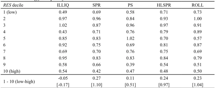
Panel B and C of Table 1 report the time-series averages of the cross-sectional Pearson
correlation coefficients; that is, the correlations are computed for each time period, and then a
time-series average is performed. Panel B refers to correlations between liquidity variables,
showing that RES is negatively correlated with ILLIQ, SPR, and HLSPR, corresponding to
-11%, -12%, and -5%, respectively. These results have the appropriate signs, and suggest that
this measure (RES) adds some value to the study of liquidity, in the sense that it captures
another dimension of liquidity. The correlations with the remaining variables can be found in
Panel C.
Fama & Macbeth (1973) methodology was also applied to test the relation between RES and
some variables, with the results available in Table 2. The outcomes suggest that there is a
positive relation between RES with highly traded and bigger stocks, and a negative relation
with liquidity (thus, suggesting a lower value of RES). Later, this methodology will also be
applied when studying the effects of RES in the expected returns.
4. Effect of RES on Expected Returns
The study of the effect of RES on expected returns was divided into three approaches, as
suggested in the original paper: univariate portfolio analysis, bivariate dependent portfolio
analysis, and Fama-MacBeth regressions. The results do not provide evidence of an illiquidity
premium between RES and 1-month forward stock returns, which will be explained in the
A. Summary statistics
Mean Median SD Skewness Kurtosis
RES -0.029 -0.022 0.117 -0.566 2.990 Liquidity variables ILLIQ 0.013 0.000 0.156 16.065 305.070 SPR(%) 0.992 0.614 1.320 4.949 61.764 PS -2.459 -0.193 105.003 -0.554 41.842 HLSPR(%) 0.566 0.518 0.405 1.081 2.235 ROLL 1.335 1.153 0.907 1.974 8.778 Firm characteristics RET 0.749 0.664 6.678 0.187 4.019 BETA 0.823 0.864 0.741 -1.214 17.486 LNME 6.836 6.687 1.638 0.436 0.889 LNBM 0.081 -0.428 1.961 0.808 0.565 MOM 1.089 1.065 0.269 1.250 8.449 REV 0.722 0.628 6.683 0.198 4.084 IVOL 1.300 1.138 0.784 2.377 13.773 MAX 3.668 3.115 2.551 3.231 25.934 TURN 0.644 0.175 5.353 19.763 425.304 RET5VOL 0.720 0.540 0.626 1.779 4.291
B. Correlations of RES and liquidity variables
RES ILLIQ SPR PS HLSPR ILLIQ -0.111 SPR -0.120 0.258 PS 0.092 0.023 0.002 HLSPR -0.051 -0.073 -0.207 -0.058 ROLL 0.026 0.069 0.118 -0.024 0.450
RET -0.013 BETA 0.060 0.009 LNME 0.118 -0.016 0.146 LNBM 0.044 -0.023 -0.102 -0.486 MOM 0.005 0.083 0.032 0.075 -0.142 REV -0.008 0.033 0.001 0.019 -0.043 0.299 IVOL 0.028 0.005 0.110 -0.266 0.203 -0.087 -0.046 MAX 0.055 0.008 0.131 -0.157 0.118 -0.074 -0.053 0.793 TURN 0.052 -0.006 0.032 0.014 0.010 -0.021 -0.010 0.070 0.056 RET5VOL 0.034 0.027 0.247 -0.229 0.190 0.052 0.026 0.601 0.518 0.065
Panel A reports the main characteristics of the variables used in this paper, namely the mean, standard deviation, skewness, and excess kurtosis. They were obtained as the time-series averages of the cross-sectional characteristics. Panels B and C report the time-series averages of the monthly cross-sectional correlations between liquidity variables and firm characteristics, respectively. Only RET is computed for 1 month forward (that is, for t+1), while the others were computed for the respective month. RES is the monthly covariance between the daily and the overnight return, scaled by the monthly variance of daily returns. BETA represents the market beta, while LNME and LNBM represent the logarithm of market capitalization and the logarithm book-to-market ratio, respectively. MOM denotes the momentum return. REV is the previous month returns. IVOL denotes the idiosyncratic volatility from the market model. MAX is the maximum daily return in a month. TURN is the average share turnover. RET5VOL is the volatility of monthly returns over the previous 5 years. These results cover the period from January 2007 to December 2017, for the full sample of 626 companies.
M1 M2 M3 M4 M5 M6 M7 TURN 0.008*** 0.007*** 0.006*** [6.47] [5.69] [4.85] LNME 0.010*** 0.009*** 0.008*** [10.68] [6.67] [5.91] SPR -0.160*** -0.057** [-4.29] [-2.13] ILLIQ -555.606*** -287.741** [-3.29] [-2.03] REV -0.000 -0.000* -0.000 [-0.81] [-1.86] [-1.51] Constant -0.032*** -0.112*** -0.012* -0.022*** -0.029*** -0.102*** -0.096*** [-7.20] [-13.38] [-1.87] [-4.57] [-6.90] [-6.72] [-6.81] N 15,708 15,312 15,708 15,708 15,708 15,312 15,312 R-sq 0.010 0.031 0.030 0.037 0.010 0.068 0.083
These results were obtained by applying the Fama & Macbeth (1973) methodology. The table presents the coefficients obtained from the time-series average of cross-sectional coefficients for some firm characteristics. N is the number of observations for each regression, and sq denotes the average R-squared of the cross-sectional regressions. Newey-West t-statistics reported in parentheses with a lag of 4. *** p<0.01, ** p<0.05, *p<0.1
4.1. Univariate Portfolio Analysis
One of the main approaches in empirical asset pricing is the univariate portfolio analysis,
where one pretends to assess the cross-sectional relation between RES and the outcome
variable, RET. The procedure is as follows: first, it is necessary to calculate the periodic
breakpoints that will be used to group the companies into portfolios based on RES, the sort
variable; then, the portfolios are formed for each time period and the average value of RET
within each portfolio for each time period is determined. Both the equally-weighted and
value-weighted average were calculated, being the market capitalization used as the weight of
value11. The primary value used to detect a cross-sectional relation between RES and RET is
the difference in averages between the highest and lowest portfolio for each time period.
11 The value-weighted approach reflects the importance of a stock relative to the rest of the market, as well as the perspective of the investor in terms of liquidity and value. However, the equally-weighted one forces both liquid and illiquid stocks to have the same weights, and the average RET may not be realized due to the high transaction costs suffered by low market cap firms.
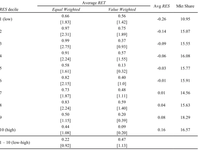
Table 3 presents the time-series averages of monthly holding returns, considering
equally-weighted and value-equally-weighted portfolios. Panel A refers to the entire sample considered since
the beginning of this analysis, while Panel B refers only to the 100 most liquid stocks (that is,
excluding the lower-cap firms)12. The average returns do not provide evidence of an
illiquidity premium, as some conditions are not met. First, in most cases, the t-statistics
calculated based on Newey & West (1987) are not strong enough to reject the hypothesis of
zero mean13. Also, the average values of RET across the deciles do not present a monotonic or
near monotonic pattern14. Therefore, there is an indication that the results of the difference
portfolios are spurious, not allowing us to infer if investors demand a premium for illiquidity
or not.15
However, if the results were significant, one could argue that resiliency is important to
large-cap stocks, given that the value-weighted difference portfolios yield a higher average return
than the equally-weighted counterparty. The lack of significance can be justified by RES
being a noisy measure of resiliency in general, and specifically to low-cap stocks with low
trading activity and higher error in measurement. Also, other effects that are correlated and
not related to liquidity can possibly be captured by our resiliency measure, affecting its
accuracy.
12 The entire sample contains all stocks composing the FTSE All-Share Index. The 100 most liquid stocks were considered those composing the FTSE 100 Index.
13 For the Newey & West (1987) t-statistics, the number of lags is an arbitrary decision. However, it was decided to use the following rule from T. Bali, Engle, & Murray (2017): the number of lags is the result of 4 / , where T is the number of periods in the time series. Therefore, with 𝑇 = 132, it was assumed a lag of 4 for the entire paper.
14 Patton & Timmermann (2010) developed a statistical test of monotonicity that could be applied. However, as it seems obvious that there is no monotonic pattern, the test was not performed. No conclusions about RES can be inferred with this condition not holding.
15 Even if the results were near to monotonicity and conclusions could be inferred, the difference portfolios “2-10” and “1-9” would not be significant, neither in Panel A nor Panel B.
Table 3 Univariate Portfolio Analysis A. Full sample
Average RET
Avg RES Mkt Share RES decile Equal Weighted Value Weighted
1 (low) 0.66 0.56 -0.26 10.95 [1.83] [1.42] 2 0.97 0.75 -0.14 15.07 [2.31] [1.89] 3 0.99 0.37 -0.09 15.55 [2.75] [0.93] 4 0.91 0.57 -0.06 16.08 [2.24] [1.55] 5 0.58 0.13 -0.03 15.77 [1.61] [0.32] 6 0.82 0.40 -0.01 15.91 [2.15] [1.0] 7 0.73 0.48 0.01 14.56 [1.87] [1.11] 8 0.83 0.59 0.04 15.63 [2.24] [1.40] 9 0.50 0.20 0.08 18.29 [1.15] [0.39] 10 (high) 0.44 0.09 0.16 16.57 [1.08] [0.20] 1 – 10 (low-high) 0.22 0.47 [0.92] [1.13] (Continued)
4.2. Bivariate Dependent Portfolio Analysis
In the previous section, only the relationship between RES and average RET was studied.
However, other effects not related to liquidity can interfere with our results, making RES to
capture them. Therefore, it is worth performing bivariate analysis and Fama-MacBeth
regression analysis.
Bivariate analysis aims to understand the relation between RES and RET, conditional on other
variables. These other variables are used as control variables, and can be separated in liquidity
and firm characteristics. The procedure applied in Table 4 is as follows: for each control
based on each tercile.16 The average return is then computed in percentage terms for the
following month. Panel A presents the results for the liquidity variables, and Panel B for the
remaining firm characteristics. As in the previous section, neither the results are monotonic or
near monotonic, nor significant. Moreover, in some situations, the difference portfolios yield
a negative value, contradicting the hypothesis.
B. FTSE 100 sample
Average RET
Avg RES Mkt Share RES decile Equal Weighted Value Weighted
1 (low) 0.93 0.66 -0.23 15.12 [2.22] [1.73] 2 0.92 0.65 -0.13 18.52 [2.08] [1.58] 3 0.91 0.53 -0.08 19.80 [2.35] [1.39] 4 0.67 0.41 -0.05 19.24 [1.52] [1.06] 5 0.58 0.27 -0.03 18.77 [1.6] [0.65] 6 0.89 0.27 -0.01 18.54 [2.51] [0.57] 7 0.82 0.56 0.02 17.81 [2.16] [1.31] 8 0.64 0.60 0.04 19.26 [1.61] [1.43] 9 0.44 0.21 0.08 20.69 [1.02] [0.45] 10 (high) 0.35 0.06 0.15 19.67 [0.86] [0.12] 1 – 10 (low-high) 0.58 0.59 [2.15] [1.49]
For each month, the breakpoints are calculated according to RES, and used to form portfolios for each time period. In these cases, the sort variable was divided into decile portfolios. The results presented are the average monthly holding period returns. Panel A refers to the full sample, while Panel B refers to the sample of the FTSE 100 components (generally assumed to be the 100 most liquid stocks traded in the United Kingdom). The column “Avg RES” reports the average RES values corresponding to each decile portfolio. The columns “Mkt Share” reports the average market share for each portfolio, assuming the last value of the month. The row “1 – 10” corresponds to the differences in monthly returns between decile 1 and decile 10 portfolios. Average returns are in percentage terms, and market share in billion pounds. Newey-West t-statistics reported in parentheses, assuming a lag of 4.
Table 4 Bivariate Dependent Portfolio Analysis A. Controlling for liquidity variables
RES decile ILLIQ SPR PS HLSPR ROLL
1 (low) 0.49 0.69 0.58 0.71 0.73 2 0.97 0.96 0.84 0.93 1.00 3 1.02 0.87 0.96 0.97 0.91 4 0.43 0.71 0.76 0.79 0.89 5 0.85 0.83 1.02 0.70 0.57 6 0.92 0.75 0.69 0.81 0.87 7 0.69 0.70 0.76 0.75 0.69 8 0.95 0.83 0.83 0.84 0.79 9 0.58 0.66 0.39 0.54 0.51 10 (high) 0.54 0.42 0.47 0.48 0.50 1 - 10 (low-high) -0.05 0.27 0.11 0.24 0.23 [-0.17] [1.10] [0.51] [0.97] [1.04] B. Controlling for firm characteristics
RES decile BETA LNME LNBM MOM REV IVOL MAX TURN RET5VOL
1 (low) 0.79 0.80 0.80 0.80 0.93 0.69 0.66 0.87 0.70 2 0.97 1.06 1.11 0.77 0.82 0.87 0.93 0.94 1.08 3 0.88 0.95 0.97 0.90 0.92 0.99 1.08 0.69 0.86 4 0.86 0.74 0.77 0.91 0.84 0.86 0.60 0.72 0.70 5 0.81 0.76 0.46 0.57 0.86 0.82 0.94 0.85 0.92 6 0.57 0.70 0.90 0.83 0.80 0.75 0.77 0.87 0.87 7 0.75 0.99 0.75 0.91 0.68 0.66 0.91 0.70 0.64 8 0.84 0.67 0.69 0.96 0.72 0.76 0.76 0.70 0.84 9 0.54 0.56 0.67 0.40 0.57 0.67 0.31 0.77 0.36 10 (high) 0.48 0.46 0.47 0.42 0.45 0.32 0.47 0.37 0.51 1 - 10 (low-high) 0.32 0.34 0.33 0.38 0.49 0.38 0.19 0.50 0.19 [1.42] [1.34] [1.36] [1.45] [2.14] [1.39] [0.80] [2.15] [0.83]
The equally-weighted average monthly returns are reported in these tables after sorting by a control variable, followed by RES. Breakpoints are first calculated for the terciles, and then, within each tercile, the decile portfolios are formed. The RES decile portfolios result from the merge between the corresponding deciles from each tercile. Panel A refers to liquidity variables (Amihud’s illiquidity ratio, bid-ask spread, Pastor-Stambaugh sensitivities to innovations, high-low spread, and Roll’s measure, respectively). Panel B refers to other variables not related to liquidity (market beta, size, book-to-market ratio, momentum, return reversal, idiosyncratic volatility, maximum daily return, share turnover, and long-term volatility). Newey-West t-statistics are reported in parentheses, with a lag of 4.
4.3. Fama-MacBeth Regressions
Finally, in order to test the effect of RES on expected returns controlling for several control
variables, the following monthly cross-sectional regression was obtained:
𝑅, = 𝛼 + 𝛾 𝑅𝐸𝑆, + 𝜑 𝑋, + 𝜀, (7)
where 𝑅, represents the excess return on stock i in month t + 1, and 𝑋, a vector of control variables for stock i in month t.
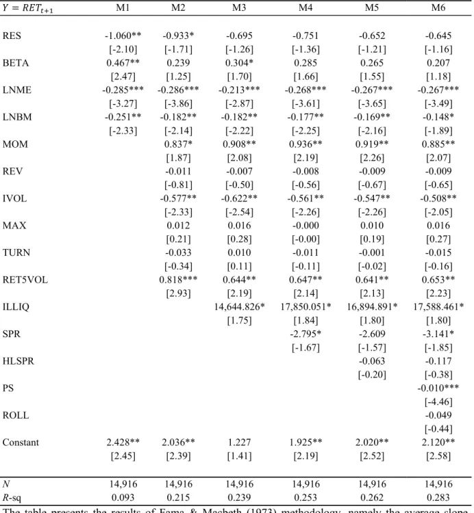
Table 5 reports the results of the Fama-MacBeth regressions above. The first model includes
the market beta, the log of market capitalization, and log of book-to-market ratio. Then, some
more control variables related to the return prediction have been included, namely, the
momentum, the monthly return reversal, the idiosyncratic volatility, the maximum daily
return, the share turnover, and the long-term monthly volatility. At last, the model was tested,
including liquidity-related variables, namely, Amihud’s illiquidity ratio, the bid-ask spread,
the high-low spread estimates, Pastor-Stambaugh sensitivities to innovations in liquidity, and
Roll’s measure. In all models, RES presents negative slopes as expected, even though they are
not significant, with the exception of model 1 with 5% and model 2 with 10% level.
Therefore, once again, there is no statistical evidence that, with our RES measure, stocks with
lower resiliency yield higher returns. However, the average slope coefficients that are
significant are in line with previous studies: LNME (stock size) is significant at 1% with
negative coefficients, consistent with (Fama & French, 1992); MOM (momentum) is positive
and significant at 10% and lower values, consistent with (Jegadeesh & Titman, 1993); REV is
negative as in (Jegadeesh, 1990), although not significant. Among the liquidity-related
variables, only ILLIQ and PS are significant at 10% and 1% level, respectively. However, one
would expect ILLIQ to be negative, which is not the case. The remaining variables do not add
Table 5 Fama-MacBeth regressions 𝑌 = 𝑅𝐸𝑇 M1 M2 M3 M4 M5 M6 RES -1.060** -0.933* -0.695 -0.751 -0.652 -0.645 [-2.10] [-1.71] [-1.26] [-1.36] [-1.21] [-1.16] BETA 0.467** 0.239 0.304* 0.285 0.265 0.207 [2.47] [1.25] [1.70] [1.66] [1.55] [1.18] LNME -0.285*** -0.286*** -0.213*** -0.268*** -0.267*** -0.267*** [-3.27] [-3.86] [-2.87] [-3.61] [-3.65] [-3.49] LNBM -0.251** -0.182** -0.182** -0.177** -0.169** -0.148* [-2.33] [-2.14] [-2.22] [-2.25] [-2.16] [-1.89] MOM 0.837* 0.908** 0.936** 0.919** 0.885** [1.87] [2.08] [2.19] [2.26] [2.07] REV -0.011 -0.007 -0.008 -0.009 -0.009 [-0.81] [-0.50] [-0.56] [-0.67] [-0.65] IVOL -0.577** -0.622** -0.561** -0.547** -0.508** [-2.33] [-2.54] [-2.26] [-2.26] [-2.05] MAX 0.012 0.016 -0.000 0.010 0.016 [0.21] [0.28] [-0.00] [0.19] [0.27] TURN -0.033 0.010 -0.011 -0.001 -0.015 [-0.34] [0.11] [-0.11] [-0.02] [-0.16] RET5VOL 0.818*** 0.644** 0.647** 0.641** 0.653** [2.93] [2.19] [2.14] [2.13] [2.23] ILLIQ 14,644.826* 17,850.051* 16,894.891* 17,588.461* [1.75] [1.84] [1.80] [1.80] SPR -2.795* -2.609 -3.141* [-1.67] [-1.57] [-1.85] HLSPR -0.063 -0.117 [-0.20] [-0.38] PS -0.010*** [-4.46] ROLL -0.049 [-0.44] Constant 2.428** 2.036** 1.227 1.925** 2.020** 2.120** [2.45] [2.39] [1.41] [2.19] [2.52] [2.58] N 14,916 14,916 14,916 14,916 14,916 14,916 R-sq 0.093 0.215 0.239 0.253 0.262 0.283
The table presents the results of Fama & Macbeth (1973) methodology, namely the average slope coefficients from the regression of monthly excess returns on RES and control variables. N stands for the number of observations, and R-sq for the average R-squared of the monthly cross-sectional regressions. Newey-West t-statistics are reported in parentheses, with a lag of 4. For details about the lagged variables, see Table 1. *** p < 0.01, ** p < 0.05, * p < 0.1
5. Conclusions
More recently, resiliency has been presented as the time dimension of liquidity. Hua et al.,
(2018) presented a resiliency measure as the standardized return covariance between the first
thirty minutes and the rest of the trading day, and that captures both the price impact of a
liquidity shock and its persistence. They find that there is a demand for illiquidity premia as
RES is negatively related to returns. Given that they only provide evidence for the US market,
one cannot use this measure outside the US without proving its effectiveness in capturing
resiliency.
As intraday data are not widely accessible for long time periods and there is no CRSP-like
database for other markets than the US, it was tested how effective was a similar measure
using the opening and closing prices in capturing the resiliency of stocks in the UK. During
the trading day, all liquidity shocks would occur, and the transitory component would still be
present, while after the closing of the market and the next opening, the shocks would have
time to completely repair from the transitory impact to the new fundamental value. The
correction from the price dislocation translates into a negative RES. These new time periods
do not contradict the conditions set by the authors of the model; however, it is obvious that it
introduces more noise into the measure, as well as it can capture other effects that can be
related to aspects other than liquidity.
Sorting stocks according to their RES levels, forming portfolios, and calculating their average
returns did not yield the required monotonic pattern as well as the significance required for
the difference portfolios. Both the equally-weighted and value-weighted portfolios reflect the
lack of monotonicity and significance. When performing double sorting in dependent way, the
results are even more inconclusive: for some control variables, besides the lack of monotonic
pattern and significance, the results of the difference portfolios are negative. Finally, the
variables, show RES to be insignificant, even though other variables are consistent with the
literature. The results are very similar for both the full and small samples.
Some explanations can be provided to justify the disastrous results obtained: first, the chosen
time periods may not be the best as it is possible that the transitory component has vanished
before time t and, therefore, it already reflects the new equilibrium price, as well as the results
may be biased due to time T not being the closing of the market, as referred by (Hua et al.,
2018); second, the quality of data is not guaranteed as it was not produced for scientific work
like CRSP database; and at last, the type of analyses performed may lead to wrong
conclusions as it makes some strong assumptions that do not reflect the reality of the data.
About the last explanation, the main issues are the failure of the assumption of linearity for
some entities with specific variables being considered (especially in the Fama-MacBeth
methodology), and the lack of joint assessment of the relation between RES and RET in the
portfolio analyses. However, it is also important to consider that there is evidence that the
Fama-French model appears to work worse for the UK than the US (see Gregory et al.,
(2013)), which can explain the insignificance of the market beta in the Fama-MacBeth
regressions performed in the last section (even though the idiosyncratic volatility has
significance). Also, the power of the Fama-MacBeth methodology has been questioned by
some researchers, as they argue that explanation power is low for small time periods, which is
the case in this paper (see Bradfield (1993)). Periods exceeding 30 years have provided more
significant results. At last, and what can be the biggest failure, is the noisy RES measure. For
future research, one can try to produce a measure that can be applied using widely accessible
References
Amihud, Y. (2002). Illiquidity and stock returns: Cross-section and time-series effects. Journal of Financial Markets, 5(1), 31–56. https://doi.org/10.1016/S1386-4181(01)00024-6
Amihud, Y., Hameed, A., Kang, W., & Zhang, H. (2015). The illiquidity premium: International evidence. Journal of Financial Economics, 117(2), 350–368. https://doi.org/10.1016/j.jfineco.2015.04.005
Amihud, Y., & Mendelson, H. (1986). Asset pricing and the bid-ask spread. Journal of Financial Economics, 17(2), 223–249. https://doi.org/10.1016/0304-405X(86)90065-6 Amihud, Y., Mendelson, H., & Pedersen, L. H. (2005). Liquidity and asset prices.
Foundations and Trends in Finance, 1(4), 269–364. https://doi.org/10.1561/0500000003 Anand, A., Irvine, P., Puckett, A., & Venkataraman, K. (2013). Institutional trading and stock
resiliency: Evidence from the 2007-2009 financial crisis. Journal of Financial Economics, 108(3), 773–797. https://doi.org/10.1016/j.jfineco.2013.01.007
Ang, A., Hodrick, R. J., Xing, Y., & Zhang, X. (2006). The Cross-Section of Volatility and
Expected Returns. The Journal of Finance, 61(1), 259–299.
https://doi.org/10.1111/j.1540-6261.2006.00836.x
Bali, T., Engle, R., & Murray, S. (2017). Empirical Asset Pricing: The Cross-Section of Stock Returns: An Overview. In Wiley StatsRef: Statistics Reference Online (pp. 1–8). https://doi.org/10.1002/9781118445112.stat07954
Bali, T. G., Cakici, N., & Whitelaw, R. F. (2010). Maxing out: Stocks as lotteries and the cross-section of expected returns $. Journal of Financial Economics, 99, 427–446. https://doi.org/10.1016/j.jfineco.2010.08.014
Bernstein, P. L. (1987). Liquidity, Stock Markets, and Market Makers. Financial Management, 16(2), 54. https://doi.org/10.2307/3666004
Black, F. (1971). Toward a Fully Automated Stock Exchange, Part I. Financial Analysts Journal, 27(4), 28–35. https://doi.org/10.2469/faj.v27.n4.28
Bradfield, D. J. (1993). An Explanation for the Weak Evidence in Support of the Systematic Risk-Return Relationship. https://doi.org/10.1007/978-3-642-46938-1_9
Corwin, S. A., & Schultz, P. (2012). A Simple Way to Estimate Bid-Ask Spreads from Daily
High and Low Prices. The Journal of Finance, 67(2), 719–760.
https://doi.org/10.1111/j.1540-6261.2012.01729.x
Daniel, K., Hirshleifer, D., & Subrahmanyam, A. (1998). Investor psychology and security market under- and overreactions. Journal of Finance, 53(6), 1839–1885. https://doi.org/10.1111/0022-1082.00077
Dong, J., Kempf, A., & Yadav, P. K. (2007). Resiliency, the Neglected Dimension of Market Liquidity: Empirical Evidence from the New York Stock Exchange. SSRN Electronic Journal. https://doi.org/10.2139/ssrn.967262
Easley, D., & O’Hara, M. (2004, August). Information and the cost of capital. Journal of Finance, Vol. 59, pp. 1553–1583. https://doi.org/10.1111/j.1540-6261.2004.00672.x Fama, EUGENE F., & French, K. R. (1992). The Cross-Section of Expected Stock Returns.
The Journal of Finance, 47(2), 427–465. https://doi.org/10.1111/j.1540-6261.1992.tb04398.x
Fama, Eugene F, & Macbeth, J. D. (1973). Risk, Return, and Equilibrium: Empirical Tests. In The Journal of Political Economy (Vol. 81).
Gregory, A., Tharyan, R., & Christidis, A. (2013). Constructing and Testing Alternative Versions of the Fama-French and Carhart Models in the UK. Journal of Business Finance & Accounting, 40(1), 306–686. https://doi.org/10.1111/jbfa.12006
Harris, L. (2002). TRADING AND EXCHANGES: Market Microstructure for Practitioners. Hua, J., Peng, L., Schwartz, R. A., & Alan, N. S. (2018). Resiliency and Stock Returns. SSRN
Electronic Journal, (646). https://doi.org/10.2139/ssrn.3218531
Jegadeesh, N. (1990). Evidence of Predictable Behavior of Security Returns. The Journal of Finance, 45(3), 881–898. https://doi.org/10.1111/j.1540-6261.1990.tb05110.x
Jegadeesh, N., & Titman, S. (1993). Returns to Buying Winners and Selling Losers: Implications for Stock Market Efficiency. In The Journal of Finance (Vol. 48).
Kempf, A., Mayston, D. L., & Yadav, P. K. (2011). Resiliency in Limit Order Book Markets:
A Dynamic View of Liquidity. SSRN Electronic Journal.
https://doi.org/10.2139/ssrn.967249
Kyle, A. S. (1985). Continuous Auctions and Insider Trading. Econometrica, 53(6), 1315. https://doi.org/10.2307/1913210
Llorente, G., Michaely, R., Saar, G., & Wang, J. (2002). Dynamic Volume-Return Relation of Individual Stocks. Review of Financial Studies, 15(4), 1005–1047. https://doi.org/10.1093/rfs/15.4.1005
Newey, W. K., & West, K. D. (1987). A Simple, Positive Semi-Definite, Heteroskedasticity, and Autocorrelation Consistent Covariance Matrix. Econometrica, 55(3), 703. https://doi.org/10.2307/1913610
Pastor, L., & Stambaugh, R. F. (2003). Liquidity risk and expected stock returns ABI/INFORM Global pg. 642. In The Journal of Political Economy (Vol. 111).
Patton, A. J., & Timmermann, A. (2010). Monotonicity in asset returns: New tests with applications to the term structure, the CAPM, and portfolio sorts. Journal of Financial Economics, 98(3), 605–625. https://doi.org/10.1016/j.jfineco.2010.06.006
Roll, R. (1984). A Simple Implicit Measure of the Effective Bid-Ask Spread in an Efficient Market. The Journal of Finance, 39(4), 1127–1139. https://doi.org/10.1111/j.1540-6261.1984.tb03897.x
Appendix
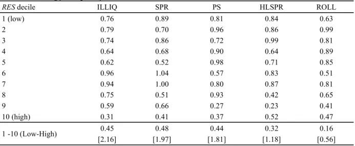
Table 6 Bivariate Dependent Portfolio Analysis (FTSE 100 sample) A. Controlling for liquidity variables
RES decile ILLIQ SPR PS HLSPR ROLL
1 (low) 0.76 0.89 0.81 0.84 0.63 2 0.79 0.70 0.96 0.86 0.99 3 0.74 0.86 0.72 0.99 0.81 4 0.64 0.68 0.90 0.64 0.89 5 0.62 0.52 0.98 0.71 0.85 6 0.96 1.04 0.57 0.83 0.51 7 0.94 1.00 0.80 0.87 0.81 8 0.75 0.51 0.93 0.42 0.65 9 0.59 0.66 0.27 0.23 0.41 10 (high) 0.31 0.41 0.37 0.52 0.47 1 -10 (Low-High) 0.45 0.48 0.44 0.32 0.16 [2.16] [1.97] [1.81] [1.18] [0.56] B. Controlling for firm characteristics
RES decile BETA LNME LNBM MOM REV IVOL MAX TURN RET5VOL 1 (low) 0.97 0.82 0.98 0.90 0.99 0.88 0.99 0.77 0.93 2 0.95 0.75 0.77 0.86 0.99 0.78 0.90 1.11 1.01 3 0.88 0.91 0.74 0.90 0.81 1.00 0.72 0.81 0.82 4 0.86 0.81 0.77 0.67 0.62 0.83 1.00 0.75 0.54 5 0.73 0.66 0.44 0.64 1.00 0.59 0.81 0.86 0.82 6 0.50 0.90 0.63 0.72 0.46 1.00 0.77 0.71 0.77 7 0.80 0.78 1.04 1.02 0.73 0.85 0.88 0.82 0.85 8 0.82 0.91 0.69 0.66 0.79 0.64 0.31 0.38 0.67 9 0.33 0.28 0.20 0.52 0.41 0.27 0.45 0.56 0.31 10 (high) 0.39 0.30 0.49 0.42 0.45 0.49 0.39 0.20 0.43 1 -10 (Low-High) 0.58 0.52 0.49 0.48 0.54 0.39 0.60 0.57 0.50 [2.11] [2.00] [1.77] [1.61] [2.01] [1.40] [2.07] [2.22] [1.85]
The equally-weighted average monthly returns are reported in these tables after sorting by a control variable, followed by RES. Breakpoints are first calculated for the terciles, and then, within each tercile, the decile portfolios are formed. The RES decile portfolios result from the merge between the corresponding deciles from each tercile. Panel A refers to liquidity variables (Amihud’s illiquidity ratio, bid-ask spread, Pastor-Stambaugh sensitivities to innovations, high-low spread, and Roll’s measure, respectively). Panel B refers to other variables not related to liquidity (market beta, size, book-to-market ratio, momentum, return reversal, idiosyncratic volatility, maximum daily return, share turnover, and long-term volatility). Newey-West t-statistics are reported in parentheses, with a lag of 4.
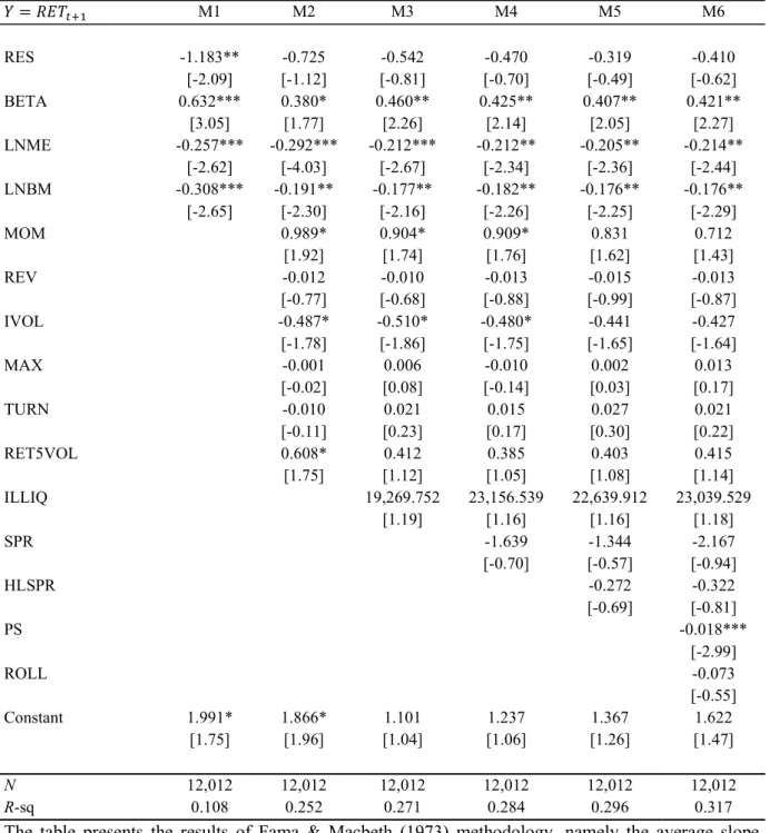
Table 7 Fama-MacBeth regressions (FTSE 100 sample) 𝑌 = 𝑅𝐸𝑇 M1 M2 M3 M4 M5 M6 RES -1.183** -0.725 -0.542 -0.470 -0.319 -0.410 [-2.09] [-1.12] [-0.81] [-0.70] [-0.49] [-0.62] BETA 0.632*** 0.380* 0.460** 0.425** 0.407** 0.421** [3.05] [1.77] [2.26] [2.14] [2.05] [2.27] LNME -0.257*** -0.292*** -0.212*** -0.212** -0.205** -0.214** [-2.62] [-4.03] [-2.67] [-2.34] [-2.36] [-2.44] LNBM -0.308*** -0.191** -0.177** -0.182** -0.176** -0.176** [-2.65] [-2.30] [-2.16] [-2.26] [-2.25] [-2.29] MOM 0.989* 0.904* 0.909* 0.831 0.712 [1.92] [1.74] [1.76] [1.62] [1.43] REV -0.012 -0.010 -0.013 -0.015 -0.013 [-0.77] [-0.68] [-0.88] [-0.99] [-0.87] IVOL -0.487* -0.510* -0.480* -0.441 -0.427 [-1.78] [-1.86] [-1.75] [-1.65] [-1.64] MAX -0.001 0.006 -0.010 0.002 0.013 [-0.02] [0.08] [-0.14] [0.03] [0.17] TURN -0.010 0.021 0.015 0.027 0.021 [-0.11] [0.23] [0.17] [0.30] [0.22] RET5VOL 0.608* 0.412 0.385 0.403 0.415 [1.75] [1.12] [1.05] [1.08] [1.14] ILLIQ 19,269.752 23,156.539 22,639.912 23,039.529 [1.19] [1.16] [1.16] [1.18] SPR -1.639 -1.344 -2.167 [-0.70] [-0.57] [-0.94] HLSPR -0.272 -0.322 [-0.69] [-0.81] PS -0.018*** [-2.99] ROLL -0.073 [-0.55] Constant 1.991* 1.866* 1.101 1.237 1.367 1.622 [1.75] [1.96] [1.04] [1.06] [1.26] [1.47] N 12,012 12,012 12,012 12,012 12,012 12,012 R-sq 0.108 0.252 0.271 0.284 0.296 0.317
The table presents the results of Fama & Macbeth (1973) methodology, namely the average slope coefficients from the regression of monthly excess returns on RES and control variables. N stands for the number of observations, and R-sq for the average R-squared of the monthly cross-sectional regressions. Newey-West t-statistics are reported in parentheses, with a lag of 4. For details about the lagged variables, see Table 1. *** p < 0.01, ** p < 0.05, * p < 0.1