Firedrake-Fluids v0.1: numerical modelling of shallow water flows using a performance-portable automated solution framework

(1)

GMDD

7, 5699–5738, 2014

Firedrake-Fluids (v0.1)

C. T. Jacobs and M. D. Piggott

Title Page

Abstract Introduction

Conclusions References

Tables Figures

◭ ◮

Back Close

Full Screen / Esc

Printer-friendly Version Interactive Discussion

Discussion

P

a

per

|

Discus

sion

P

a

per

|

Discussion

P

a

per

|

Discussion

P

a

per

|

Geosci. Model Dev. Discuss., 7, 5699–5738, 2014 www.geosci-model-dev-discuss.net/7/5699/2014/ doi:10.5194/gmdd-7-5699-2014

This discussion paper is/has been under review for the journal Geoscientific Model Development (GMD). Please refer to the corresponding final paper in GMD if available.

Firedrake-Fluids v0.1: numerical

modelling of shallow water flows using

a performance-portable automated

solution framework

C. T. Jacobs and M. D. Piggott

Department of Earth Science and Engineering, Imperial College London, London SW7 2AZ, UK

Received: 14 August 2014 – Accepted: 18 August 2014 – Published: 27 August 2014

Correspondence to: C. T. Jacobs (c.jacobs10@imperial.ac.uk)

(2)

GMDD

7, 5699–5738, 2014

Title Page

Tables Figures

◭ ◮

Back Close

Full Screen / Esc

Discussion

P

a

per

|

Discus

sion

P

a

per

|

Discussion

P

a

per

|

Discussion

P

a

per

|

Abstract

This model description paper introduces a new finite element model for the simulation of non-linear shallow water flows, called Firedrake-Fluids. Unlike traditional models that are written by hand in static, low-level programming languages such as Fortran or C, Firedrake-Fluids uses the Firedrake framework to automatically generate the model’s

5

code from a high-level abstract language called UFL. By coupling to the PyOP2 parallel unstructured mesh framework, Firedrake can then target the code in a performance-portable manner towards a desired hardware architecture to enable the efficient parallel execution of the model over an arbitrary computational mesh. The description of the model includes the governing equations, the methods employed to discretise and solve

10

the governing equations, and an outline of the automated solution process. The verifi-cation and validation of the model, performed using a set of well-defined test cases, is also presented along with a roadmap for future developments and the solution of more complex fluid dynamical systems.

1 Introduction

15

Traditional approaches to numerical model development involve the production of hand-written, low-level (e.g. C or Fortran) code for the specific set of equations that need to be solved. This task alone can be highly error-prone, often resulting in sub-optimal code, and can make the efficiency, readability and longevity of the codebase difficult to maintain (Rognes et al., 2013; Farrell et al., 2013; Mortensen et al., 2011; Maddison

20

and Farrell, 2014). Moreover, parallelisation of the code is usually accomplished by in-troducing explicit calls to parallel programming libraries such as OpenMP or CUDA. By doing so, computational scientists are frequently faced with the additional task of hav-ing to re-write their model’s code as new parallel hardware architectures and platforms emerge. At the current rate that new hardware is introduced, this development

work-25

(3)

GMDD

7, 5699–5738, 2014

Title Page

Tables Figures

◭ ◮

Back Close

Full Screen / Esc

Discussion

P

a

per

|

Discus

sion

P

a

per

|

Discussion

P

a

per

|

Discussion

P

a

per

|

be a subject/domain specialist adept in computational methods, but also well-versed in software engineering and parallelisation principles. A change to the traditional pro-gramming paradigm is clearly necessary if numerical model development is to continue in a sustainable manner.

Recent investigations into the use of automated solution techniques have shown

5

great potential in mitigating some of the issues faced with traditional approaches to writing numerical models. The FEniCS project (Logg et al., 2012) is a well-known ex-ample of a framework which uses such a solution technique to automatically generate low-level model code to solve ordinary and partial differential equations (using the fi-nite element method) from a near-mathematical high-level language, rather than by

10

hand. This hides complexity through abstraction, and allows users to focus only on the problem specification and the end results of simulations. Furthermore, optimal or near-optimal performance can be achieved through code optimisations that would be tedious to implement by hand (Ølgaard and Wells, 2010). These benefits have been realised in numerous applications in the geosciences. For example, the use of the FEniCS

frame-15

work by Maddison and Farrell (2014) allowed the runtime of their adjoint models to be as small (or even smaller) than an equivalent model generated and optimised by hand, and the extension of FEniCS by Rognes et al. (2013) to solve partial differential equations on the sphere permits ocean and atmospheric models to be written with just a few lines of high-level code rather than several thousand lines of low-level C or

For-20

tran code. Several other application areas using automated solution techniques have demonstrated similar benefits (see e.g. the works by Farrell et al., 2013; Funke and Farrell, 2014; Logg et al., 2012).

Despite the success of FEniCS, the portability of its performance across different current and future high-performance computing hardware is limited since the

gen-25

(4)

GMDD

7, 5699–5738, 2014

Title Page

Tables Figures

◭ ◮

Back Close

Full Screen / Esc

Discussion

P

a

per

|

Discus

sion

P

a

per

|

Discussion

P

a

per

|

Discussion

P

a

per

|

semi-structured nature of a three-dimensional layered mesh extruded in the vertical, as often employed in ocean/atmospheric applications), and computational operations (e.g. avoiding the re-assembly of time-independent finite element discretisation ma-trices by caching them (Maddison and Farrell, 2014)). Essentially, Firedrake provides the same high-level problem solving interface, with enhanced performance benefits.

5

Performance-portability is achieved by interfacing with the PyOP2 parallel unstructured mesh computation framework, which targets the automatically generated code towards specific high-performance computing platforms (Rathgeber et al., 2012; Markall et al., 2013). Recent application of PyOP2’s code optimisation strategies has demonstrated up to a factor 4 speed-up compared to running FEniCS-generated code (Luporini

10

et al., 2014). Furthermore, for a suite of benchmark problems (including Cahn–Hilliard, advection–diffusion and Poisson equation-based problems), Firedrake is at least as fast, if not faster, than the FEniCS framework (Rathgeber, 2014). In addition to per-formance benefits, the abstraction-based approach employed by Firedrake can also help future-proof models from hardware changes and removes a great deal of effort

15

required by computational scientists to maintain the codebase.

In light of the issues surrounding the use of static, hand-coded numerical mod-els, and the benefits that the Firedrake framework can bring, a new numerical model called Firedrake-Fluids has been developed for computational fluid dynamics (CFD)-related applications. The long-term goal of the project is to facilitate a re-engineering

20

of Fluidity (Piggott et al., 2008), another CFD package (also developed at Imperial College London) comprising hand-written Fortran code whose efficiency, readability and longevity has become challenging to maintain as the package has grown over many years. In contrast to Fluidity, Firedrake-Fluids has been written in the high-level Unified Form Language (UFL) and uses Firedrake to automate the solution process.

25

(5)

GMDD

7, 5699–5738, 2014

Title Page

Tables Figures

◭ ◮

Back Close

Full Screen / Esc

Discussion

P

a

per

|

Discus

sion

P

a

per

|

Discussion

P

a

per

|

Discussion

P

a

per

|

over submerged islands (Lloyd and Stansby, 1997), and dam breaching and flooding (Capart and Young, 1998). In addition to the core model, Firedrake-Fluids offers upwind stabilisation methods, a variety of diagnostic fields, and the Smagorinsky LES model (Smagorinsky, 1963) for the parameterisation of turbulence.

Section 2 details the set of equations that are solved and the assumptions under

5

which they are valid. Section 3 describes the numerical methods that are used to dis-cretise and solve the governing equations, followed by an overview of the automated solution techniques employed by the Firedrake framework. Section 4 presents results from a suite of test cases used to verify the correctness of the numerical model’s im-plementation, and show how well it describes the physics. A discussion regarding the

10

future developments and direction of Firedrake-Fluids is presented in Sect. 5, along with some concluding remarks in Sect. 6. Finally, Sect. “Code availability” contains in-formation regarding the availability of the Firedrake-Fluids codebase, the license under which it is released, and where the model’s documentation can be found.

2 Model equations

15

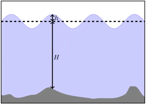
The model described in this paper solves the non-linear, non-rotational shallow water equations. These are a set of depth-averaged equations which model the dynamics of a free surface and associated depth-averaged velocities (Zhou, 2004). For modelling purposes, the free surface is split up into a mean component H and a perturbation componenth(wherehis generally assumed to be much smaller thanH) as illustrated

20

in Fig. 1.

(6)

GMDD

7, 5699–5738, 2014

Title Page

Tables Figures

◭ ◮

Back Close

Full Screen / Esc

Discussion

P

a

per

|

Discus

sion

P

a

per

|

Discussion

P

a

per

|

Discussion

P

a

per

|

2.1 Momentum equation

The momentum equation is solved in non-conservative form such that

∂u

∂t +u· ∇u=−g∇h+∇ ·T−CD

||u||u

(H+h), (1)

wheret is time, g is the acceleration due to gravity (set to 9.8 m s−2 throughout this

5

paper),u≡u(x,y) is the depth-averaged velocity, andCDis the non-dimensional drag coefficient. The stress tensorT_{is given by}

T₌_ν_∇_u₊_∇_uT₋2

3ν(∇ ·u)I, (2)

whereνis the kinematic viscosity, which is assumed to be isotropic here, andI_{is the} 10

identity tensor1.

2.2 Continuity equation

The continuity equation is given by

∂h

∂t +∇ ·((H+h)u)=0. (3)

15

3 Methods

3.1 Automated code generation

Solving a given set of equations in the Firedrake framework requires only the weak forms of the model equations (along with associated boundary and initial conditions) to

1

(7)

GMDD

7, 5699–5738, 2014

Title Page

Tables Figures

◭ ◮

Back Close

Full Screen / Esc

Discussion

P

a

per

|

Discus

sion

P

a

per

|

Discussion

P

a

per

|

Discussion

P

a

per

|

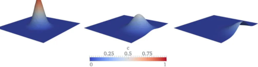
be expressed in a near-mathematical language called Unified Form Language (UFL), an embedded language that uses Python as its host (Alnæs et al., 2014). An example of a model defined in UFL which solves a two-dimensional advection–diffusion problem is given in Fig. 2 (with associated results in Fig. 3), and highlights how the implemen-tation can be accomplished with just a few lines of intuitive statements. This one file

5

containing approximately 50 lines of UFL is automatically compiled into over 600, much more complicated, lines of low-level C code which are executed over the entire mesh by PyOP2 to perform the assembly of the finite element system.

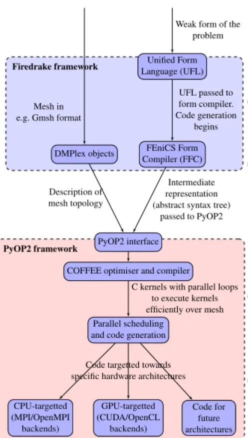
The UFL code is compiled at run-time, using a modified version of the FEniCS Form Compiler (FFC)2 (Kirby and Logg, 2006; Luporini et al., 2014), into an intermediate

10

representation as an abstract syntax tree (AST) before being passed into the PyOP2 library, as shown in Fig. 4. Furthermore, optimal numbering of the solution nodes in the domain is important to avoid cache misses and ensure efficient computation; therefore, the topology of any mesh that is provided by the user (e.g. from the Gmsh mesh gener-ator (Geuzaine and Remacle, 2009)) is described using a PETSc DMPlex object which

15

is also passed to PyOP2 along with the AST. PyOP2 then performs additional optimi-sations on the AST using the COFFEE compiler (Luporini et al., 2014) which outputs the model’s optimised low-level C code. Finally, PyOP2 calls a back-end compiler (e.g. GNU gcc or the Intel C compiler for CPUs) to compile the generated code on demand at run-time (known as just-in-time compilation), and then executes it efficiently over

20

the entire domain. As previously mentioned, in addition to targetting the code towards multi-core CPUs, PyOP2 can also target the generated code towards a specific parallel platform using, for example, the PyOpenCL and PyCUDA compilers for GPUs.

2

(8)

GMDD

7, 5699–5738, 2014

Title Page

Tables Figures

◭ ◮

Back Close

Full Screen / Esc

Discussion

P

a

per

|

Discus

sion

P

a

per

|

Discussion

P

a

per

|

Discussion

P

a

per

|

3.2 Spatial and temporal discretisation

The spatial discretisation of the model equations is performed using the Galerkin finite element method. The first step of the method involves deriving the variational/weak form of the model equations by multiplying them through by a so-called test function

w∈H1(Ω)3, where H1(Ω)3 is the first Hilbertian Sobolev space (Elman et al., 2005),

5

and integrating over the whole domain Ω; this yields, in the case of the momentum equation (Eq. 1):

Z

Ω w·∂u

∂t dV+

Z

Ω

w·(u· ∇u) dV=−

Z

Ω

gw· ∇hdV−

Z

Ω

∇w·T_dV₋

Z

Ω CDw·

||u||u

(H+h) dV. (4)

Note that the stress term has been integrated by parts and it is assumed that the normal

10

stress at all boundaries is zero. In this weak form, a solutionu∈H1(Ω)3 is sought for allw∈H1(Ω)3.

The test function and the solution u (also known as the trial function) are then re-placed by discrete representations, given by a linear combination of basis functions {φi}

N_{u_nodes}

i=1 which may be continuous or discontinuous across the cells/elements of the

15

mesh:

w=

Nu_nodes

X

i=1

φiwi, (5)

u=

N_{u_nodes}

X

i=1

φ_iu_i, (6)

whereNu_nodes is the number of velocity solution nodes in the mesh, wi are arbitrary, 20

(9)

GMDD

7, 5699–5738, 2014

Title Page

Tables Figures

◭ ◮

Back Close

Full Screen / Esc

Discussion

P

a

per

|

Discus

sion

P

a

per

|

Discussion

P

a

per

|

Discussion

P

a

per

|

represented by a (possibly different) set of basis functions{ψi} N_{h_nodes} i=1 :

h=

N_{h_nodes}

X

i=1

ψihi, (7)

whereNh_nodesis the number of free surface solution nodes, andhi are the coefficients

to be found.

5

The discrete system of size Nu_nodes×Nu_nodes for the momentum equation then becomes:

M∂u

∂t +A(u)u+Ku=−Ch+D(u,h)u, (8)

whereM, A,K,C and Dare the mass, advection, stress, gradient and drag

discreti-10

sation matrices, respectively. The notation A(u) and D(u,h) is used to highlight the non-linear dependence of the matrices on the velocity and free surface fields. A similar process is performed for the continuity equation (Eq. 3), resulting in a full block-coupled system.

The temporal discrisation is performed using the implicit backward Euler method,

15

yielding:

Mu

n+1 −un

∆t +A(u n+1

)un+1+Kun+1=−Chn+1+D(un+1,hn+1)un+1, (9)

where the superscript n represents the current time level and n+1 represents the next time level. The backward Euler method gives first-order accuracy in time. Newton

20

(10)

GMDD

7, 5699–5738, 2014

Title Page

Tables Figures

◭ ◮

Back Close

Full Screen / Esc

Discussion

P

a

per

|

Discus

sion

P

a

per

|

Discussion

P

a

per

|

Discussion

P

a

per

|

A wide variety of basis functions of arbitrary order are available through FIAT (the FInite element Automatic Tabulator) (Kirby, 2004). For the simulations presented in this paper, only the P2-P1 (i.e. piecewise-quadratic basis functions representing the veloc-ity field and piecewise-linear basis functions representing the free surface field) and P0-P1 (i.e. constant (discontinuous) basis functions for velocity and

piecewise-5

linear basis functions for the free surface) element pairs will be considered. Unless otherwise stated, the P2-P1 element pair will be used in preference to P0-P1, in order to obtain higher-order solutions.

3.3 Solution methods

Firedrake assembles the full block-coupled form of the discrete system of linear

equa-10

tions and attempts to solve it using a suite of iterative (as well as direct) numerical solution methods. Firedrake links with the PETSc library which contains a variety of linear solvers and preconditioners (Balay et al., 2006), and has proven itself in facilitat-ing geoscientific model development (Katz et al., 2007). For the simulations presented here, the GMRES linear solver (Saad and Schultz, 1986) is chosen and used in

con-15

junction with the fieldsplit preconditioner (Brown et al., 2012) which is especially suited to block-coupled systems such as the one considered here.

3.4 Setup and execution

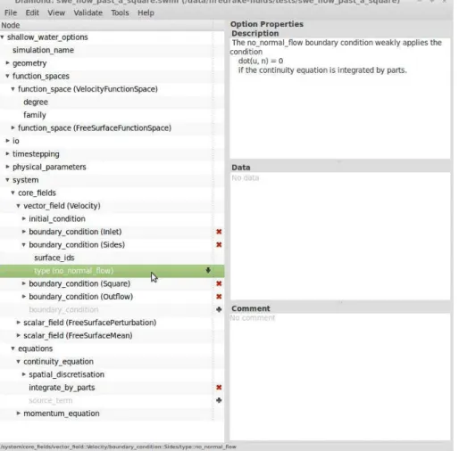
Firedrake-Fluids uses an XML-based configuration file, normally edited with the Dia-mond graphical user interface (GUI) (Ham et al., 2009), to set up simulations. Users can

20

enter options concerning the simulation’s name, the path to any input files (e.g. mesh files), the fields to be solved, discretisation options, and also the inclusion of auxiliary models such as the Smagorinsky LES model (Smagorinsky, 1963). In addition, initial and boundary conditions for each field can be specified either as a constant value, or as a C++ expression for time-varying or spatially-varying conditions. An example

(11)

GMDD

7, 5699–5738, 2014

Title Page

Tables Figures

◭ ◮

Back Close

Full Screen / Esc

Discussion

P

a

per

|

Discus

sion

P

a

per

|

Discussion

P

a

per

|

Discussion

P

a

per

|

of the GUI is shown in Fig. 5. In the case of the shallow water model, all simulation configuration files have the extension.swml (Shallow Water Markup Language).

All UFL model code is stored in themodelsdirectory of Firedrake-Fluids. Execution of, for example, the shallow water model is performed by calling the Python interpreter and providing the path to the simulation configuration file; an example for the test case

5

involving flow past a square cylinder (discussed in Sect. 4) would be:

python models/shallow_water.py tests/swe_flow_past_a_square/ swe_flow_past_a_square.swml

Solution fields are written to files in VTK format for visualisation.

10

4 Verification and validation

The following subsections describe some of the key verification and validation test cases included in Firedrake-Fluids. These tests are executed using the Buildbot au-tomated testing framework whenever a change is made to the software (Farrell et al., 2011) to ensure that any bugs introduced during the development of Firedrake-Fluids

15

(or through the development of Firedrake itself and other dependencies such as PETSc) are detected and promptly resolved by the developers.

4.1 Convergence analysis

Since no general analytical solution to the shallow water equations exists, the Method of Manufactured Solutions (MMS) (Roache, 2002) was used to perform a convergence

20

(12)

GMDD

7, 5699–5738, 2014

Title Page

Tables Figures

◭ ◮

Back Close

Full Screen / Esc

Discussion

P

a

per

|

Discus

sion

P

a

per

|

Discussion

P

a

per

|

Discussion

P

a

per

|

source term which can then be placed on the right-hand side, such that the manufac-tured/invented solution is now the analytical solution to this modified set of equations.

A two-dimensional domain with dimensions 0≤x≤1 m and 0≤y≤1 m was used for the MMS simulations. Simulations were run with three different structured meshes with characteristic element lengths∆x=0.2, 0.1 and 0.05 m. The time-steps were set

5

to ∆t=0.01, 0.005, 0.0025 s respectively, to enforce a near-constant bound on the Courant number. A zero initial condition was used for both the velocity and free surface fields, and Dirichlet boundary conditions which agreed with the analytical/manufactured solutions for the velocity and free surface were enforced along all walls of the domain.

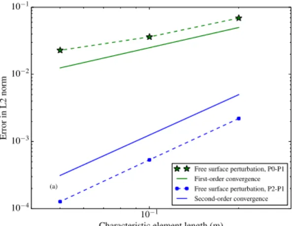
Both the P2-P1 and P0-P1 element pairs were considered. The manufactured

solu-10

tions wereh=sin(x) sin(y) and u=[cos(x) sin(y), sin(x2)+cos(y)]T. The physical pa-rameters, given in Table 1, were chosen arbitrarily and used across all the simulations. The P2-P1 element pair was first considered to check the Galerkin method with tinuous basis functions. As shown in Fig. 6a and b, this exhibited second-order con-vergence for both the velocity field and the free surface field which gave confidence in

15

the correctness of the implementation. While third-order convergence may have been expected for the velocity field because of the use of a P2 function space, the reduced order of convergence was the result of the coupling between the velocity and free sur-face fields such that the lower order of convergence in the free sursur-face field dominated. A similar effect can be seen with the P0-P1 where both the velocity and free surface

20

perturbation fields exhibited only first order convergence; it was the error in the velocity field that dominated here.

4.2 Dam failure

Dam failure (also known as dam break) problems are commonly used to test the perfor-mance of shallow water models. The presence of a discontinuity in the initial condition

25

(13)

GMDD

7, 5699–5738, 2014

Title Page

Tables Figures

◭ ◮

Back Close

Full Screen / Esc

Discussion

P

a

per

|

Discus

sion

P

a

per

|

Discussion

P

a

per

|

Discussion

P

a

per

|

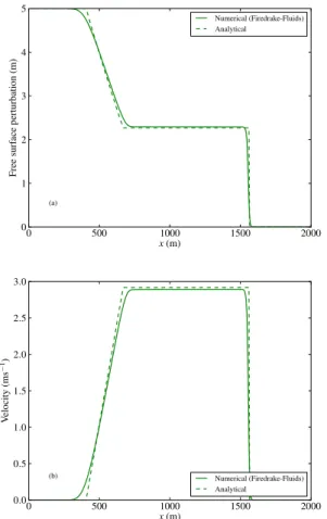
The one-dimensional case considers a channel 0≤x≤2000 m. A dam wall is lo-cated atx=1000 m which holds back the water contained in the upstream reservoir. The water in the reservoir has a total depth of 10 m, while downstream the total wa-ter depth is set to 5 m. The wawa-ter is initially at rest. Att=0 the dam is instantaneously removed, thereby simulating its failure, allowing water to rush into the downstream

sec-5

tion. Typical shock characteristics for the velocity and free surface perturbation fields were observed and compared well with the semi-analytical solutions of the correspond-ing one-dimensional Riemann problem shown in Fig. 7 att=60 s. Note that the simu-lation used an element length of∆x=5 m and a time-step of 0.25 s, as per the simula-tions of Liang et al. (2008) which consider the same scenario. The kinematic viscosity

10

was set to 1 m2s−1, and the drag coefficient was set to zero.

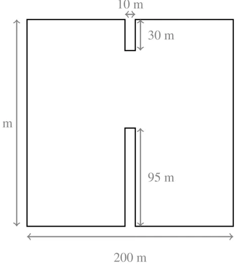
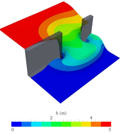
The two-dimensional case considers a square domain with dimensions 0≤x≤ 200 m and 0≤y≤200 m. A 10 m-thick dam is placed in the centre of the domain as shown in Fig. 8. In this scenario, only a partial failure of the dam is simulated; wa-ter rushes into the downstream area through a 75 m-long breach in the dam wall. As

15

before, the water is initially at rest. The upstream reservoir contains water with a to-tal height of 10 m, while the downstream section contains water with a toto-tal height of 5 m. No-normal flow boundary conditions are applied along all walls (including those of the dam). Once again, the time-step (∆t=0.2 s) and the characteristic element length (∆x=5 m) were the same as those chosen by Liang et al. (2008). The kinematic

vis-20

cosity was set to 1 m2s−1, and the drag coefficient was set to zero.

The results at t=7.2 s are shown in Fig. 9. The water that rushed into the down-stream area formed a tidal bore wave which has started to spread out laterally, while a depression/rarefaction wave has started to propagate upstream. Furthermore, small vortices are visible where the flow has separated from the dam wall immediately

down-25

(14)

GMDD

7, 5699–5738, 2014

Title Page

Tables Figures

◭ ◮

Back Close

Full Screen / Esc

Discussion

P

a

per

|

Discus

sion

P

a

per

|

Discussion

P

a

per

|

Discussion

P

a

per

|

4.3 Tidal flow over a regular bed

The test case described by Bermudez and Vazquez (1994) considers tidal flow in a one-dimensional domain of lengthL=14 000 m. The mean water height (and hence the topography of the bed) is defined by

H(x)=50.5−40x

L −10 sin

π

4x L −

1 2

. (10)

5

The initial conditionsh(x, 0)=0 andu(x, 0)=0 are applied along with the following boundary conditions for the free surface and velocity:

h(0,t)=4−4 sin

π

4t

86 400+ 1 2

, (11)

10

to simulate an incoming sinusoidally-varying tidal wave, and

u(L,t)=0, (12)

at the outflow boundary.

This simulation was performed with a mesh element length of∆x=14 m. The

time-15

step ∆t was set to 2.5 s and the simulation finished at t=9117.5 s (the same time considered by Zhou, 2004). The kinematic viscosity was set to 1 m2s−1, and the drag coefficient was set to zero. The results in Fig. 10 illustrate how the velocity of the flow increases in deeper regions of the body of water as expected. The numerical results also display good accuracy with the analytical solutions given by Bermudez and

20

Vazquez (1994), thereby further validating the numerical model.

4.4 Tidal flow over an irregular bed

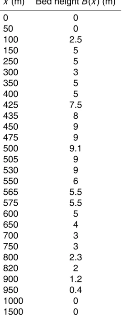
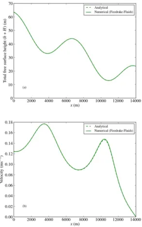
A second version of the tidal flow test case considered previously is one that involves anirregular bed topology, with sharp peaks and troughs which can be a challenge to represent accurately. This test case is described by Zhou (2004).

(15)

GMDD

7, 5699–5738, 2014

Title Page

Tables Figures

◭ ◮

Back Close

Full Screen / Esc

Discussion

P

a

per

|

Discus

sion

P

a

per

|

Discussion

P

a

per

|

Discussion

P

a

per

|

The test case considers a one-dimensional domain of lengthL=1500 m. The irregu-lar topography of the bedB(x) is defined in Table 2, and the mean water height is given byH(x)=20−B(x). The initial conditionsh(x, 0)=−4 andu(x, 0)=0 are applied along with the following boundary conditions for the free surface and velocity:

h(0,t)=−4 sin

π

4t

86 400+ 1 2

, (13)

5

u(L,t)=0, (14)

The element length∆x=7.5 m and the time-step∆t=0.3 s, as per the setup of Zhou (2004). The simulation was performed untilt=10 800 s. All remaining components of the setup were the same as the regular bed test case described in Sect. 4.3.

10

Figure 11 once again demonstrates a good match between the numerical results and the analytical solution, and demonstrates the robustness of the numerical model in accurately representing more rapidly varying areas of the solution.

4.5 Flow past a square cylinder

Simulations of laboratory-scale flow past solid objects are commonly used to

val-15

idate turbulence models due to the vast amount of available experimental data at high Reynolds numbers. In this work, the Smagorinsky LES model in Firedrake-Fluids was employed to evaluate its ability to parameterise the effects of turbulent flow past a square cylinder. The setup used in the experiments by Lyn and Rodi (1994) and Lyn et al. (1995) (and the numerical simulations by Rodi et al., 1997) was considered.

20

The dimensions of the domain are given in terms of the width/length of the square

d=0.04 m in Fig. 12. An unstructured mesh with a characteristic element length

∆x=d /15, generated with Gmsh (Geuzaine and Remacle, 2009), was used; this value of∆xis comparable to the minimum element lengths used in the numerical simulations presented in the paper by Rodi et al. (1997). The free surface mean height was set to

25

(16)

GMDD

7, 5699–5738, 2014

Title Page

Tables Figures

◭ ◮

Back Close

Full Screen / Esc

Discussion

P

a

per

|

Discus

sion

P

a

per

|

Discussion

P

a

per

|

Discussion

P

a

per

|

the fluid was set to 10−6m2s−1, which corresponded to a Reynolds number of 21 400 when using d as the length scale. The Smagorinsky LES model parameterised the turbulence via an eddy viscosity (Smagorinsky, 1963; Deardorff, 1970)

ν′=(Cs∆e) 2

|S_|. ₍₁₅₎

5

whereCsis the Smagorinsky coefficient (set to 0.164 here, within the typical range of

Cs values (Deardorff, 1971)), and ∆e is an estimate of the local mesh size which is defined here as the square root of the area of each element.|S_|_{is the modulus of the}

strain rate tensor defined by

S₌1

2

∇u+∇uT. (16)

10

This eddy viscosity, which models the dissipating effects of small-scale turbulent ed-dies on the resolved flow, is added to the physical viscosity in the stress term of the momentum equation.

Initially the velocity and free surface perturbation fields were set to zero. At the inlet,

15

a constant velocity boundary condition of 0.535 m s−1 was enforced; the inflow was laminar and no turbulent eddies were seeded along the boundary. No-normal flow boundary conditions were applied along the side walls, while no-slip boundary con-ditions were applied along all walls of the square. At the outflow, a Flather boundary condition (Flather, 1976) (specifying an external velocity equal to that at the inlet, and

20

a free surface perturbation of zero) was used to allow flow out of the domain whilst minimising reflections. A time-step of∆t=5×10−4s was chosen, and the simulation was performed untilt=15 s.

Soon after the flow began to enter the domain through the inlet, boundary layers began to form around the sides of the square where the transition to turbulence took

25

(17)

GMDD

7, 5699–5738, 2014

Title Page

Tables Figures

◭ ◮

Back Close

Full Screen / Esc

Discussion

P

a

per

|

Discus

sion

P

a

per

|

Discussion

P

a

per

|

Discussion

P

a

per

|

The stream-wise velocity along the centreline, time-averaged over a period of 15 s from the start of the simulation, was compared with the experimental data presented by Lyn et al. (1995) and Rodi et al. (1997); the results in Fig. 14 show a good match with the experimental data behind the square cylinder in the recirculating region where tur-bulent vortex shedding occurs, thereby illustrating the benefits of using the

Smagorin-5

sky LES model to accurately capture the turbulent flow characteristics. However, the wake recovery region was poorly represented; the unfortunate lack of accuracy in this region has also been observed in other numerical models (Rodi et al., 1997), and ad-ditional parameterisations and the full three-dimensionality of the problem may need to be considered to properly represent the wake.

10

5 Roadmap

The long-term aim is to extend Firedrake-Fluids into asuiteof numerical models which encompass a much wider range of flow types, as well as additional equation sets (e.g. the full Navier–Stokes equations) and constitutive equations (e.g. for describing Darcy’s law in porous media). Essentially, Firedrake-Fluids seeks to facilitate a

com-15

plete re-engineering of the Fluidity CFD code, whilst maintaining the mature modelling functionality that Fluidity offers.

One of the first application areas that Firedrake-Fluids will focus on, using the shallow water model described in this paper, is flow around tidal turbines. This will contribute to an on-going effort towards understanding the potential of renewable energy systems.

20

The multi-scale nature of the application will necessitate the use of high-performance computing, and Firedrake’s ability to target code towards more modern hardware archi-tectures such as GPU clusters will be utilised. Regarding the application area itself, the integration of adjoint optimisation models is of particular related interest. For example, recent progress in the optimisation of the layout of a tidal turbine farm using the FEniCS

25

(18)

GMDD

7, 5699–5738, 2014

Title Page

Tables Figures

◭ ◮

Back Close

Full Screen / Esc

Discussion

P

a

per

|

Discus

sion

P

a

per

|

Discussion

P

a

per

|

Discussion

P

a

per

|

library (Farrell et al., 2013) was used for this purpose. Although FEniCS and Firedrake both expect UFL statements as input, not all of the UFL interfaces are compatible with each other at present; a similar adjoint library for Firedrake (Firedrake-adjoint) is there-fore under development by the authors of DOLFIN-adjoint, and its use in the shallow water model is one of the shorter-term goals of the Firedrake-Fluids project. The issue

5

of compatibility is being addressed by the developers of Firedrake.

Realistic tidal and atmospheric modelling simulations will require boundary values to be read in from forcing files. Popular formats include NetCDF and ERA-40/GRIB, for which robust data readers will be required. Therefore, another short-term item on the roadmap is the evaluation and integration of existing readers into the Firedrake-Fluids

10

framework (or their development in-house, should no suitable reader exist).

Further to the existing Smagorinsky (1963) LES turbulence model, the roadmap fea-tures support for additional turbulence parameterisations including RANS-type models, such as those considered by Mortensen et al. (2011) for the FEniCS framework. Alter-native discretisation schemes, including control volume methods which have desirable

15

boundedness and conservativeness properties (Wilson, 2009), and high-order slope limiters for the existing discontinuous Galerkin method, will also be implemented. It is expected that a large proportion of this work will need to be undertaken within the Firedrake and PyOP2 frameworks, in addition to Firedrake-Fluids, in order to correctly describe the mesh topology (including that of the dual mesh in the case of control

20

volume methods).

6 Conclusions

This model description paper has introduced a new open-source finite element model, Firedrake-Fluids, for the simulation of shallow water flows. The model is written in the high-level, near-mathematical Unified Form Language and uses the Firedrake

frame-25

(19)

GMDD

7, 5699–5738, 2014

Title Page

Tables Figures

◭ ◮

Back Close

Full Screen / Esc

Discussion

P

a

per

|

Discus

sion

P

a

per

|

Discussion

P

a

per

|

Discussion

P

a

per

|

approach allows the focus to be on the equations that are solved and the numerical results, and removes the requirement for model developers to be experts in parallel programming and software engineering. Furthermore, the high-level specification of the problem facilitates better maintainability of the Firedrake-Fluids code base; in com-parison with the shallow water model in the Fluidity CFD code, which features static

5

hand-written Fortran, the Firedrake-Fluids source code is considerably shorter and more intuitive. Firedrake-Fluids uses approximately 400 lines (excluding comments and blank lines), compared to many thousands to perform the same task in Fluidity. Note that the 400 lines include code to obtain user settings, initial conditions, etc from the simulation configuration file, and to make the model as generic as possible; if the model

10

were to be written for a specific setup, the number of lines could potentially be further minimised to just a few dozen.

At run-time, the high-level model specification defined in Firedrake-Fluids is con-verted by Firedrake (and the PyOP2 framework) into optimised, low-level C code. This is then compiled with a back-end compiler appropriate for the target architecture (e.g.

15

the Intel compiler for CPUs, the CUDA C compiler for NVIDIA GPUs, or OpenCL for AMD GPUs). As new high-performance architectures are introduced in the future, only the PyOP2 layer which deals with code targetting needs to be modified; model devel-opers are not burdened with the task of specialising the model code itself, which is presently a common problem even in modern finite element models.

20

Several verification and validation test cases were performed to ensure the correct-ness of Firedrake-Fluids and its ability to accurately simulate physical problems. These included a convergence analysis with different finite element pairs, a simulation of dam breaching, and tidal flow dynamics over different seabed topologies. Overall, the nu-merical results were highly satisfactory and displayed good agreement with analytical

25

(20)

GMDD

7, 5699–5738, 2014

Title Page

Tables Figures

◭ ◮

Back Close

Full Screen / Esc

Discussion

P

a

per

|

Discus

sion

P

a

per

|

Discussion

P

a

per

|

Discussion

P

a

per

|

Code availability

Firedrake-Fluids is an open-source software package that has been released under the GNU General Public License (Version 3). The codebase is hosted by GitHub in a public repository and can be obtained at the following URL: https://github.com/ firedrakeproject/firedrake-fluids. The particular version of Firedrake-Fluids considered

5

in this paper (version 0.1) is available from the releases page.

Acknowledgements. This work was funded by Imperial College London. The authors acknowl-edge the use of the Imperial College High Performance Computing Service.

References

Alnæs, M. S., Logg, A., Ølgaard, K. B., Rognes, M. E., and Wells, G. N.: Unified Form

Lan-10

guage: a domain-specific language for weak formulations of partial differential equations, ACM T. Math. Software, 40, 9, doi:10.1145/2566630, 2014. 5705

Balay, S., Brown, J., Buschelman, K., Eijkhout, V., Gropp, W. D., Kaushik, D., Knepley, M. G., McInnes, L. C., Smith, B. F., and Zhang, H.: PETSc Users Manual, Tech. Rep. ANL-95/11 Revision 2.3.2., Argonne National Laboratory, 2006. 5708

15

Bermudez, A. and Vazquez, M. E.: Upwind methods for hyperbolic conservation laws with source terms, Comput. Fluids, 23, 1049–1071, doi:10.1016/0045-7930(94)90004-3, 1994. 5712, 5734, 5735

Brown, J., Knepley, M. G., May, D. A., McInnes, L. C., and Smith, B. F.: Composable Linear Solvers for Multiphysics, in: Proceeedings of the 11th International Symposium on Parallel

20

and Distributed Computing (ISPDC 2012), 55–62, doi:10.1109/ISPDC.2012.16, 2012. 5708 Capart, H. and Young, D. L.: Formation of a jump by the dam-break wave over a granular bed,

J. Fluid Mech., 372, 165–187, doi:10.1017/S0022112098002250, 1998. 5703

Deardorff, J.: A numerical study of three-dimensional turbulent channel flow at large Reynolds numbers, J. Fluid Mech., 41, 453–480, doi:10.1017/S0022112070000691, 1970. 5714

25

(21)

GMDD

7, 5699–5738, 2014

Title Page

Tables Figures

◭ ◮

Back Close

Full Screen / Esc

Discussion

P

a

per

|

Discus

sion

P

a

per

|

Discussion

P

a

per

|

Discussion

P

a

per

|

Divett, T., Vennell, R., and Stevens, C.: Optimization of multiple turbine arrays in a channel with tidally reversing flow by numerical modelling with adaptive mesh, Philos. T. R. Soc. A, 371, 1471–2962, doi:10.1098/rsta.2012.0251, 2013. 5702

Elman, H. C., Silvester, D. J., and Wathen, A. J.: Finite Elements and Fast Iterative Solvers: with Applications in Incompressible Fluid Dynamics, Oxford University Press, 2005. 5706

5

Farrell, P. E., Piggott, M. D., Gorman, G. J., Ham, D. A., Wilson, C. R., and Bond, T. M.: Au-tomated continuous verification for numerical simulation, Geosci. Model Dev., 4, 435–449, doi:10.5194/gmd-4-435-2011, 2011. 5709

Farrell, P. E., Ham, D. A., Funke, S. W., and Rognes, M. E.: Automated derivation of the ad-joint of high-level transient finite element programs, SIAM J. Sci. Comput., 35, C369–C393,

10

doi:10.1137/120873558, 2013. 5700, 5701, 5716

Flather, R. A.: A tidal model of the northwest European continental shelf, Memoires de la So-ciété Royale des Sciences de Liège, 10, 141–164, 1976. 5714

Funke, S. W. and Farrell, P. E.: A framework for automated PDE-constrained optimisation, ACM T. Math. Software, submitted, 2014. 5701

15

Funke, S. W., Farrell, P. E., and Piggott, M. D.: Tidal turbine array optimisation using the ad-joint approach, Renew. Energ., 63, 658–673, doi:10.1016/j.renene.2013.09.031, 2014. 5702, 5715

Geuzaine, C. and Remacle, J.-F.: Gmsh: a 3-D finite element mesh generator with built-in pre- and post-processing facilities, Int. J. Numer. Meth. Eng., 79, 1309–1331,

20

doi:10.1002/nme.2579, 2009. 5705, 5713

Ham, D. A., Farrell, P. E., Gorman, G. J., Maddison, J. R., Wilson, C. R., Kramer, S. C., Ship-ton, J., Collins, G. S., Cotter, C. J., and Piggott, M. D.: Spud 1.0: generalising and au-tomating the user interfaces of scientific computer models, Geosci. Model Dev., 2, 33–42, doi:10.5194/gmd-2-33-2009, 2009. 5708, 5729

25

Hill, J., Collins, G. S., Avdis, A., Kramer, S. C., and Piggott, M. D.: How does multiscale mod-elling and inclusion of realistic palaeobathymetry affect numerical simulation of the Storegga Slide tsunami, Ocean Model., in press, 2014. 5702

Imperial College London: The Firedrake Project, available at: http://firedrakeproject.org/ (last access: 14 August 2014), 2013. 5701

30

(22)

GMDD

7, 5699–5738, 2014

Title Page

Tables Figures

◭ ◮

Back Close

Full Screen / Esc

Discussion

P

a

per

|

Discus

sion

P

a

per

|

Discussion

P

a

per

|

Discussion

P

a

per

|

Kirby, R. C.: Algorithm 839: FIAT, a new paradigm for computing finite element basis functions, ACM T. Math. Software, 30, 502–516, doi:10.1145/1039813.1039820, 2004. 5708

Kirby, R. C. and Logg, A.: A compiler for variational forms, ACM T. Math. Software, 32, 417–444, doi:10.1145/1163641.1163644, 2006. 5705

Kramer, S. C., Piggott, M. D., Hill, J., Kregting, L., Pritchard, D., and Elsaesser, B.: The

mod-5

elling of tidal turbine farms using multi-scale, unstructured mesh models, in: Proceedings of the 2nd International Conference on Environmental Interactions of Marine Renewable En-ergy Technologies, (EIMR2014), Stornoway, Scotland, 2014. 5702

Liang, S.-J., Tang, J.-H., and Wu, M.-S.: Solution of shallow-water equations using least-squares finite-element method, Acta Mech. Sinica, 24, 523–532,

doi:10.1007/s10409-008-10

0151-4, 2008. 5711

Lloyd, P. M. and Stansby, P. K.: Shallow-water flow around model conical islands of small side slope. II: Submerged, J. Hydraul. Eng., 123, 1068–1077, doi:10.1061/(ASCE)0733-9429(1997)123:12(1068), 1997. 5703

Logg, A. and Wells, G. N.: DOLFIN: Automated finite element computing, ACM T. Math.

Soft-15

ware, 37, ISSN: 0098-3500, doi:10.1145/1731022.1731030, 2010. 5705

Logg, A., Mardal, K.-A., Wells, G. N., et al.: Automated Solution of Differential Equations by the Finite Element Method, Springer, doi:10.1007/978-3-642-23099-8, 2012. 5701

Luporini, F., Varbanescu, A. L., Rathgeber, F., Bercea, G.-T., Ramanujam, J., Ham, D. A., and Kelly, P. H. J.: COFFEE: an optimizing compiler for finite element local assembly, ACM T.

20

Archit. Code Op., submitted, 2014. 5702, 5705

Lyn, D. A. and Rodi, W.: The flapping shear layer formed by flow separation from the forward corner of a square cylinder, J. Fluid Mech., 267, 353–376, doi:10.1017/S0022112094001217, 1994. 5713

Lyn, D. A., Einav, S., Rodi, W., and Park, J.-H.: A laser-Doppler velocimetry study of

ensemble-25

averaged characteristics of the turbulent near wake of a square cylinder, J. Fluid Mech., 304, 285–319, doi:10.1017/S0022112095004435, 1995. 5713, 5715

Maddison, J. R. and Farrell, P. E.: Rapid development and adjoining of transient finite el-ement models, Comput. Method. Appl. M., 276, 95–121, doi:10.1016/j.cma.2014.03.010, 2014. 5700, 5701, 5702

30

(23)

GMDD

7, 5699–5738, 2014

Title Page

Tables Figures

◭ ◮

Back Close

Full Screen / Esc

Discussion

P

a

per

|

Discus

sion

P

a

per

|

Discussion

P

a

per

|

Discussion

P

a

per

|

28th International Supercomputing Conference, ISC, Vol. 7905 of Lecture Notes in Computer Science, Springer, 279–289, 2013. 5702

Martin-Short, R., Hill, J., Kramer, S. C., Avdis, A., Allison, P. A., and Piggott, M. D.: Tidal re-source extraction in the Pentland Firth, UK: potential impacts on flow regime and sediment transport in the Inner Sound of Stroma, Renew. Energ., submitted, 2014. 5702

5

Mingham, C. G. and Causon, D. M.: High-Resolution Finite-Volume Method for Shallow Wa-ter Flows, J. Hydraul. Eng., 124, 605–614, doi:10.1061/(ASCE)0733-9429(1998)124:6(605), 1998. 5711

Mortensen, M., Langtangen, H. P., and Wells, G. N.: A FEniCS-based programming framework for modeling turbulent flow by the Reynolds-averaged Navier–Stokes equations, Adv. Water

10

Resour., 34, 1082–1101, doi:10.1016/j.advwatres.2011.02.013, 2011. 5700, 5716

Ølgaard, K. B. and Wells, G. N.: Optimisations for quadrature representations of finite element tensors through automated code generation, ACM T. Math. Software, 37, ISSN: 0098-3500, doi:10.1145/1644001.1644009, 2010. 5701

Piggott, M. D., Gorman, G. J., Pain, C. C., Allison, P. A., Candy, A. S., Martin, B. T.,

15

and Wells, M. R.: A new computational framework for multi-scale ocean modelling based on adapting unstructured meshes, Int. J. Numer. Meth. Fl., 56, 1003–1015, doi:10.1002/fld.1663, 2008. 5702

Rathgeber, F.: Productive and Efficient Computational Science Through Domain-specific Ab-stractions, Ph.D. thesis, Imperial College London, submitted, 2014. 5702, 5728

20

Rathgeber, F., Markall, G. R., Mitchell, L., Loriant, N., Ham, D. A., Bertolli, C., and Kelly, P. H.: PyOP2: a high-level framework for performance-portable simulations on unstructured meshes, in: High Performance Computing, Networking Storage and Analysis, SC Compan-ion, IEEE Computer Society, 1116–1123, 2012. 5702

Roache, P. J.: Code verification by the method of manufactured solutions, J. Fluid. Eng.-T.

25

ASME, 124, 4–10, doi:10.1115/1.1436090, 2002. 5709

Rodi, W., Ferziger, J. H., Breuer, M., and Porquié, M.: Status of large Eddy simulation: results of a workshop, Trans. ASME, 119, 248–262, 1997. 5713, 5715

Rognes, M. E., Ham, D. A., Cotter, C. J., and McRae, A. T. T.: Automating the solution of PDEs on the sphere and other manifolds in FEniCS 1.2, Geosci. Model Dev., 6, 2099–2119,

30

(24)

GMDD

7, 5699–5738, 2014

Title Page

Tables Figures

◭ ◮

Back Close

Full Screen / Esc

Discussion

P

a

per

|

Discus

sion

P

a

per

|

Discussion

P

a

per

|

Discussion

P

a

per

|

Saad, Y. and Schultz, M. H.: GMRES: A generalized minimal residual algorithm for solving nonsymmetric linear systems, SIAM J. Sci. Stat. Comp., 7, 856–869, doi:10.1137/0907058, 1986. 5708

Smagorinsky, J.: General circulation experiments with the primitive equations, Mon. Weather Rev., 91, 99–164, doi:10.1175/1520-0493(1963)091<0099:GCEWTP>2.3.CO;2,

5

1963. 5703, 5708, 5714, 5716

Trangenstein, J. A.: Numerical Solution of Hyperbolic Partial Differential Equations, Cambridge University Press, 2009. 5731

Wilson, C.: Modelling Multiple-Material Flows on Adaptive Unstructured Meshes, Ph.D. thesis, Imperial College London, 2009. 5716

10

(25)

GMDD

7, 5699–5738, 2014

Title Page

Tables Figures

◭ ◮

Back Close

Full Screen / Esc

Discussion

P

a

per

|

Discus

sion

P

a

per

|

Discussion

P

a

per

|

Discussion

P

a

per

|

Table 1.Parameters used in the MMS test cases.

Parameter Description Value

CD Drag coefficient 0.0025

ν Kinematic viscosity 0.6 m2s−1

(26)

GMDD

7, 5699–5738, 2014

Title Page

Tables Figures

◭ ◮

Back Close

Full Screen / Esc

Discussion

P

a

per

|

Discus

sion

P

a

per

|

Discussion

P

a

per

|

Discussion

P

a

per

|

Table 2.Bed heights along the seabed from Zhou (2004).

x(m) Bed heightB(x) (m)

0 0

50 0

100 2.5

150 5

250 5

300 3

350 5

400 5

425 7.5

435 8

450 9

475 9

500 9.1

505 9

530 9

550 6

565 5.5

575 5.5

600 5

650 4

700 3

750 3

800 2.3

820 2

900 1.2

950 0.4

1000 0

(27)

GMDD

7, 5699–5738, 2014

Title Page

Tables Figures

◭ ◮

Back Close

Full Screen / Esc

Discussion

P

a

per

|

Discus

sion

P

a

per

|

Discussion

P

a

per

|

Discussion

P

a

per

|

H

h

(28)

GMDD

7, 5699–5738, 2014

Title Page

Tables Figures

◭ ◮

Back Close

Full Screen / Esc

Discussion

P

a

per

|

Discus

sion

P

a

per

|

Discussion

P

a

per

|

Discussion

P

a

per

|

(29)

GMDD

7, 5699–5738, 2014

Title Page

Tables Figures

◭ ◮

Back Close

Full Screen / Esc

Discussion

P

a

per

|

Discus

sion

P

a

per

|

Discussion

P

a

per

|

Discussion

P

a

per

|

(30)

GMDD

7, 5699–5738, 2014

Title Page

Tables Figures

◭ ◮

Back Close

Full Screen / Esc

Discussion

P

a

per

|

Discus

sion

P

a

per

|

Discussion

P

a

per

|

Discussion

P

a

per

|

Firedrake framework

PyOP2 framework

Unified Form Language (UFL)

FEniCS Form Compiler (FFC) DMPlex objects

PyOP2 interface

Weak form of the problem

UFL passed to form compiler. Code generation

begins Mesh in

e.g. Gmsh format

Description of mesh topology

COFFEE optimiser and compiler

Parallel scheduling and code generation

CPU-targetted (MPI/OpenMPI backends)

GPU-targetted (CUDA/OpenCL

backends)

Code for future architectures Intermediate representation (abstract syntax tree)

passed to PyOP2

C kernels with parallel loops to execute kernels efficiently over mesh

Code targetted towards specific hardware architectures

220

225

230

235

(31)

GMDD

7, 5699–5738, 2014

Title Page

Tables Figures

◭ ◮

Back Close

Full Screen / Esc

Discussion

P

a

per

|

Discus

sion

P

a

per

|

Discussion

P

a

per

|

Discussion

P

a

per

|

(32)

GMDD

7, 5699–5738, 2014

Title Page

Tables Figures

◭ ◮

Back Close

Full Screen / Esc

Discussion

P

a

per

|

Discus

sion

P

a

per

|

Discussion

P

a

per

|

Discussion

P

a

per

|

10−1

Characteristic element length (m) 10−4

10−3

10−2

10−1

E

rr

or

in

L

2

nor

m

Free surface perturbation, P0-P1 First-order convergence Free surface perturbation, P2-P1 Second-order convergence (a)

10−1

Characteristic element length (m) 10−5

10−4

10−3

10−2

10−1

E

rr

or

in

L

2

nor

m

Velocity (x-component), P0-P1 Velocity (y-component), P0-P1 First-order convergence Velocity (x-component), P2-P1 Velocity (y-component), P2-P1 Second-order convergence (b)

(33)

GMDD

7, 5699–5738, 2014

Title Page

Tables Figures

◭ ◮

Back Close

Full Screen / Esc

Discussion

P

a

per

|

Discus

sion

P

a

per

|

Discussion

P

a

per

|

Discussion

P

a

per

|

0 500 1000 1500 2000

x(m) 0

1 2 3 4 5

F

re

e

sur

fa

ce

pe

rt

ur

ba

ti

on

(m

)

Numerical (Firedrake-Fluids) Analytical

(a)

0 500 1000 1500 2000

x(m) 0.0

0.5

1.0

1.5

2.0

2.5

3.0

V

el

oc

it

y

(m

s

−

1)

Numerical (Firedrake-Fluids) Analytical

(b)

(34)

GMDD

7, 5699–5738, 2014

Title Page

Tables Figures

◭ ◮

Back Close

Full Screen / Esc

Discussion

P

a

per

|

Discus

sion

P

a

per

|

Discussion

P

a

per

|

Discussion

P

a

per

|

200 m

10 m

30 m

95 m

(35)

GMDD

7, 5699–5738, 2014

Title Page

Tables Figures

◭ ◮

Back Close

Full Screen / Esc

Discussion

P

a

per

|

Discus

sion

P

a

per

|

Discussion

P

a

per

|

Discussion

P

a

per

|

(36)

GMDD

7, 5699–5738, 2014

Title Page

Tables Figures

◭ ◮

Back Close

Full Screen / Esc

Discussion

P

a

per

|

Discus

sion

P

a

per

|

Discussion

P

a

per

|

Discussion

P

a

per

|

(37)

GMDD

7, 5699–5738, 2014

Title Page

Tables Figures

◭ ◮

Back Close

Full Screen / Esc

Discussion

P

a

per

|

Discus

sion

P

a

per

|

Discussion

P

a

per

|

Discussion

P

a

per

|

(38)

GMDD

7, 5699–5738, 2014

Title Page

Tables Figures

◭ ◮

Back Close

Full Screen / Esc

Discussion

P

a

per

|

Discus

sion

P

a

per

|

Discussion

P

a

per

|

Discussion

P

a

per

|

x

y

14 _d

4 _.

5 _d

_d

19 _.

5 _d

(39)

GMDD

7, 5699–5738, 2014

Title Page

Tables Figures

◭ ◮

Back Close

Full Screen / Esc

Discussion

P

a

per

|

Discus

sion

P

a

per

|

Discussion

P

a

per

|

Discussion

P

a

per

|

(40)

GMDD

7, 5699–5738, 2014

Title Page

Tables Figures

◭ ◮

Back Close

Full Screen / Esc

Discussion

P

a

per

|

Discus

sion

P

a

per

|

Discussion

P

a

per

|

Discussion

P

a

per

|