BEM NUMERIC SIMULATION OF SPILLWAY FLOWS WITH
DISCONTINUOUS LINEAR ELEMENTS
Carlos E. F. Mello*and José P. S. Azevedo†
*
Department of Civil Engineering – School of Mines Federal University of Ouro Preto
Campus Morro do Cruzeiro, s/n, Zip code 35400-000, Ouro Preto, MG, Brazil e-mail: [email protected]
†
Computational Hydraulics Laboratory - Department of Civil Engineering COPPE - Federal University of Rio de Janeiro
Postbox 68506, Zip code 21945-970, Rio de Janeiro, RJ, Brazil
Key words: Free Surface Flow, Spillway, Boundary Element Method, Iterative Procedure.
1 INTRODUCTION
The application of numeric methods in water resources engineering is increasing more and more and in an accelerated way. In many cases, these techniques provide cheap and efficient alternatives for projects’ verification and optimization, helping engineers to diagnose and solve possible problems.
Several water resources problems can be represented by the potential theory, such as sluice gates or spillways flows, examples of rapidly varied free surface flows governed by gravity. This kind of flow presents inherent difficulties for its solution. The difficulties, as pointed out by von Karman1, arise not only from the nonlinear character of the dynamic boundary condition on the free surface, but also from the fact that the position of this surface is not known a priori. Since flows of this nature are characterized by highly curved contours, it is usually necessary, for a good numeric approach, the use of refined mesh or high order interpolation functions. Besides, due to the intrinsic nonlinearity of the problem, a great number of iterations seems to be inevitable in the solution procedure. Thus, the efficiency of the solution method is important and can become the main factor in the choice of the numeric method.
According to Cheng et al.2, serious numeric solutions to free surface flows began with Southwell & Vaisey3, using the finite difference method (FDM) with handmade calculations. Other finite difference solutions include those by McNown et al.4, Cassidy5 and, more recently, Liao et al.6 that combined FDM with a coordinate system that follows the contour. Solutions with the finite element method (FEM) began with McCorquodale & Li7 for sluice gates. Among many other works that appeared in the literature using FEM, it can be mentioned Ikegawa & Washizu8, Isaacs9, Betts10, Khan & Steffler11, Sankaranarayanan & Rao12. As examples of use of the boundary element method (BEM) in the solution of this problem type, it can be mentioned Cheng et al.2, Liggett & Salmon13, Jovanovic14 and Medina et al.15. Other adopted technique is the jointly use of complex function theory and integral equations solved numerically, as in the works of Merino16, Vanden-Broeck17 and Guo et al.18. Recently, the finite volume method (FVM) has also been used, as in the works of Olsen & Kjellesvig19, Unami et al.20 and Song & Zhou21.
This work presents the numeric simulation of spillways flows through BEM classic formulation with discontinuous linear elements, having as basis the procedure proposed by Cheng et al.2.
2 BASIC FORMULATION
In the spillway flow problem here treated, only the irrotational steady state is considered. The stream function ψ formulation in a domain Ω is used and the governing differential equation is the Laplace’s equation:
0 y x ) x
( 2 2
2 2
2 =
∂ ∂ + ∂ ∂ =
where x = (x,y) is a generic point of the domain. Both the fixed boundaries and the free surface are streamlines, therefore the value of ψ should be constant, that is:
boundary fixed
the on 0
=
ψ (2)
surface free the on q
=
ψ (3)
being q the flow rate per unit width. On the free surface the dynamic boundary condition (Bernoulli’s theorem) requires (Figure 1):
0 p p , B h g
2 atm 2
= = =
+
ν (4)
where ν is the velocity; g is the acceleration of gravity; h is the free surface elevation measured from an arbitrary datum; B is the constant of Bernoulli; and p is the pressure.
Figure1: General Outline of the spillway
Starting from the stream function definition, the following relationship in the free surface is valid:
n
∂ ∂ = ψ
ν (5)
being n the unit normal from the free surface. Substituting equation (5) in (4) gives:
B h n g 2
1 2+ =
∂
∂ψ on the free surface (6)
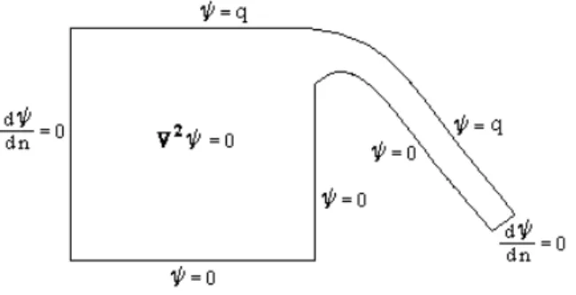
For the purpose of limiting a domain for the numeric solution, it is made a cut, at right angles to the primary velocity, at a certain distance upstream and downstream the spillway crest. On the cut sections the following boundary condition is applied:
0
= ∂ ∂ n
ψ (7)
which means that there is no normal velocity to the main flow. This condition, although approximate, is applied sufficiently far away from the spillway crest that is quite accurate and any small error that occurs doesn't affect the interesting part of the flow (Cheng et al.2). Figure 2 shows the boundary conditions on the problem domain.
Figure 2: Domain and boundary conditions
A short description of BEM classic formulation used to solve equation (1) with essential (equations 2 and 3) and natural boundary conditions(equation 7) is presented in the following section.
3 BEM CLASSIC FORMULATION
BEM consists of transforming a differential equation and boundary conditions that govern a certain problem in a boundary integral equation, being one way the use of the concept of weighted residuals (Brebbia et al.22).
The integral equation that represents the equation (1) and your boundary conditions (2), (3) and (7), and that allows the calculation of unknowns ψ and ν at the boundary and in the domain, can be written in the following form (Brebbia et al.22):
) x ( d ) x ; ( ) x ( ) x ( d ) x ; ( ) x ( ) ( ) (
c = * Γ − * Γ
∫
∫
Γν ψ ξ Γψ ν ξξ ψ
ξ (8)
The function ψ*
domain Ω* that contains Ω. The points ξ and x are denominated, respectively, source and field point. The function ν*
(ξ;x) is the normal derivative of *
ψ (ξ; x) on the boundary. Equation (8) involves two fields: one that is known ( *
ψ ,ν*
) corresponding to the solution of a unit point source in an infinite domain; and other for which we want to obtain the solution (ψ,ν) corresponding to the boundary conditions of the problem in the domain Ω. In two dimensions we have:
= r 1 ln 2 1 ) x ; ( * π ξ ψ (9) n r 2 1 n ) x ; ( * * ∂ ∂ − = ∂ ∂ = σ π ψ ξ ν (10)
where r is the distance between the source ξ and the field x points; and σ is the unit vector from ξ to x direction.
Equation (8) is valid for internal points ξ or belonging to the boundary Γ since it is observed that: Ω ∈ Γ ∈ Γ ∪ Ω ∉ = ξ ξ π β ξ ξ se 1 se 2 ) ( se 0 ) ( c (11)
where β is the internal angle at the point ξ. If the boundary is smooth at ξ, β = π e c(ξ) = 0,5.
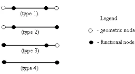
3.1 Boundary discretization
The original boundary Γ is replaced by a finite number of linear boundary elements. There are basically two types of linear elements: the continuous ones, where the functional nodes coincide with the geometric nodes (extreme points of the element); and the discontinuous ones, where at least one of the functional nodes is located inside the element. Figure 3 illustrates all the possible types:
Figure 3: Types of linear elements
The whole BEM discretization process and numeric approach to solve equation (1) with boundary conditions of Dirichlet type (equations 2 and 3) and Neumann type (equation 7), which leads to a linear algebraic equations system of unknowns ψ and ν at the boundary functional nodes, are described in full detail in Mello et al.23.
4 SOLUTION PROCEDURE
The inclusion of the free surface dynamic boundary condition (equation 6) brings complications for the solution of the problem. This aspect is treated here in much the same way as it has been done for most of the finite difference and finite element solutions. That is, for problems with a known flow rate, q, a position of the free surface boundary is adopted and the problem solved from equations (1), (2), (3) and (7). The Bernoulli constant is then calculated on the free surface by equation (6). If B is the same for all free surface points (nodes), the problem is solved. Otherwise, the adopted free surface is adjusted, iteratively, in order that the value of B becomes constant at all points. A similar procedure can be used for problems with a known Bernoulli constant, B. A position of the free surface is assumed and the problem is solved from equations (1), (2), (6) and (7). The flow rate, q (equation 3), is part of the solution. If q is constant for all free surface points, the problem is solved. Otherwise, an iterative process should be used to adjust the free surface elevation. The method of adjusting the free surface is problem dependent (Cheng et al.2).
{ }
{ }
Bdh dB dh dB dh dB h
T 1 T
∆ ∆
=
− (12)
being {∆h} the elevation adjustment vector only for the real free surface nodes; {∆B} is the departure of the Bernoulli constant for each free surface node (real and pseudo) from its objective value. For a given iteration k+1, the objective value of B is taken to be the average value of iteration k. The matrix [dB/dh] is computed by displacing, in turn, each real free surface node a small distance ∆h from its adopted value (or the result of the previous iteration) and computing the variation in the Bernoulli constant at all free surface nodes, real and pseudo. This calculation requires a complete solution for each real free surface node, and the BEM does it in a quite efficient way. As a practical matter, a step factor (or damping factor), which controls the stability and the rate of convergence, is adopted in order that the adjustments to the free surface are always reasonable. Therefore, the values of the elevation in the iteration k+1 are obtained by the following equation:
{ }
k1{ }
k{ }
kh h
h + = +α ∆ (13)
where α is the step parameter. The value of this parameter is problem dependent and should be determined empirically. The solution is considered satisfactory when the calculated corrections on the free surface elevation become sufficiently small.
5 RESULTS
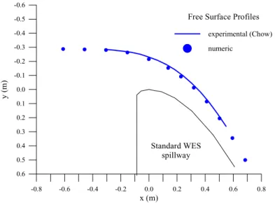
In order to verify the efficiency of the developed procedure, some examples were simulated and the numeric results of one of them are presented. The chosen example is a standard WES type spillway designed for a flow rate q = 0.3744 m3/s/m and a height P = 1.52 m. This example allows validate the implemented formulation, since it has known experimental results (Chow24).
The domain was limited upstream to a distance (3.05 m) of twice the spillway height and downstream to a distance (1.16 m) in which the parament almost equaled the reservoir's bottom level. The domain discretization was made by 54 linear elements being 24 for the free surface. Discontinuous elements were used to considered the two values of the velocity ν in all the real corners.
Table 1: Main adopted parameters
Parameter Value Number of Gauss quadrature points to numeric integration 4 Tolerance to end iterative process (permitted maximum error) (m) 0.00015 Step factor α 0.1 Displacement ∆h to numeric calculation of matrix [dB/dh] (m) 0.0762 Number of pseudo-nodes per element (NPN) on the free surface 4
Table 2: Main computed parameters
Parameter Value Number of iterations 59 Average B on the free surface (m) 0.30448 Spillway discharge coeficient C = q / B1,5 2.228 Critical section position – coordinate x (m) 0.00343 Critical deep (m) 0.20943
-0.8 -0.6 -0.4 -0.2 0.0 0.2 0.4 0.6 0.8 x (m)
-0.6
-0.5
-0.4
-0.3
-0.2
-0.1
0.0
0.1
0.2
0.3
0.4
0.5
0.6
y (m
)
Free Surface Profiles
experimental (Chow) numeric
Standard WES spillway
Figure 4: Comparison of experimental and numeric free surface profiles
In relation to the data presented in Table 1 it is worth to point out the following observations:
value along the whole procedure, this led to a slower convergence and a greater number of iterations. According to Jovanovic14, an automatic adjustment of this parameter at each iteration, through gradient type methods, would improve the rate of convergence.
The value of the displacement ∆h to the numeric calculation of matrix [dB/dh] also has great influence in the success and efficiency of the iterative process. Very small values of ∆h tend to increase the instability. It was adopted the same value of ∆h for all free surface points and matrix [dB/dh] was calculated only once, in the beginning of the process, to become it more computationally efficient. According to Cheng et al.2, since matrix [dB/dh] changes little from one iteration to the next, it is not necessary to recalculate it each time. When it does have to be recomputed, it is necessary only to disturb and recompute those points in and near the uncertainty zone. As it is not clear when is necessary to update the matrix, it is suggested a more detailed study to optimize this procedure. Another possible change is the adoption of different values of the displacement ∆h for each point, for instance, proportional to the difference between the value of the constant B in the point and an objective or average value of B.
The number of pseudo nodes has certain importance, since in the case of linear elements, its absence generates instability. According to Liggett & Salmon13, the use of cubic splines elements eliminates the need of pseudo nodes. The procedure here developed allows the option of 2 up to 9 pseudo nodes per element on the free surface, and was verified that starting from the value 4, no significant improvement of the results were found.
Now in relation to the data presented in Table 2 it can be detached the following aspects: The number of 59 iterations, for the circumstances commented previously, can be considered a good result. Cheng et al.2 don't comment on this value in their work and Jovanovic14 reports a number of iterations about 160.
The value of the computed discharge coefficient, equal to 2.228, was very close to the experimental value 2.225 (Chow24). This represents an error of only 0.13%. Cheng et al.2 obtained an error of 0.50% and Jovanovic14 maximum mistakes about 3%.
The procedure also allows at its end the determination of the critical section by interpolation, since the value of the Froude number is calculated continually at all free surface points.
In relation to Figure 4, it can be noticed a good adherence among the numeric results and the experimental profile (Chow24), just occurring a small discrepancy in the area of greater curvature, having BEM underestimated a little the surface water profile, what means that the calculated velocities were a little larger. This can be associated to the fact that the mathematical model supposes that there are no energy losses along the flow over the spillway.
5. CONCLUSIONS
The iterative procedure for the Newton-Raphson method adopted, and proposed by Cheng et al.2, led to very good results, but it still presents a slow convergence in the zone of uncertainty, taking a high number of iterations.
The role of the step parameter α, as well as the value of the displacement ∆h to the numeric calculation of matrix [dB/dh] should be more investigated to be achieved an improvement on the rate of convergence of the iterative process.
6 REFERENCES
[1] T. Von Karman, “The Engineer grapples with non-linear problems”, Bulletin of the Mathematics Society, 46, 615-683, (1940).
[2] A.H.-D. Cheng, J.A. Liggett and P.L-F. Liu, “Boundary calculations of sluice and spillway flows”, Journal of the Hydraulics Division – ASCE, 107, no. HY10, 1163-1178, (1981).
[3] R.V. Southwell and G. Vaisey, “Relaxation methods applied to engineering problems: XIII, Fluid motions characterized by free streamlines”, Philosophical Transactions, Royal Society of London, Series A, 240, 117-161, (1946).
[4] J.S. McNown, E-Y. Hsu and C-S. Yih, “Application of the relaxation technique in fluid mechanics”, Transactions – ASCE, 120, 650-686, (1955).
[5] J.J. Cassidy, “Irrotational flow over spillways of finite height”, Journal of the Engineering Mechanics Division – ASCE, 91, no. EM6, 155-173, (1965).
[6] H. Liao, W. Xu and C. Wu, “Residual pressure feedback method for simulation of free surface flow”, Journal of Hydraulic Engineering, 124, no. 10, 1049-1052, (1998). [7] J.A. McCorquodale and C.Y. Li, “Finite element analysis of sluice gate flow”,
Engineering Journal, 54, no. 3, 1-4, (1971).
[8] M. Ikegawa and K. Washizu, “Finite element method applied to analysis of flow over a spillway crest”, InternationalJournal for Numerical Methods in Engineering, 6, 179-189, (1973).
[9] L.T. Isaacs, “Numerical solution for flow under sluice gates”, Journal of the Hydraulics Division – ASCE, 103, no. HY5, 473-481, (1977).
[10] P.L. Betts, “A variational principle in terms of stream function for free-surface flows and its application to the finite element method”, Computers and Fluids, 7, 145-153, (1979). [11] A.A. Khan and P.M. Steffler, “Modeling overfalls using vertically averaged and moment
equations”, Journal of Hydraulic Engineering, 122, no. 7, 397-402, (1996).
[12] S. Sankaranarayanan and H.S. Rao, “Finite element analysis of free surface flow through gates”, International Journal for Numerical Methods in Fluids, 22, 375-392, (1996). [13] J.A. Liggett and J.R. Salmon, “Cubic spline boundary elements”, International Journal
for Numerical Methods in Engineering, 17, 543-556, (1981).
hydrodinamic calculations”, International Journal for Numerical Methods in Fluids, 12, 835-857, (1991).
[16] F. Merino, “Fluid flow through a vertical slot under gravity”, Applied Mathematical Modelling, 20, 934-939, (1996).
[17] J.-M. Vanden-Broeck, “Numerical calculations of the free-surface flow under a sluice gate”, Journal of Fluid Mechanics, 330, 339-347, (1997).
[18] Y. Guo et al., “Numerical modelling of spillway flow with free drop and initially unknown discharge”, Journal of Hydraulic Research, 36, no. 10, 785-801, (1998). [19] N.R.B. Olsen and H.M. Kjellesvig, “Three-dimensional numerical flow modelling for
estimation of spillway capacity”, Journal of Hydraulic Research, 36, no. 5, 775-784, (1998).
[20] K. Unami et al., “Two-dimensional numerical model of spillway flow”, Journal of Hydraulic Engineering, 125, no. 4, 369-375, (1999).
[21] C.C.S. Song and F.Y. Zhou, “Simulation of free surface flow over spillway”, Journal of Hydraulic Engineering, 125, no. 9, 959-967, (1999).
[22] C.A. Brebbia, J.C.F. Telles and L.C Wrobel, Boundary Element Techniques: Theory and Applications in Engineering, Springer-Verlag, Berlin, (1984).
[23] C.E.F. Mello et al., “Computational implementation of the classic and hypersingular formulations of the boundary element method for 2D potential problems with discontinuous linear elements”, In: Proc. of the 20th Iberian Latin-American Congress on Computational Methods in Engineering (XX CILAMCE), São Paulo/SP, (CD-ROM), (1999) (in portuguese).