Flavio Maldonado Bentes*
Fundação Jorge Duprat Figueiredo de Segurança e Medicina do Trabalho
Rio de Janeiro/RJ – Brazil
Jules Ghislain Slama
Instituto Alberto Luiz Coimbra de Pós-Graduação e Pesquisa em Engenharia Rio de Janeiro/RJ – Brazil
*author for correspondence
Sensitivity analysis of airport
noise using computer simulation
Abstract: This paper presents the method to analyze the sensitivity of airport noise using computer simulation with the aid of Integrated Noise Model 7.0. The technique serves to support the selection of alternatives to better control aircraft noise, since it helps identify which areas of the noise curves experienced greater variation from changes in aircraft movements at a particular airport.
Keywords: Sensitivity analysis, airport noise, computer simulation.
LIST OF SYMBOLS
ANAC: National Civil Aviation Agency
Scxi: Sensitivity coficient of the movement variable Scxi’: Sensitivity coeficient of the movement variable
without 10% of the aircrafts
dB: Decibel
dB(A): Decibel, according to the A ponderation curve
DNL: Day-night average noise level
ΔΦ: Variation in the area of the noise curve FAA: Federal Aviation Administration
Φ: Area of the noise curve INM: Integrated Noise Model
LAeq: Equivalent sound pressure level
LAeqD: Day equivalent sound pressure level
LAeqN: Night equivalent sound pressure level RBAC: Brazilian Regulation for Civil Aviation
SEL: Sound exposure level
Sxi: Sensitivity to a movement xi
SBRF: Guararapes International Airport (Recife/PE – Brazil)
xi: Movement Variable for a group of aircrafts
InTrOducTIOn
With the global growth of aerial navigation, airport authorities have become more concerned about issues
related to aircraft noise. For Infraero (2010), to navigate
means to safely conduct a watercraft or an aircraft from one point to another, which is a complex guidance
process that enables long journeys with the goal to reach a speciic place safely. The safety aspect should
also include issues related to sound emission, once they
can cause not only discomfort, but also damage to those
who are continuously exposed to this type of noise. It is
possible to say that the study of airport noise is really
relevant worldwide, especially regarding issues related to aircraft noise. As to this aspect, the study concerning
the sensitivity analysis is signiicantly helpful, since it
allows identifying which areas of the noise curves have varied more from the changes in the aircraft movements
at a speciic airport.
Airport noise is usually a result of discreet events, such as landings and take-offs. There are different noise sources in airports, coming from land operations involving aircraft fueling, movements and maintenance, however, landing and take-off operations are considered as the main noise sources of an airport. According to Morais, Slama and Mansur (2008), airport noise is a result of a sound field with intermittent temporal characteristics. The noise coming from the aircraft movements is directly related to the
procedures of the aircrafts on the ground, be it before
take-off or after landing. The study concerning airport
noise embraces different fields of knowledge, from
physics to mechanical engineering, especially focusing on the acoustic phenomenon and issues concerning the environment.
The sensitivity analysis of airport noise is a method that uses acoustics software to simulate scenarios,
with the objective to help control airport noise. Together with the guidelines of the balanced approach established by the International Civil Aviation Organization (2004), the technique contributes with a Received: 25/06/11
Accepted: 09/09/11
better analysis of the variations in the areas exposed
to the levels of noise coming from the aircrafts. The numerical simulations use the Integrated Noise Model
7.0 (INM), which was created by the Federal Aviation Administration (2009) and enables the appearance
of airport noise curves. INM requires the description of different airport parameters, such as runways,
trajectories, fleet, route, airport coordinates, runway
thresholds and noise curves starting from the choice of discomfort metrics.
METrIcS FOr AIrPOrT nOISE
There are different types of metrics to assess airport noise. Basically, noise metrics represents the energetic average of
sound pressure levels in a deinite period of time. According
to the Brazilian Regulation for Civil Aviation 161 (2011),
in order to determine noise curves, calculations should be
made with software that uses appropriate methods with the day-night average level (DNL). This study presents a summary of some existing metrics: equivalent sound pressure level – Laeq, sound exposure level – SEL, and day-night average level – DNL).
Equivalent sound pressure level - Laeq
Noise levels can usually vary during a deinite period
of time. For Gerges (2000), the damaging effects of
noise depend not only on its level, but also on how long it lasts. It is possible to say that Laeqis a constant sound pressure level that is equal to the variable noise levels
during the measuring period, in terms of acoustic energy. As a consequence, Laeqrepresents the average sound level resulting from the integration throughout a period of time
that can be deined with the logarithmic sum of all sound
levels. Laeqcan be divided between day and night. LaeqDis the day equivalent sound pressure level and represents the average sound energy calculated during daytime, from 7 to 22h, with a total of 15 hours. LaeqDis determined by Eq. 1.
LAeqD = 10log 1
54000 7
22
10
LA(t) 10 (t)dt
µ
¬ ® ¼ ¾ ½ (1)LAeqN is the night equivalent sound pressure level, and represents the average sound energy calculated during the night, from 22h to 7h, with a total of 9 hours. LaeqNis
determined by Eq. 2.
LAeqN = 10log 1
32400 22
7
10
LA(t) 10 (t)dt
µ
¬ ® ¼ ¾ ½ (2)Sound exposure level – SEL
SEL represents the total noise energy produced from
an event. It is possible to say that SEL represents a logarithmic expression of the acoustic energy of the
event, once it exceeds a speciic type of noise, as if it
had happened within a second. Thus, SEL is obtained by
the sum of all sound pressure levels in one unit of time, inside the analyzed interval. Since SEL is a logarithmic
expression regarding sound exposure in time, it can be
used to compare the noise energy of events that last for different periods. The mathematical formulation
to express the deinition of SEL is demonstrated in Eq. 3:
SEL = 10log 1
T0 t tT P2
A
P02(t)dt
µ
¬ ® ¼ ¾ ½ ½ (3)day-night Average Sound Level – dnL
DNL is commonly used to deine the level of exposure
to airport noise, and it also corresponds to the average
sound energy caused by all airport events in a period
of 24 hours. Ten dB (A) are added to the noise level for sound levels that occur during the night, from 22h to 7h of the next day, due to the higher sensitivity and
disturbances caused by noise at night. According to the
Code of Federal Regulations 14 CFR 150 (2004), DNL
combines the sound energy of all aircraft operations
from events that occur during daytime at an average
noise exposure for that day. It is possible to say that the
calculation of DNL is similar to Laeq, except that DNL adds 10 dB (A) to the night sound and is calculated in a period of 24 hours. According to Bistafa (2006), the
relation between them is obtained with Laeq of every
hour of each day. The average energy sum of the day and night, with extra 10 dB (A), results in the DNL.
Eq. 4 mathematically deines DNL.
DNL = 10log 1 3600.24 ¯ ° ± 7 22 10 LA(t) 10 dt + 7
22 10
LA(t)10
10 dt
µ
µ
¬ ® ¼ ¾ ½ ½ ¿ À Á (4)DNL is usually used to deine the areas of the noise
curve, and has functions such as quantifying the cumulative noise exposure, considering events taking
METHOdS And dATA
With the use of INM 7.0, the variations of the area of the noise curve (Δφ) will be studied with DNL, as established
by RBAC 161 (2011), in relation with variations of airport movements. The values of sensitivity coeficients are calculated after the elaboration of noise curves with
INM, over the individual variation of each parameter,
with other ixed parameters. Thus, it is possible to say that
K = (x1,x2,...,xn), in which the variable xn corresponds to the aircraft movements, during the daytime or the night. Considering the φ variation when x1, x2,..., xn varies to
x1 + ∆x1, x2 + ∆x2,…, xn + ∆xn,as demonstrated in Eq. 5:
¨Kx1x2,...,xn"Kx1+¨x1,x2+¨x2
,...,
xn+¨xn- Kx1x2,...,xn
)
(5)Thus, Δφcan be described as demonstrated in Eq. 6:
¨Kx1,x2,...,xn"K¨x1
x1 ¨x2
K
x2 ¨xn K
x2 (6)
Therefore, it is possible to obtain the relative variation,
which is equivalent to Eq. 7:
"
¨x1 x1
K
x1
¨Kx1,x2,...,xn x1
Kx1,x2,...,xn Kx1,x2,...,xn
¨xn xn
K
xn xn
Kx1,x2,...,xn (7)
The xi motion sensitivity can be deined by Eq. 8:
K
x1 xi
Sxi=Kx
1,x2,...,xn (8)
Replacing Eq. 8 in Eq. 7, we come to Eq. 9:
"Sx1¨x1Sx2 Sxn
x1
¨x2 x2
¨Kx1,x2,...,xn
Kx1,x2,...,xn
¨xn
xn (9)
The values of sensitivity coeficients are deined from
the determination of areas of noise curve using INM for the variation of each xi movement. Thus, φ values were determined for x1, x2, x3, (…), xn in the initial situation and after the parameter variation for x1 + Δx1,x2 + Δx2,x3 +
Δx3,(…), xn+ Δxn. Therefore, the sensitivity coeficient for xi will be demonstrated in Eq. 10:
~
CSxi xi ¨K ¨[i
K (10)
The sensitivity coeficients can be expressed for x1
movements (group A, daytime), x2 (group A, night), x3
(group B, daytime), and x4 (group B, night). Equation 11
represents the sensitivity coeficient for a determinate xi
movement:
~
CSxi -10 Ki - K0
K0 (11)
Considering a logarithmic relation, it is possible to
relate the logarithm of the area of the noise curve and
the logarithm in relation to the movements multiplied by their respective sensitivity coeficients, which will result
in Eq. 12:
logeKx1x2,...,xn"CSx1
log
ex
1+CSx2log
ex
2 +...+ CSxn
log
ex
n+ cte
(12)The sensitivity analysis was conducted with computational numerical analysis in Guararapes International Airport – Recife/PE, Brazil (SBRF). Information concerning the
lights was gathered via online airline schedule provided by the National Civil Aviation Agency (ANAC), from Brazil (2011). Table 1 presents aircraft movements by
period.
rESuLTS
The areas of noise curves were calculated for all the aircrafts. Afterwards, the areas of noise curves in groups A
and B were calculated both for daytime (D) and night (N)
Movements Period Aircrafts Group
x1 D A318, A319, A320, A321, A332, A343, B733, B734, B737, B738, B744, B752, B762, B763, E190, F100
A
x2 N A318, A319, A320, A321, A332, A343, B733, B734, B737, B738, B744, B752, B762, B763, E190, F100
A
x3 D AT72, B722, L410 B
x4 N AT72, B722, L410 B
dnL (dB(A))
noise curve areas with all the aircrafts (km²) All the aircrafts Group A
daytime (x1)
Group A night (x2)
Group B daytime (x3)
Group B night (x4)
55 47,609 11,382 30,998 3,875 1,778
60 19,034 4,359 11,753 1,326 0.527
65 7,030 1,684 4,582 0.338 0.111
70 2,569 0.589 1,756 0.102 0.045
75 1,022 0.161 0.689 0.023 0.014
80 0.25 0.065 0.173 0 0.001
85 0.1 0.013 0.073 0 0
Table 2. Values of noise curve areas with all the aircrafts.
dnL (dB(A))
noise curve areas after 10% of the aircrafts were removed (km²) All the aircrafts Group A
daytime (x1’)
Group A night (x2’)
Group B daytime (x3’)
Group B night (x4’)
55 38,983 10,513 28,028 3,685 1,617
60 14,266 4,166 10,699 1,289 0.556
65 5,645 1,581 4,313 0.479 0.214
70 2,025 0.579 1,648 0.165 0.087
75 0.838 0.231 0.653 0.045 0.028
80 0.197 0.086 0.258 0.008 0.005
85 0.085 0.023 0.095 0.001 0
Table 3. Values of noise curve areas after 10% of the aircrafts were removed.
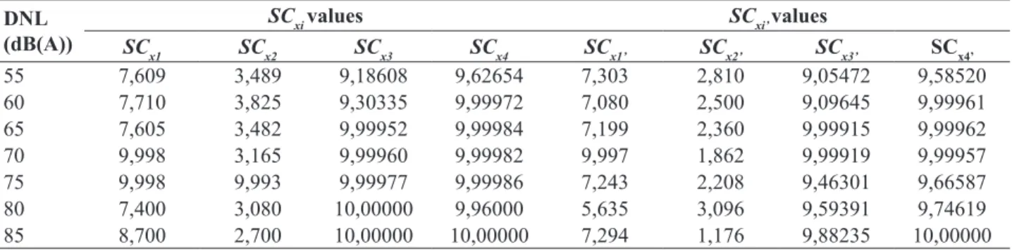
dnL (dB(A))
SC
xi values SCxi’ values
SC
x1 SCx2 SCx3 SCx4 SCx1’ SCx2’ SCx3’ Scx4’
55 7,609 3,489 9,18608 9,62654 7,303 2,810 9,05472 9,58520
60 7,710 3,825 9,30335 9,99972 7,080 2,500 9,09645 9,99961
65 7,605 3,482 9,99952 9,99984 7,199 2,360 9,99915 9,99962
70 9,998 3,165 9,99960 9,99982 9,997 1,862 9,99919 9,99957
75 9,998 9,993 9,99977 9,99986 7,243 2,208 9,46301 9,66587
80 7,400 3,080 10,00000 9,96000 5,635 3,096 9,59391 9,74619
85 8,700 2,700 10,00000 10,00000 7,294 1,176 9,88235 10,00000
Table 4. Values of sensitivity coeficients for different noise curves before and after the aircrafts were removed.
movements. Table 2 presents the values of areas of noise
curves calculated for the respective groups of aircrafts. Calculation was conducted with DNL, as recommended
by RBAC 161 (2011), for different noise curves, and the object of analysis was Guararapes International Airport –
Recife/PE, Brazil (SBRF).
Table 3 presents the values of areas of noise curves calculated after 10% of the aircrafts had been removed
for all movements. Simulations were conducted with the same metrics, resulting in DNL 55, 60, 65, 70, 75, 80 and 85 dB(A) noise curves, with their respective characteristics.
Table 4 presents the sensitivity coeficient values before
(Scxi) and after (cSxi’) 10% of the aircrafts were removed.
Sensitivity variations are more noticeable for bigger
changes in noise curve areas, which were calculated and
are demonstrated in Tables 2 and 3.
From the analysis conducted after obtaining the sensitivity coeficients, it is possible to imply there will be a higher variation in the noise curve areas for the movement variables x3, x4 (Table 2) and x3’, x4’ (Table 3).
The higher the variation of the area of noise curves, the
bigger the reduction of the noise, since the area of the
noise curve will decrease. For movements x1, x2, x1’, x2’,
especially x2, x2’, lower values of sensitivity coeficients
cOncLuSIOnS
Using the sensitivity analysis by computational numerical simulation enables to identify the variations in the most signiicant areas of noise curves that should be carefully analyzed by airport authorities. Since the subject of
airport noise is really relevant in the international context and due to the expectations as to the growth of the aerial
modal, the study of sensitivity analysis can be seen as a tool to help noise control, especially since it enables
identifying which areas of noise curve vary the most. Thus, its use makes measurements to control airport noise more effective.
AcKnOWLEdGEMEnTS
To Instituto alberto Luiz coimbra, of post-graduation and
Research in Engineering of Universidade Federal do Rio
de Janeiro and tothe study group in Airport Noise, which
allowed the performance of this study.
rEFErEncES
ANAC, 2011, “Agência Nacional de Aviação Civil,
Horário de Transportes”, from: http://www.anac.gov.br/
hotran.
Bistalfa, S. R., 2006, “Acústica aplicada ao controle de ruído”, Ed. Edgard Blücher, São Paulo, Brasil.
Federal Aviation Administration, 2009, “Integrated Noise Model, User’s Guide, Versão 7.0”, FAA, Washington, USA.
Code of Federal Regulations 14 CFR 150, 2004, “Noise
Compatibility Planning”, Federal Government of the
United States, Washington, USA.
Gerges, S. N. Y., 2000, “Ruído – Fundamentos e Controles”, 2ª edição, Universidade Federal de Santa Catarina, Florianópolis, Brasil.
Infraero, 2010, “Empresa Brasileira de Infra-Estrutura
Aeroportuária”. from: http://www.infraero.gov.br/index. php/br/navegacao-aerea.html.
International Civil Aviation Organization, 2004, “Final draft of Guidance on the Balanced Approach to Aircraft Noise Management”, Montreal, Canada.
Morais, L. R., Slama, J. G., Mansur, W. J., 2008, “Utilização
de barreiras acústicas no controle de ruído aeroportuário”,
Universidade Federal do Rio de Janeiro, COPPE/PEM /LAVI/ GERA. VII SITRAER, Rio de Janeiro, Brasil. pp. 732-744.