www.atmos-chem-phys.net/15/11981/2015/ doi:10.5194/acp-15-11981-2015
© Author(s) 2015. CC Attribution 3.0 License.
The impact of embedded valleys on daytime pollution transport over
a mountain range
M. N. Lang1, A. Gohm2, and J. S. Wagner3
1Zentralanstalt für Meteorologie und Geodynamik, Vienna, Austria
2Institute of Atmospheric and Cryospheric Sciences, University of Innsbruck, Innsbruck, Austria 3Deutsches Zentrum für Luft- und Raumfahrt, Oberpfaffenhofen, Germany
Correspondence to:M. N. Lang ([email protected])
Received: 16 February 2015 – Published in Atmos. Chem. Phys. Discuss.: 21 May 2015 Revised: 30 September 2015 – Accepted: 16 October 2015 – Published: 28 October 2015
Abstract. Idealized large-eddy simulations were performed to investigate the impact of different mountain geometries on daytime pollution transport by thermally driven winds. The main objective was to determine interactions between plain-to-mountain and slope wind systems, and their influ-ence on the pollution distribution over complex terrain. For this purpose, tracer analyses were conducted over a quasi-two-dimensional mountain range with embedded valleys bor-dered by ridges with different crest heights and a flat foreland in cross-mountain direction. The valley depth was varied sys-tematically. It was found that different flow regimes develop dependent on the valley floor height. In the case of elevated valley floors, the plain-to-mountain wind descends into the potentially warmer valley and replaces the opposing upslope wind. This superimposed plain-to-mountain wind increases the pollution transport towards the main ridge by an addi-tional 20 % compared to the regime with a deep valley. Due to mountain and advective venting, the vertical exchange is 3.6 times higher over complex terrain than over a flat plain. However, the calculated vertical exchange is strongly sensi-tive to the definition of the convecsensi-tive boundary layer height. In summary, the impact of the terrain geometry on the mech-anisms of pollution transport confirms the necessity to ac-count for topographic effects in future boundary layer pa-rameterization schemes.
1 Introduction
Daytime transport and mixing processes of air pollutants pri-marily occur within the convective boundary layer (CBL) and are mostly well understood for flat and homogeneous ter-rain (Steyn et al., 2013). The typical CBL, which forms under fair weather conditions over horizontally homogeneous and flat terrain, consists of a superadiabatic surface layer, a mixed layer (ML), and a stably stratified layer called the entrain-ment layer (EL); the latter separates the CBL from the free at-mosphere (Stull, 1988). Turbulent mixing in the ML induced by rising thermals leads to nearly height-constant profiles of conserved quantities, such as potential temperature and spe-cific humidity up to the EL (Schmidli, 2013; Wagner et al., 2014a). Inside the EL, overshooting thermals cause mixing of potentially cooler air from the ML with air from the sta-bly stratified free atmosphere aloft. This relatively weak ex-change with the free atmosphere limits the vertical dispersion of pollutants mostly to the ML. Over complex terrain, in-teractions between the terrain and the overlying atmosphere lead to a horizontally inhomogeneous CBL structure (Zardi and Whiteman, 2013). Additionally, thermally driven flows increase the vertical transport of pollutants, moisture, and other components. Often this transport goes beyond the CBL top into the free atmosphere (e.g., Gohm et al., 2009; Rotach et al., 2014; Wagner et al., 2014b; Weigel et al., 2007).
as slope winds within the slope layer, valley winds within the valley atmosphere, and plain-to-mountain winds within the mountain atmosphere (Ekhart, 1948; Whiteman, 2000). Under weak synoptic forcing, the interaction of these three wind systems dominates the flow pattern over complex ter-rain (Zardi and Whiteman, 2013).
Observational and modeling studies have shown that ther-mally driven winds and especially upslope winds can en-hance the daytime vertical moisture and mass exchange be-tween the CBL and the free atmosphere over a valley by a factor of 3 to 4 compared to pure turbulent exchange processes over a plain (Henne et al., 2004; Weigel et al., 2007). By means of idealized simulations, Wagner et al. (2014b) show that this increase in vertical transport to the free atmosphere can even be up to 8 times larger depend-ing on the CBL height definition used as the reference sur-face for the vertical transport. In addition to slope and valley winds, vertical transport can be further enhanced by plain-to-mountain winds, which have been explored in the Ver-tical Transport and Orography (VERTIKATOR) campaign (Weissmann et al., 2005) and in several modeling studies (e.g., De Wekker et al., 1998). Plain-to-mountain winds de-velop due to a horizontal temperature gradient between the mountain ridge and the adjacent plain. This mesoscale flow transports low-level air from the foreland to the mountain ridge. The slope winds superposed by the plain-to-mountain winds transport the air further upslope and form vertical up-drafts above the mountain peaks. Under ideal conditions an upper-branch return flow closes the circulation by blowing air from regions above the peaks backwards in the direction of the foreland (De Wekker et al., 1998). This transport pro-cess is referred to as mountain venting and can be an impor-tant additional exchange mechanism between the CBL and the free atmosphere over complex topography (Henne et al., 2004). In more detail, Kossmann et al. (1999) differentiate between mountain venting and advective venting. Both are mesoscale flows exporting CBL air to the free atmosphere, where mountain venting is characterized by a vertical trans-port and advective venting by a horizontal transtrans-port through the CBL top. Advective venting usually occurs if an inclined CBL height exists and the mean wind direction is not parallel to the CBL top (Kossmann et al., 1999).
Thermally driven flows not only provide a vertical trans-port mechanism; they also impact the temperature and hu-midity distribution via horizontal and vertical advection and hence the CBL height over complex terrain. When determin-ing the CBL height based on temperature profiles it is as-sumed that the temperature structure is dominated by vertical mixing. This may often not be the case over complex terrain. Several studies reported shallow (e.g., Adler and Kalthoff, 2014; Rampanelli et al., 2004) or non-existent (e.g., Khoda-yar et al., 2008) mixed layers in valleys, although convec-tion was present. Thus, the definiconvec-tion of the CBL height over complex terrain may be often problematic (e.g., Catalano and Moeng, 2010; Weigel and Rotach, 2004), and many
con-ventional concepts for the determination of the CBL height might not hold for complex topography. Accordingly, the ob-servational and modeling study of De Wekker et al. (2004) shows that during the day, aerosol layer (AL) heights tected with an airborne lidar differ from CBL heights de-termined by temperature-based methods over complex rain, whereas this is not the case over homogeneous, flat ter-rain. Temperature-based CBL heights mostly show a more terrain-following behavior and are lower than AL heights (De Wekker et al., 2004).
As about 50 % of the earth’s land surface consists of moun-tainous terrain (Rotach et al., 2014), differences in trans-port and mixing processes over complex terrain and the flat plain are of great importance for regional weather and cli-mate studies. Today’s operational global numerical weather prediction and climate models have horizontal grid resolu-tions larger than 10 km, which is too coarse to properly re-solve topographically induced transport processes. Present-day boundary layer parameterization schemes are not capa-ble of accounting for these missing subgrid-scale effects (Ro-tach et al., 2014). It is therefore necessary to quantify these effects, e.g., with high-resolution numerical simulations and, based on these results, develop new boundary layer schemes for complex terrain. The need for such a development has already been stressed by Noppel and Fiedler (2002).
This paper relates to recent idealized studies (Wagner et al., 2014b, 2015), which investigate the impact of different valley topographies on the CBL structure, and the vertical exchange between the CBL and the free atmosphere under idealized daytime conditions with a constant surface sensible heat flux. The present work aims at investigating interactions between plain-to-mountain and slope wind systems, and their influence on daytime pollution transport and distribution over complex terrain. This is achieved by tracer analyses over a quasi-two-dimensional mountain range with embedded val-leys and a flat foreland on each side of the mountain in cross-mountain direction. The embedded valleys used in the present simulations are bordered by two mountain ridges of different crest heights. This is in line with a case study of transport processes in a valley with similar asymmetric crest heights (Adler and Kalthoff, 2014) and extends recent ideal-ized simulations of Wagner et al. (2014a, b, 2015) to account for a typical geometric feature of real terrain. Simulations for valleys with different depths are performed and compared to a single-ridge topography to quantify the impact of varying valley floor heights on different transport processes of pollu-tants over complex terrain, e.g., mountain venting and return flows in the free atmosphere.
2 Model and setup
In this study, idealized large-eddy simulations (LES) of day-time thermally driven flows are performed with the Ad-vanced Research version of the Weather Research and Fore-casting model (WRF-ARW), version 3.4. The WRF model is a fully compressible, non-hydrostatic, terrain-following nu-merical modeling system, which can be run in LES mode (Skamarock et al., 2008).
A third-order Runge–Kutta (RK3) time integration scheme, a fifth-order horizontal and a third-order vertical advection scheme are applied in the numerical simulations (Skamarock et al., 2008). Subgrid-scale turbulence is param-eterized by a three-dimensional, 1.5-order turbulent kinetic energy (TKE) closure (Deardorff, 1980). The fully turbu-lent flow is decomposed into its resolved turbuturbu-lent and mean advective parts according to the method of Wagner et al. (2014a), which is described in Sect. 3. A statistics module for online averaging and flux computation has been imple-mented in the WRF model which reduces the demand for data storage.
At the surface a Monin–Obukhov similarity scheme (Monin and Obukhov, 1954) is used to compute turbulent momentum fluxes. This scheme couples the surface and the first model level using the four stability regimes of Zhang and Anthes (1982). The surface roughness length is set to 0.16 m. Following the approach of Wagner et al. (2014a), sur-face moisture fluxes are disabled, and a constant sensible heat flux of 150 W m−2 is prescribed at the surface. These quite substantial simplifications are supported by sensitivity tests performed by Schmidli (2013), which reveal similar flow and CBL developments over an idealized valley when prescrib-ing either a constant or a time-dependent surface sensible heat flux. Further, the recent study of Leukauf et al. (2015) shows an approximately linear relation between the ampli-tude of the sensible heat flux and the ampliampli-tude of the net shortwave radiation. Hence, prescribing the heat flux instead of the radiative forcing will not fundamentally change the re-sults. The simulations are run for 6 h. The resulting integrated heat input would be the same as prescribing a more realis-tic sinusoidal heating with an amplitude of about 235 W m−2 that is reached after 6 h, i.e., at noon. Such heating condi-tions are typical for non-arid mid-latitude valleys (Bonan, 2008; Rotach et al., 2008; Schmidli, 2013). The simulations are initialized with an atmosphere at rest, with a potential temperature of 280 K at sea level height, and a constant ver-tical temperature gradient of 3 K km−1. To avoid moist pro-cesses, the relative humidity is set to a constant value of 40 % at the beginning. To trigger convection, randomly distributed temperature perturbations with amplitudes≤0.5 K are added to the lowermost five model levels. The Rossby number for our problem is about one or larger1suggesting that Coriolis
1Ro=U/(Lf )∼1, with typical values ofU=3 m s−1,L=
30 km, andf=10−4s−1.
force might play some minor role. Nevertheless, for the sake of simplicity we neglect Coriolis effects.
All simulations are performed with a horizontal mesh size of 100 m and 74 vertically stretched levels with a vertical grid spacing increasing from 10 m at the lowest level to 100 m higher aloft. The model top is defined at 6.2 km with a Rayleigh damping layer covering the uppermost 2 km. Pe-riodic lateral boundary conditions are applied in both hori-zontal directions. The integrating time step is set to 0.5 s.
The analytical expression for the quasi-two-dimensional model terrainh(x)is defined as the product of a large-scale mountain h∗(x)with a half width Lx/2 and a small-scale cosine-squared perturbation withn number of wave cycles per length scaleLx:
h(x)=hmaxcos2
x
Lx n π
h∗(x), (1a)
where
h∗(x)=
(
cos2x Lx π
|x| ≤X0
0 |x|> X0
, (1b)
and wherehmaxspecifies the maximum height of the
moun-tain range. This setup is similar to mounmoun-tain configurations with several ridges used in previous studies (Klemp et al., 2003; Schär et al., 2002). In this study, the parameters are set toLx=60 km,X0=30 km, andn=0 or 4. This generates
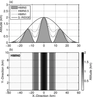
a symmetric, 60 km broad mountain range consisting of a sin-gle ridge forn=0, or three ridges with two embedded val-leys forn=4 (Fig. 1a). In the simulations with three ridges, the ridge atx= −13.9 km and the ridge atx=0 km are here-after referred to as the first and the main ridge, respectively. The slopes are correspondingly counted from left to right: slope 1 (−22.5 km≤x≤ −13.9 km), slope 2 (−13.9 km≤ x≤ −7.5 km), and slope 3 (−7.5 km≤x≤0 km). A flat foreland extends over 30 km on each side of the mountain in cross-mountain direction (see Fig. 1b). The scale of the em-bedded valleys is comparable to real valleys such as the Inn Valley in the European Alps. For sensitivity runs, mountain shapes with elevated valley floors are used, where the topog-raphy is an extension of Eq. (2) and is specified by a linear combination of an upper and lower envelope:
h(x)=(hmax−hmin)cos2 x
Lx n π
h∗(x)+hmin h∗(x), (2)
where h∗(x) is the large-scale mountain of Eq. (2), and wherehmaxandhminare the maximum heights of the upper
and lower envelope, respectively. Whenhminbecomes zero,
Eq. (2) is identical to Eq. (2). In addition to these moun-tain shapes, a simulation over a flat plain is performed. An overview of the different model topographies with their max-imum slope inclinations is given in Table 1.
−30 −20 −10 0 10 20 30 0
0.5 1 1.5 2 2.5 3
Altitude (km)
(a)
HMIN0 HMIN0.5 HMIN1 S−RIDGE
X−Direction (km)
Y−Direction (km)
HMIN0
(b)
−600 −40 −20 0 20 40 60
2 4 6 8 10
Altitude (km)
0.5 1 1.5 2
Figure 1.Idealized model topography of the reference run HMIN0
as(a)vertical cross section (gray shading) and(b)plan view
(show-ing the full domain). Additional topography setups with three ridges and different elevated valley floor heights, and with a single ridge
are used in sensitivity simulations and are shown in(a)as dashed,
dotted and solid lines (compare Table 1).
Table 1.Overview and abbreviations of model topographies as
de-scribed by Eqs. (1) and (2). HMIN0 corresponds to the reference run. All mountain topographies consist of a 60 km broad symmet-ric mountain range with a 30 km wide flat foreland on each side
(see Fig. 1).hmaxandhminare the maximum heights of the upper
and lower envelope, respectively.hvis the effective height of the
valley floor and max(α) the maximum slope inclination. The cases
S-RIDGE and PLAIN refer to sensitivity runs with a single ridge and a flat plain, respectively.
Shape hmax(km) hmin(km) hv(km) max(α) (◦)
PLAIN – – – 0
HMIN0 2 0 0 23
HMIN0.5 2 0.5 0.43 18
HMIN1 2 1 0.84 13
S-RIDGE 2 – – 6
and valleys of constant height inydirection; hence, no valley winds develop in this setup. The computational domain has an extent of 10 km in the along-ridge direction and 120 km in the cross-mountain direction. The idealized terrain in this study is a step towards a more realistic setup compared to recently used idealized topographies consisting of a single valley between two ridges of identical height (e.g. Schmidli,
2012, 2013; Serafin and Zardi, 2010; Wagner et al., 2014a, b, 2015).
Tracer analyses are performed to quantify the impact of different terrain geometries on daytime pollution transport and distribution over a mountain range compared to flat ter-rain. In all simulations, a passive tracer is constantly emitted over the wholey direction within different cross-mountain subdomains, depending on the focus of the analysis. In the vertical, the tracer source covers the lowermost eight model levels (up to an altitude of approximately 110 m), which is comparable to pollution layer depths typically observed in the morning in the Inn Valley (e.g., Gohm et al., 2009). The emission has an arbitrary magnitude. The tracer particles are transported by three-dimensional winds and dispersed by at-mospheric turbulence and diffusion.
3 LES averaging method
In order to distinguish between different heating processes, the flow is decomposed into its mean advective, resolved turbulent, and subgrid-scale parts following the approach of Schmidli (2013) and Wagner et al. (2014a). The fully turbu-lent variableψ (e x, t )is divided into a model grid-box average
ψ (x, t )and a subgrid-scale partψ′(x, t ):
e
ψ (x, t )=ψ (x, t )+ψ′(x, t ). (3)
By means of Reynolds averaging, the model output ψ (x, t )can be formally separated into a mean and a
fluc-tuating part. Therefore, the resolved turbulent partψ′′(x, t )
can be computed from the grid-box average by
ψ′′(x, t )=ψ (x, t )− hψ (x, t )i, (4)
where the time and along-mountain averaging operatorhiis defined as
hi = 1 T Ly
t+ZT /2
t−T /2 Ly
Z
0
ψ (x, t )dydt, (5)
with an averaging interval in time ofT =40 min and in space parallel to mountain range ofLy=10 km. Time averaging is based on a sample interval of 1 min. In order to better com-pare the mean cross-mountain structure of the different sen-sitivity runs, all variables shown in this study are averaged in time and space (alongydirection) according to Eq. (5).
4 CBL height detection
In this study, we distinguish between AL and CBL heights, marking the top of the tracer distribution and the top of the nearly height-constant potential temperature profile, respec-tively. Conventionally, both definitions are synonymously used for the CBL height detection over homogenous and flat terrain. Observational and numerical studies indicate, how-ever, that the heights of the AL and CBL are different over mountainous terrain (De Wekker et al., 2004).
In the present work, the AL height is determined by a gra-dient method computing the vertical gragra-dient extremum2 of aerosol concentration moving upwards from the surface (Emeis et al., 2007). We use three different methods to compute the CBL height. The first one (CBL1) is deter-mined as the height at which the potential temperature gra-dient exceeds a threshold of 0.001 K m−1. This gradient
method is also used by Schmidli (2013) and Wagner et al. (2014b, 2015), whereby the threshold value is chosen fol-lowing Catalano and Moeng (2010). To compare our re-sults with De Wekker et al. (2004), we compute a second CBL height (CBL2) by using the same Richardson-number-based method following Vogelezang and Holtslag (1996). For this purpose, a modified bulk Richardson number is cal-culated on every vertical model level starting from the sur-face. The CBL2 height is then derived as the height where the Richardson number reaches a critical value of 0.25 (Seib-ert et al., 2000; Vogelezang and Holtslag, 1996). A more de-tailed description is given in De Wekker (2002). Seibert et al. (2000) criticize that the Richardson-method of Vogelezang and Holtslag (1996) adds a surface excess temperature to an already existing superadiabatic layer above the ground; therefore, they conclude that the calculated CBL2 height might be slightly overestimated. For comparison, an addi-tional CBL height (CBL3) is calculated based on a Richard-son number method without an additional excess tempera-ture (Seibert et al., 2000). The temporal evolution of hori-zontally averaged AL and CBL heights, vertical sensible heat flux profiles, and normalized tracer mixing ratios over the PLAIN are shown in Fig. 2. Due to the definition of the CBL1 height, it marks the top of the ML and is located slightly be-low the altitude of the vertical heat flux minimum. This is also in line with CBL heights obtained by Schmidli (2013) and Wagner et al. (2014b, 2015). The CBL2 height follows the top of the EL and therefore lies above the CBL1 height (see Fig. 2). During the whole simulation, the vertical posi-tion of the CBL3 is situated in the middle of the EL and is about the same as the AL height in the PLAIN simulation with a homogeneous tracer source near the surface between −30 km≤x≤0 km (see Sect. 2).
For quantifying the vertical transport from the CBL to the free atmosphere, the time dependent CBL1 height is used as
2Technically, the term gradient extremum specifies the
mini-mum value of the negative vertical aerosol gradient.
0.2
0.2
0.4
0.4
0.6
0.6
0.8
0.8
1 1
Time (h)
Altitude (km)
PLAIN−ABL heights
2 3 4 5 6
0 500 1000 1500 2000 2500 3000
Ver
tical Sen
sible
Heatflux (W m
−
2 )
−30
0 30 60 90 120 150 CBL1: grad(Θ) > 0.001 K m−1
CBL2: RI(vog) > 0.25 CBL3: RI(seib) > 0.25 AL: maxgrad(tracer)
Figure 2.Temporal evolution of mean boundary layer heights of
the PLAIN simulation. Shown are three different temperature-based CBL heights and the AL height (see Sect. 4). Thin green contour lines display horizontally averaged normalized tracer mixing ratios (0.1 increment) for a horizontally homogeneous tracer source at the surface. Color contours represent total vertical sensible heat flux profiles of the PLAIN simulation. Due to technical reasons (time
averaging), values are only shown for simulation times after 1.5 h.
reference height. Vertical transport of CBL air beyond this reference height can occur either by turbulent exchange in the EL or by thermally induced circulations.
5 Simulation results 5.1 Flow structure
In this section, the sensitivity of the flow structure on the terrain geometry is assessed. In all simulations the instan-taneous flow is fully turbulent after 2 h of simulation (not shown), and the flow pattern shows similar characteristics to the results in Wagner et al. (2014a). Over the flat foreland a CBL layer and a plain-to-mountain wind is established. In-side the valleys, thermally driven upslope winds develop at the beginning of the simulations.
How-3m s−1
30 25 20 15 10 5 0
X-Direction (km) 0.0 0.5 1.0 1.5 2.0 2.5 3.0 Al ti tu d e (km) HMIN0 (a) 285 286 286 287 288 289 Time = 6 h
-4.0 -3.0 -2.0 -1.0 0.0 1.0 2.0 3.0 4.0 < u > (m s − 1)
3m s−1
30 25 20 15 10 5 0
X-Direction (km) 0.0 0.5 1.0 1.5 2.0 2.5 3.0 Al ti tu d e (km) HMIN0 (e) 285 286 286 287 288 289 Time = 6 h
-1.2 -1.0 -0.8 -0.5 -0.2 0.0 0.2 0.5 0.8 1.0 1.2 < w > (m s − 1)
3m s−1
30 25 20 15 10 5 0
X-Direction (km) 0.0 0.5 1.0 1.5 2.0 2.5 3.0 Al ti tu d e (km) HMIN0.5 (b) 285 286 286 287 288 289 Time = 6 h
-4.0 -3.0 -2.0 -1.0 0.0 1.0 2.0 3.0 4.0 < u > (m s − 1)
3m s−1
30 25 20 15 10 5 0
X-Direction (km) 0.0 0.5 1.0 1.5 2.0 2.5 3.0 Al ti tu d e (km) HMIN0.5 (f) 285 286 286 287 288 289
Time = 6 h
-1.2 -1.0 -0.8 -0.5 -0.2 0.0 0.2 0.5 0.8 1.0 1.2 < w > (m s − 1)
3m s−1
30 25 20 15 10 5 0
X-Direction (km) 0.0 0.5 1.0 1.5 2.0 2.5 3.0 Al ti tu d e (km) HMIN1 (c) 285 286 287 288 289
Time = 6 h
-4.0 -3.0 -2.0 -1.0 0.0 1.0 2.0 3.0 4.0 < u > (m s − 1)
3m s−1
30 25 20 15 10 5 0
X-Direction (km) 0.0 0.5 1.0 1.5 2.0 2.5 3.0 Al ti tu d e (km) HMIN1 (g) 285 286 287 288 289
Time = 6 h
-1.2 -1.0 -0.8 -0.5 -0.2 0.0 0.2 0.5 0.8 1.0 1.2 < w > (m s − 1)
3m s−1
30 25 20 15 10 5 0
X-Direction (km) 0.0 0.5 1.0 1.5 2.0 2.5 3.0 Al ti tu d e (km) S-RIDGE (d) 285 286 287 288 289
Time = 6 h
-4.0 -3.0 -2.0 -1.0 0.0 1.0 2.0 3.0 4.0 < u > (m s − 1)
3m s−1
30 25 20 15 10 5 0
X-Direction (km) 0.0 0.5 1.0 1.5 2.0 2.5 3.0 Al ti tu d e (km) S-RIDGE (h) 285 286 287 288 289
Time = 6 h
-1.2 -1.0 -0.8 -0.5 -0.2 0.0 0.2 0.5 0.8 1.0 1.2 < w > (m s − 1)
Figure 3.Cross sections of averaged(a–d)cross-mountain wind speed and(e–h)vertical wind speed as color contours after 6 h of simulation
for four different mountain shapes: (from top to bottom) HMIN0, HMIN0.5, HMIN1, and S-RIDGE (cf. Table 1). Potential temperature as
black contour lines (0.25 K increment) and wind vectors for components parallel to the cross section. Variables are averaged in time and
<U> (m s−1 ) A lt it u d e ( km)
−4 −2 0 2 4
0 0.5 1 1.5 2 2.5 3 3.5 4
HMIN0, 2 h HMIN0.5, 2 h HMIN0, 4 h HMIN0.5, 4 h (a)
−4 −2 0 2 4
<U> (m s−1 )
A lt it u d e ( km)
−4 −2 0 2 4
0 0.5 1 1.5 2 2.5 3 3.5 4
HMIN0, 2 h HMIN0.5, 2 h HMIN0, 4 h HMIN0.5, 4 h (b)
−4 −2 0 2 4
<U> (m s−1 )
A lt it u d e ( km)
−4 −2 0 2 4
0 0.5 1 1.5 2 2.5 3 3.5 4
HMIN0, 2 h HMIN0.5, 2 h HMIN0, 4 h HMIN0.5, 4 h (c)
−4 −2 0 2 4
Figure 4.Vertical profiles of temporally and spatially averaged cross-mountain wind speed at(a)the middle of slope 1 (x= −18.2 km),
(b) the middle of slope 2 (x= −10.7 km), and the middle of slope 3 (x= −3.7 km) for the mountain shapes HMIN0 (solid lines) and
HMIN0.5 (dashed lines). Black and blue lines are valid for 2 and 4 h of simulation, respectively. Red lines in the inset show the location of the profiles. The averaging in time and space is done according to Eq. (5).
3m s−1
25 20 15 10 5
X-Direction (km) 0.0 0.5 1.0 1.5 2.0 Al ti tu d e (km) HMIN0.5
(a) Time = 2 h
282.0 283.0 284.0 285.0 286.0 < P T > (K )
3m s−1
25 20 15 10 5
X-Direction (km) 0.0 0.5 1.0 1.5 2.0 Al ti tu d e (km) HMIN0.5
(b) Time = 4 h
282.0 283.0 284.0 285.0 286.0 < P T > (K )
3m s−1
25 20 15 10 5
X-Direction (km) 0.0 0.5 1.0 1.5 2.0 Al ti tu d e (km) HMIN0
(c) Time = 4 h
282.0 283.0 284.0 285.0 286.0 < P T > (K )
Figure 5.Cross sections of averaged potential temperature as contour lines (increments of 0.25 K) after(a)2 h and(b)4 h of simulation for
the HMIN0.5 mountain shape and(c)after 4 h for the reference run (HMIN0). Wind vectors for components parallel to the cross section.
Variables are averaged in time and space (alongydirection).
ever, in the reference run (HMIN0, Fig. 3a), due to updrafts in the upper part of slope 2 (cf. naming convention in Sect. 2), the CBL1 height is up to 600 m higher over slope 2 and nearly horizontal over the valley region. In the single-ridge simulation (S-RIDGE, Fig. 3d), the CBL1 height is compa-rable to the one in the simulations with elevated valleys, but the depth3of the CBL is considerably smaller.
Depending on the valley floor height, two different flow regimes develop in the simulations with embedded valleys. The first one occurs in the reference run with the deepest val-ley and the second one in the two simulations with elevated valley floors. In the reference run (HMIN0, Fig. 3a), upslope winds develop over all mountain slopes with cross-mountain wind speeds of up to 2.1 m s−1after 6 h of simulation. In the
3The CBL depth is defined as the CBL height minus the terrain
height.
upper part of slope 2 and above the main ridge updrafts form due to converging upslope winds blowing from both sides of the mountain (Fig. 3e). The convergence zones lead to mean vertical wind speeds of up to 1.3 m s−1and horizontal return flows towards the foreland above the CBL1 height. Above the valley region, subsidence exists with vertical wind speeds of approximately−0.3 m s−1. Over the foreland of the ref-erence run, a plain-to-mountain circulation develops, which surmounts the first ridge and converges over slope 2 with the upslope winds.
<Θ> (K)
A
lt
it
u
d
e
(
km)
Time = 2 h
2820 284 286 288 290 292
0.5 1 1.5 2 2.5 3 3.5 4
HMIN0 HMIN0.5 HMIN1 (a)
282 284 286 288 290 292
<Θ> (K)
A
lt
it
u
d
e
(
km)
Time = 6 h
2820 284 286 288 290 292
0.5 1 1.5 2 2.5 3 3.5 4
HMIN0 HMIN0.5 HMIN1 (b)
282 284 286 288 290 292
Figure 6.Mean vertical profiles of potential temperature after(a)2 h and(b)6 h of simulation for the mountain shapes HMIN0 (solid line),
HMIN0.5 (dashed line), and HMIN1 (dotted line). The vertical profiles are vertically interpolated from model levels to constant height levels
and horizontally averaged between the first and main ridge (−13.9 km≤x≤0 km, see red area in insets). Variables are averaged in time and
space (alongydirection) according to Eq. (5).
HMIN0
Heating rate (10
−3
K s
−1
)
Time (h) (a)
2 3 4 5 6
−0.2 −0.1 0 0.1 0.2
HMIN1
Heating rate (10
−3
K s
−1
)
Time (h) (b)
2 3 4 5 6
−0.2 −0.1 0 0.1 0.2
TOT SHF ADV TRB
Figure 7.Evolution of density-weighted and volume-averaged heat budget components for(a)the HMIN0 and(b)the HMIN1 simulation.
The total tendency (TOT) is equal to the sum of surface sensible heat flux (SHF), mean flow advection (ADV), and turbulent exchange
(TRB). Both control volumes extend from the first to the main ridge and from the surface to an altitude of 2.1 km. Due to technical reasons
(time averaging), values are only shown after 1.5 h of simulation.
0.5 km compared to the HMIN0 run. Furthermore, the deeper slope wind layer prevents subsidence in the center of the val-ley. Due to the absence of a convergence zone above the first ridge in the HMIN0.5 and HMIN1 simulation, updrafts and return flows only develop over the main ridge. This leads to a single return flow above the CBL1 height towards the foreland with wind speeds up to 2.2 m s−1(between 1.4 and 2.6 km), whereas in the reference run (HMIN0), two nearly separated return flows develop over the foreland with wind speeds less than 1.9 m s−1(between 1.4 and 1.8 km, and be-tween 2.1 and 2.5 km).
In the S-RIDGE simulation, an upslope wind layer su-perposed by the plain-to-mountain wind develops with wind
speeds up to 2.4 m s−1 and a layer depth of approximately 400 m. The return flow towards the foreland is divided into two clearly separated wind layers: an upper one above crest height (between 2.2 and 2.9 km), which is deeper and has stronger winds (up to 1.4 m s−1), and a lower one, which is
located slightly above the CBL1 height with wind speeds be-low 0.6 m s−1.
Normalized Mixing Ratio 0.2 0.4 0.6 0.8 1
X−Direction (km)
−30 −25 −20 −15 −10 −5 0
0 4 8
Altitude (km)
Time = 6 h
PLAIN
(a)
284
285 286 287 288 289
0 0.5 1 1.5 2 2.5 3
Normalized Mixing Ratio
0.2 0.4 0.6 0.8 1
X−Direction (km)
−30 −25 −20 −15 −10 −5 0
0 4 8
Altitude (km)
Time = 6 h
HMIN0
(b)
285
285
286 287 288 289
0 0.5 1 1.5 2 2.5 3
Normalized Mixing Ratio
0.2 0.4 0.6 0.8 1
X−Direction (km)
−30 −25 −20 −15 −10 −5 0
0 4 8
Altitude (km)
Time = 6 h
HMIN0.5
(c)
285
285
286
286 287
288 289
0 0.5 1 1.5 2 2.5 3
Normalized Mixing Ratio
0.2 0.4 0.6 0.8 1
X−Direction (km)
−30 −25 −20 −15 −10 −5 0
0 4 8
Altitude (km)
Time = 6 h
HMIN1
(d)
285
285
286
286
287 288 289
0 0.5 1 1.5 2 2.5 3
Normalized Mixing Ratio
0.2 0.4 0.6 0.8 1
X−Direction (km)
Mass (% km
⁻
¹)
−30 −25 −20 −15 −10 −5 0
0 4 8
Altitude (km)
Time = 6 h
S−RIDGE
(e)
285
285
286
286
287
287
287
288 289
0 0.5 1 1.5 2 2.5 3
CBL1: grad(Θ) > 0.001 K m−1 CBL2: RI(vog) > 0.25 CBL3: RI(seib) > 0.25 AL: maxgrad(tracer)
Mass (% km
⁻
¹)
Mass (% km
⁻
¹)
Mass (% km
⁻
¹)
Mass (% km
⁻
¹)
Figure 8.Cross sections of tracer concentrations (color contours) after 6 h of simulation for all simulations:(a)PLAIN,(b)HMIN0,(c)
HMIN0.5,(d)HMIN1, and(e)S-RIDGE. A passive tracer has been constantly emitted over the whole along-mountain domain within the
region of−30 km≤x≤0 km on the lowermost eight model levels (up to an altitude of approximately 110 m). Mixing ratios are averaged
in time and space (alongydirection), and normalized by their corresponding maximum value. CBL heights CBL1, CBL2, CBL3, and AL
are plotted as black solid, dashed, dotted, and green solid lines, respectively (see also the legend shown in Fig. 8e). Potential temperature is
shown as black contour lines (0.25 K increment). Additionally, vertically integrated tracer masses are shown for 2, 4, and 6 h of simulation
as dotted, dashed, and solid lines in the bottom panels, respectively. These relative mass values are calculated by splitting thexdirection into
bins of 1 km and determining the percentage of total amount of tracers within these cross-mountain intervals (% km−1).
over all slopes. The depth of the slope wind layer is shallower over slope 3 (Fig. 4c) than over slope 1 and 2 (Fig. 4a, b). Prandtl’s (1944) analytical slope-wind model predicts shal-lower slope winds for steeper slopes and higher static
of simulation, the plain-to-mountain flow overruns the first peak, accelerates over slope 2 and finally reaches the ele-vated valley floor. The downslope flow has a speed of about 3.8 m s−1and a depth of approximately 500 m (Fig. 4b). In the reference run, however, the upslope wind regime persists throughout the simulation and hinders the plain-to-mountain wind to penetrate into the valley. The evolution of differ-ent flow regimes was mainly caused by differdiffer-ent temperature structures. This is discussed in detail in Sect. 5.2.
5.2 Temperature structure
In this section, differences in the temperature structure due to varying terrain geometries are described and explained by means of differences in heating rates. To demonstrate the evolution of the downslope wind within the elevated valley, cross sections of potential temperature are displayed for the HMIN0 and HMIN0.5 simulation in Fig. 5. After 2 h in the HMIN0.5 simulation (Fig. 5a), the air over the first ridge, ad-vected by the plain-to-mountain flow from the foreland, is potentially cooler than the valley air and therefore able to de-scend into the valley. Due to a weakening of the upslope wind over slope 2, the convergence zone is continuously shifted towards the valley floor and the downslope flow eventually replaces the local slope wind circulation after 4 h of simu-lation (Fig. 5b). In the reference run after 4 h of simusimu-lation (Fig. 5c), the advected air at crest height over the first ridge has about the same potential temperature than the air in the upslope flow advected from the valley. Due to the deeper val-ley in HMIN0 compared to the elevated valval-leys in HMIN0.5 and HMIN1, a more distinctive upslope circulation estab-lishes over slope 2. Both facts prevent the plain-to-mountain wind to descend to the valley floor during the entire simula-tion.
The convergence zone is characterized by two thermally driven opposing flows that separate from the surface. Flow separation may also occur over steep slopes for dynamical reasons without the need of a strong counter current in the valley. This has been shown in several studies of stably strat-ified flows past a valley based on idealized simulations (e.g., Vosper and Brown, 2008) and laboratory experiments (e.g., Lee et al., 1987; Tampieri and Hunt, 1985). For example, a critical valley depth may exist beyond which the valley at-mosphere becomes decoupled from the imposed background flow aloft (e.g., Vosper and Brown, 2008). However, a more detailed study to clarify the dependence of the depth of flow penetration into the valley as a function of the valley depth would go beyond the scope of this paper.
Mean vertical profiles of potential temperature over the valley region are shown for all simulations with valleys in Fig. 6. After 2 h of simulation (Fig. 6a), potential tempera-tures near the valley floor are approximately 1 to 2 K colder in the reference run (HMIN0) compared to the simulations with elevated valleys (HMIN0.5, HMIN1). The mean poten-tial temperature profile of the reference run shows a
three-layer thermal structure over the valley region with a well-mixed layer (CBL1), a valley inversion layer and an upper weakly stable layer (Vergeiner and Dreiseitl, 1987; Schmidli, 2013). After 6 h of simulation (Fig. 6b), all profiles show nearly identical mean potential temperatures with a well-mixed CBL1 up to approximately 1.8 km.
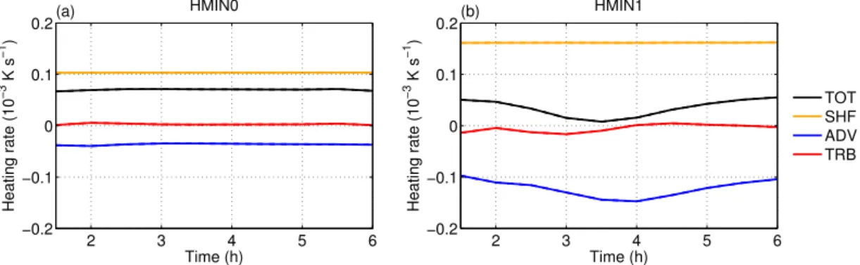
To investigate the reason for these different potential temperature profiles, density-weighted and volume-averaged heating rates are computed for the largest (HMIN0) and the smallest valley volume (HMIN1) according to the method of Schmidli (2013). Both control volumes extend from the first to the main ridge and from the surface to an altitude of 2.1 km. In Fig. 7, the evolution of all heat budget com-ponents is shown, where the total tendency (TOT) is equal to the sum of the contributions due to the surface sensible heat flux (SHF), the mean flow advection (ADV), and the turbulent heat exchange between the valley volume and the free atmosphere (TRB). Due to the flux computation method used in this study, which involves averaging in time, no heat-ing rates could be calculated before 1.5 h of simulation. Nev-ertheless, potential temperature profiles indicate that in the early phase (before 2 h) the heating is stronger for smaller valley volumes than for larger ones (cf. HMIN1 and HMIN0 in Fig. 6a). The result is in agreement with the concept of the valley-volume effect which states that for a given amount of energy input, the heating rate is stronger the smaller the volume (e.g., Wagner, 1932). This explains why the heating rate contribution from the surface sensible heat flux (SHF) is permanently higher in the simulation with smaller valley volume (HMIN1) compared to the reference run with larger valley volume (HMIN0, cf. Fig. 7), although the surface sen-sible heat flux itself is the same in both simulations. Figure 7 shows that the surface sensible heat flux is the main heating source of the valley atmosphere in both simulations, whereas mean-flow advection (ADV) cools the valley volume, and the turbulent contributions (TRB) are negligible. In contrast to the early phase, the total heating rate (TOT) of the HMIN1 simulation is smaller than of the HMIN0 run after about 1.5 h (Fig. 7). The reason is that the plain-to-mountain flow enters the control volume of the HMIN1 run and leads to a much stronger cold-air advection (ADV) than in HMIN0. Conse-quently, advection overcompensates the volume effect. This striking heating pattern leads to the almost same potential temperatures in the CBL until the end of all simulations (see Fig. 6b), despite the different valley volumes.
5.3 Pollution distribution
Simulation time
Relative tracer mass (%)
Tracer source between −30 km ≤ x ≤ 0 km
PLAIN HMIN0 HMIN0.5 HMIN1 S−RIDGE PLAIN HMIN0 HMIN0.5 HMIN1 S−RIDGE PLAIN HMIN0 HMIN0.5 HMIN1 S−RIDGE PLAIN HMIN0 HMIN0.5 HMIN1 S−RIDGE
2 h 3 h 4 h 5 h 6 h 0
20 40 60 80 100
above CBL1 below CBL1
Figure 9.Relative tracer mass located above (dark gray) and below (light gray) the reference CBL height (CBL1) as a function of time.
A tracer has been constantly emitted near the surface over the half space of the mountain range within the region of−30 km≤x≤0 km (see
Fig. 8). Shown are all simulations (from left to right) between 2 and 6 h: PLAIN, HMIN0, HMIN0.5, HMIN1, and S-RIDGE.
Normalized Mixing Ratio
0.2 0.4 0.6 0.8 1
X−Direction (km)
−30 −25 −20 −15 −10 −5 0
0 10 20 30
Altitude (km)
Time = 6 h
HMIN0 (a)
285
285 286
287 288 289
0 0.5 1 1.5 2 2.5
3 CBL1: grad(Θ) > 0.001 K m−1
Normalized Mixing Ratio
0.2 0.4 0.6 0.8 1
X−Direction (km)
Mass (% km
⁻
¹)
−30 −25 −20 −15 −10 −5 0
0 10 20 30
Altitude (km)
Time = 6 h
HMIN0.5 (b)
285
285
286
286
287 288 289
0 0.5 1 1.5 2 2.5
3 CBL1: grad(Θ) > 0.001 K m−1
Normalized Mixing Ratio
0.2 0.4 0.6 0.8 1
X−Direction (km)
Mass (% km
⁻
¹)
−30 −25 −20 −15 −10 −5 0
0 10 20 30
Altitude (km)
Time = 6 h
S−RIDGE
(c)
285
285 286
286
287 287
287 288
289
0 0.5 1 1.5 2 2.5 3
CBL1: grad(Θ) > 0.001 K m−1
Mass (% km
⁻
¹)
Figure 10.As in Fig. 8 for the(a)HMIN0,(b)HMIN0.5, and(c)S-RIDGE simulation, but a tracer has been constantly emitted within the
Normalized Mixing Ratio 0.2 0.4 0.6 0.8 1
X−Direction (km)
Mass (% km
⁻
¹)
−30 −25 −20 −15 −10 −5 0
0 10 20 30
Altitude (km)
Time = 6 h
HMIN0 (a)
285
285
286 287 288 289
0 0.5 1 1.5 2 2.5
3 CBL1: grad(Θ) > 0.001 K m−1
Normalized Mixing Ratio
0.2 0.4 0.6 0.8 1
X−Direction (km)
Mass (% km
⁻
¹)
−30 −25 −20 −15 −10 −5 0
0 10 20 30
Altitude (km)
Time = 6 h
HMIN0.5 (b)
285
285 286
286
287 288 289
0 0.5 1 1.5 2 2.5
3 CBL1: grad(Θ) > 0.001 K m−1
Figure 11.As in Fig. 8 for the(a)HMIN0 and(b)HMIN0.5
sim-ulation, but a tracer has been constantly emitted at the foot of the
mountain range between−23 km≤x≤ −22 km.
section, Sect. 5.4, is on the impact of the valley floor height on processes of pollution transport over complex terrain.
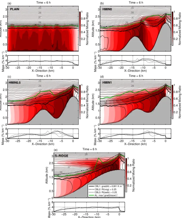
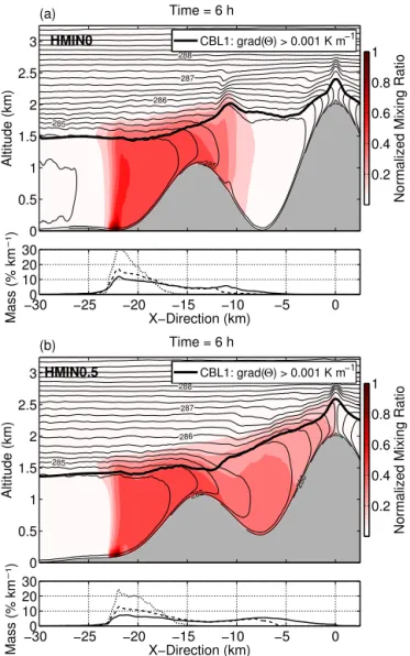
In the first step, a passive tracer is constantly emitted at the surface over the half space of the mountain range within the region of−30 km≤x≤0 km (see Sect. 2). Figure 8 shows cross sections of normalized tracer mixing ratios, and the AL and CBL heights for all simulations after 6 h of inte-gration. The mixing ratio has been normalized by its maxi-mum value occurring in the shown domain at the given time. Additionally, vertically integrated tracer masses are shown for 2, 4, and 6 h of simulation. In the PLAIN simulation (Fig. 8a), the turbulent transport results in a nearly homo-geneous distribution of tracer particles inside the CBL up the EL. The CBL1 height marks the top of the nearly height-constant potential temperatures at 1.7 km. The altitude of the AL height is located at approximately 1.9 km and lies be-tween the heights of the CBL2 and CBL3. The almost
iden-tical CBL and AL heights over the plain qualitatively con-firm results of De Wekker et al. (2004). The vertically in-tegrated tracer mass is homogeneously distributed with ap-proximately 3.3 % km−1. This results in slightly less than 100 % tracer mass when integrating between−30 km≤x≤ 0 km, as a small part of tracer mass is horizontally trans-ported out of this subdomain due to turbulent diffusion. In the reference run (Fig. 8b), tracer particles are advected to-wards both ridges by upslope winds. After 6 h of simula-tion, concentration maxima exist in regions of updrafts over slope 2 (−13 km≤x≤ −11 km) and in the upper part of slope 3 (−1 km≤x≤ −0 km). Therefore, the largest tracer masses are found with up to 5.9 % km−1over the valley re-gion after 6 h of simulation. The AL and CBL heights over the foreland are in all simulations similar to the ones in the plain simulation. Over the valley region of the reference run (−9 km≤x≤ −3 km), the AL height is considerably higher (up to 0.8 km for CBL1) than the CBL heights. In the HMIN0.5 (Fig. 8c) and HMIN1 (Fig. 8d) run, the superim-posed plain-to-mountain flow leads to a less complex tracer distribution than in the HMIN0 case with a rather continuous horizontal increase in tracer mass towards the main ridge. In the regionx <−8 km, the AL heights are considerably higher (up to 0.9 km for CBL1) than the CBL heights. As in the reference run, this implies a tracer transport towards higher altitudes than the temperature-based CBL heights. In the S-RIDGE simulation a second tracer maximum above crest height exists at approximately 2.5 km. The total hori-zontal mass flux of tracer particles in the return flow above the CBL is only sightly higher in the S-RIDGE run than in the other simulations (not shown) and, hence, cannot explain the formation of the elevated layer of tracers in S-RIDGE. However, the center of the return flow is located about 500 m higher in S-RIDGE which favors the formation of a pollution layer at this height compared to the other runs (cf. Figs. 3 and 8). Generally, similar elevated pollution maxima were mod-eled by Fiedler et al. (2002) and elevated moist layers down-stream of mountain ridges related to advective venting were observed by Adler et al. (2015).
These results corroborate the concept of an additional transport between the CBL and the free atmosphere over complex terrain in comparison to a pure convective exchange process (De Wekker et al., 2004). The CBL heights show a more terrain-following behavior than the AL height for all simulations except for the HMIN0 run. In that simulation, the different CBL heights are nearly horizontal over the val-ley region as a result of a strong updraft over slope 2 (cf. Sect. 5.1). Nevertheless, the CBL heights are still lower than the AL height. The comparison of the present results with those of De Wekker et al. (2004), who used the same CBL height definition as our CBL2, shows similar differences be-tween the AL and CBL2 heights (up to 0.4 km) for various terrain geometries.
Simulation time
Relative tracer mass (%)
Tracer source between −23 km ≤ x ≤ −22 km
S−RIDGE HMIN1 HMIN0.5 HMIN0 S−RIDGE HMIN1 HMIN0.5 HMIN0 S−RIDGE HMIN1 HMIN0.5 HMIN0 S−RIDGE HMIN1 HMIN0.5 HMIN0 S−RIDGE HMIN1 HMIN0.5 HMIN0
2 h 3 h 4 h 5 h 6 h
0 20 40 60 80 100
left of smaller ridge right of smaller ridge
Figure 12.Relative tracer mass located left (light gray) and right (dark gray) of the first ridge (x= −13.9 km) as a function of time. A tracer
has been constantly emitted at the foot of the mountain range (−23 km≤x≤ −22 km, see Fig. 11). Shown are the simulations HMIN0,
HMIN0.5, HMIN1, and S-RIDGE between 2 and 6 h of simulation.
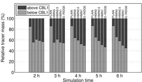
a flat plain, the only process to transport pollutants into the free atmosphere is turbulent mixing in the EL. Therefore, in the PLAIN simulation nearly all of the tracer particles (up to 85 %) stay below the CBL1 height throughout the entire sim-ulation. In contrast to the PLAIN run, approximately 40 % of tracer mass is located above the CBL1 height after 2 h in the simulations with mountains. Until the end of the sim-ulation, the vertical transport beyond the CBL1 height in-creases up to 50 % for the HMIN1 case and up to 55 % for the S-RIDGE simulation. In the reference run, the relative tracer mass above the CBL1 height compared to the relative tracer mass within the CBL slightly decreases to 35 % un-til the simulation end. This decrease in relative tracer mass above the CBL1 height is due to the fact that the constant tracer source at the surface is stronger than the vertical tracer transport through the CBL top. In summary, topographically induced vertical tracer transport from the surface to the free atmosphere can be up to 2.5 to 3.7 times larger than pure tur-bulent exchange over a flat plain. Similar results were found for the vertical transport out of a valley in the real-case study of Weigel et al. (2007) and in the idealized modeling study of Wagner et al. (2014b). Repeating the same analysis of tracer exchange for the CBL3 as a reference height instead of CBL1 leads to the same qualitative results. However, in terms of quantitative exchange, the vertical transport is three times (5.5 to 10.3) higher for CBL3 than for CBL1. This
re-sult demonstrates the strong sensitivity of the magnitude of the vertical exchange on the definition of the CBL height. 5.4 Pollution transport processes
This section focuses on the impact of embedded valleys and varying valley floor heights on different transport mecha-nisms, such as mountain venting in updrafts and advective venting by horizontal return flows. To isolate individual hor-izontal and vertical transport processes, a passive tracer is constantly emitted within three different subdomains: over the slope within the mountain range, at the foot of the moun-tain range, and over the valley floor, respectively.
def-Normalized Mixing Ratio 0.2 0.4 0.6 0.8 1
Altitude (km)
Time = 6 h
HMIN0 (a)
285
285
286
286 287
288 289
Normalized Mixing Ratio
0.2 0.4 0.6 0.8 1
X−Direction (km)
Mass (% km
⁻
¹)
−30 −25 −20 −15 −10 −5 0
0 10 20 30
Altitude (km)
Time = 6 h
HMIN0.5 (b)
285
285 286
286
287 288 289
X−Direction (km)
Mass (% km
⁻
¹)
−30 −25 −20 −15 −10 −5 0
0 10 20 30 0 0.5 1 1.5 2 2.5
3 CBL1: grad(Θ) > 0.001 K m−1
0 0.5 1 1.5 2 2.5
3 CBL1: grad(Θ) > 0.001 K m−1
Figure 13.As in Fig. 8 for the(a)HMIN0 and(b)HMIN0.5
sim-ulation, but a tracer has been constantly emitted at the valley floor
between−8 km≤x≤ −7 km.
inition of Kossmann et al. (1999), mainly mountain venting occurs in these simulations. Closer inspections (not shown) of the flow structure indicate, that in the S-RIDGE simula-tion, both mountain and advective venting occur to the same extent (cf. Figs. 3 and 10c).
As previously noticed, difference in the return flow struc-ture (cf. Fig. 3) cause different patterns of horizontal tracer transport from the main ridge towards the foreland (Fig. 10). In the HMIN0 simulation (Fig. 10a), the additional venting process over slope 2 prevents a horizontal transport of pol-lutants from the main ridge towards the foreland beyond the valley region. Due to the absence of updrafts over the smaller ridge in the HMIN0.5 simulation (Fig. 10b), the tracers are transported by the more homogeneous return flow almost twice the horizontal distance towards the foreland compared to the HMIN0 run. In the S-RIDGE simulation (Fig. 10c), a distinct return flow develops, which extends approximately
500 m higher up to about 3 km than in the other simula-tions. This leads to the previously mentioned elevated tracer layer shown in Fig. 8. These different distribution patterns are also represented in the vertically integrated tracer masses. At the end of the simulation, the integrated tracer mass in the HMIN0.5 and S-RIDGE is more evenly distributed between −20 km≤x≤0 km and −30 km≤x≤0 km, respectively, whereas in the HMIN0 run a non-uniform tracer distribution remains with a mass maximum over the valley region.
To investigate the pollution transport from the foreland to-wards the mountain crest, a passive tracer is emitted at the foot of the mountain range between−23 km≤x≤ −22 km, which is shown for the HMIN0 and HMIN0.5 simulation in Fig. 11. Until the end of the HMIN0 simulation (Fig. 11a), tracer particles are transported horizontally by the plain-to-mountain flow up to the convergence zone in the upper part of slope 2 (x≃ −12 km). From there, particles are transported to higher altitudes within the updraft. Apart from this pro-nounced and stationary updraft, moving thermals distribute the tracers relatively homogeneously in the vertical up to the CBL1 height. In contrast to the reference run, the tracer parti-cles in the HMIN0.5 simulation are transported horizontally up to the main ridge (x=0 km) until the end of the simula-tion (Fig. 11b).
Simulation time
Relative tracer mass (%)
Tracer source between −8 km ≤ x ≤ −7 km
HMIN0 HMIN0.5 HMIN1 HMIN0 HMIN0.5 HMIN1 HMIN0 HMIN0.5 HMIN1 HMIN0 HMIN0.5 HMIN1
2 h 3 h 4 h 5 h 6 h
0 20 40 60 80 100
above CBL1 below CBL1
Figure 14.Relative tracer mass located above (dark gray) and below (light gray) the reference CBL height (CBL1) as a function of time.
A tracer has been constantly emitted at the valley floor (−8 km≤x≤ −7 km, see Fig. 13). Shown are all simulations with valleys (from left
to right) between 2 and 6 h: HMIN0, HMIN0.5, and HMIN1.
To study the pollution transport within a mountain val-ley, a passive tracer is emitted at the valley floor between −8 km≤x≤ −7 km, which is shown in Fig. 13 for the HMIN0 and HMIN0.5 simulation. Due to the existence of the typical slope wind system within the valley in the ref-erence run (Fig. 13a), subsidence above the valley center mainly limits the tracer transport to the valley region and most tracer particles remain below the CBL1 height during the whole simulation. In the HMIN0.5 run (Fig. 13b), tracers are transported by the superimposed plain-to-mountain wind towards the main peak and within the updraft to the free tro-posphere. From there, the tracer is transported by the return flow towards the foreland.
The vertical part of this transport by mountain and advec-tive venting is quantified for all simulations with valleys in Fig. 14. After 2 h, the turbulent transport by convection is the dominant process for the tracer distribution and barely 20 to 25 % of the tracer mass is mixed beyond the CBL1 height. After 3 h in the HMIN1 and 5 h in the HMIN0.5 sim-ulation, the distribution pattern changes due to the additional tracer transport by the plain-to-mountain wind within the val-ley. Therefore, until the end of the simulations with elevated valleys (HMIN0.5, HMIN1), up to 60 % of the tracer parti-cles are advected beyond the CBL1 height. However, in the reference run only 30 % of the emitted tracer mass is located above the CBL1 height due to subsidence in the valley cen-ter and a missing superimposed cross-mountain flow. Com-paring tracer emissions within different cross-mountain sub-domains (e.g., Figs. 10 and 13), reveals that in all simula-tions with valleys mountain and advective venting occurs; but whether pollutants emitted at the valley floor are trans-ported out of the valley depends on the interactions between the plain-to-mountain and the slope wind systems.
6 Conclusions
In this study we performed idealized LES with the WRF model to investigate the interaction between plain-to-mountain and slope wind systems, and their influence on day-time pollution distribution over complex terrain. Simulations over a mountain range with embedded valleys bordered by ridges with different crest heights were compared to simula-tions with a single ridge and a flat plain by means of tracer analyses.
These analyses show differences in thermally driven flows and resultant pollution transport dependent on the valley floor heights. To illustrate the observed two main flow pat-terns, a conceptual diagram is shown in Fig. 15. In the situ-ation of a deep valley (reference run HMIN0, Fig. 15a), the upslope wind system within the valley opposes the plain-to-mountain wind and therefore acts as an effective “barrier” between the foreland and the main ridge. In the situation of a shallow, elevated valley (e.g., HMIN0.5, Fig. 15b), the plain-to-mountain flow passes the crest of the first (smaller) ridge, descends into the potentially warmer valley, and even-tually replaces the opposing upslope wind. These two differ-ing flow structures lead to different transport patterns. In the reference run, less than 30 % of tracer particles emitted over the foreland are advected beyond the first ridge towards the main ridge until the end of the simulation. However, in the simulations with elevated valleys, the relative tracer mass lo-cated on the right-hand side of the first ridge is similar to that of a simulation with a single ridge and amounts to approxi-mately 50 %.
V
B
V
AL
CBL Deep valley (HMIN0)
AL
V
CBL
Elevated valley (HMIN0.5)
Figure 15.Conceptual diagram of the flow pattern for(a)a deep
valley (HMIN0) and(b)an elevated valley (e.g., HMIN0.5) after 6 h
of simulation. The black and gray solid lines mark the temperature-based CBL and the AL height, respectively. Thick, solid arrows represent the cross-mountain flow, and thin, solid arrows mark the turbulent exchange in the entrainment layer over the foreland and the valley region. Dashed, double-lined arrows indicate the vertical transport through the CBL top as a result of horizontal flow
conver-gence.V denotes mountain and advective venting and B indicates
flow blocking.
turbulent exchange by convection. Pollutants are transported within the slope wind layers towards the mountain ridges, and within the vertical updrafts above the CBL height. From there, the pollutants are captured by the horizontal return flow and are advected towards the foreland. The determina-tion whether mountain or advective venting occurs strongly depends on the reference surface through which the trans-port is assessed. It also depends on which part of the updraft is considered (the center or the outflow region). The simula-tions show that independent of this detail, the exchange by venting, be it mountain or advective venting, is caused by the same stationary updraft as a result of horizontal flow con-vergence over the ridges. Therefore, we suggest that at least for purely thermally driven winds without a large-scale flow no distinction between mountain and advective venting is needed, as already done, e.g., in Henne et al. (2004, 2005). In the simulations with elevated valleys, the plain-to-mountain flow covers the whole mountain range and therefore prevents the development of venting over the first ridge.
The detected AL and CBL heights are in line with the re-sults obtained by De Wekker et al. (2004). Over the flat plain, the spread between the temperature-based CBL heights and the AL height is rather small. However, over complex terrain, the CBL heights are up to 0.9 km lower and rather terrain-following than the AL height. In the present simulations, the mountain induced vertical transport beyond the CBL1 height is up to 3.6 times larger than pure turbulent exchange over a flat plain. Even though the quantification of the vertical ex-change strongly depends on the definition of the CBL, the significant transport beyond the CBL1 height in the present simulations demonstrates the need to consider the AL height rather than temperature-based CBL heights as the relevant parameter for air pollution studies over mountainous terrain. The results of this study extend those of Wagner et al. (2014b, 2015), and confirm that the terrain geometry has a large impact on the flow structure and the resultant trans-port processes over a mountain range. The change of the flow regime due to minor changes in the topography demonstrates the necessity to account for these topographically induced effects in future boundary layer parameterization schemes. Furthermore, the findings confirm a mountain-induced ver-tical transport of pollutants beyond the temperature-based CBL height and therefore imply a reconsideration of the con-ventional CBL height detection methods over mountainous terrain. However, to generalize present findings, further in-vestigations with inhomogeneous land-use properties, time and space dependent surface forcings, and varying atmo-spheric background conditions will be necessary.
Acknowledgements. This work was supported by the Austrian Science Fund (FWF) under grant P23918-N21 and by the Austrian Federal Ministry of Science Research and Economy (BMWF) as part of the Uni-Infrastrukturprogramm of the Research Platform Scientific Computing at the University of Innsbruck. We greatly appreciate the comments of two anonymous reviewers, which have considerably improved the paper.
Edited by: W. Birmili
References
Adler, B. and Kalthoff, N.: Multi-scale transport processes ob-served in the boundary layer over a mountainous island, Bound.-Lay. Meteorol., 153, 515–537, doi:10.1007/s10546-014-9957-8, 2014.
Adler, B., Kalthoff, N., Kohler, M., Handwerker, J., Wieser, A., Corsmeier, U., Kottmeier, C., Lambert, D., and Bock, O.: The variability of water vapour and pre-convective conditions over the mountainous island of Corsica, Q. J. Roy. Meteorol. Soc., doi:10.1002/qj.2545, online first, 2015.
Catalano, F. and Moeng, C.: Large-eddy simulation of the daytime boundary layer in an idealized valley using the Weather Research and Forecasting numerical model, Bound.-Lay. Meteorol., 137, 49–75, doi:10.1007/s10546-010-9518-8, 2010.
Deardorff, J. W.: Stratocumulus-capped mixed layers derived from a 3-dimensional model, Bound.-Lay. Meteorol., 18, 495–527, doi:10.1007/BF00119502, 1980.
De Wekker, S. F. J.: Structure and morphology of the convective boundary layer in mountainous terrain, PhD thesis, University of British Columbia, Department of Earth and Ocean Sciences, Vancouver, 2002.
De Wekker, S. F. J., Zhong, S., Fast, J. D., and Whiteman, C. D.: A numerical study of the thermally driven plain-to-basin wind over idealized basin topographies, J. Appl. Meteorol., 37, 606–622, doi:10.1175/1520-0450(1998)037<0606:ANSOTT>2.0.CO;2, 1998.
De Wekker, S. F. J., Steyn, D. G., and Nyeki, S.: A comparison of aerosol-layer and convective boundary-layer structure over a mountain range during Staaarte ’97, Bound.-Lay. Meteorol., 113, 249–271, doi:10.1023/B:BOUN.0000039371.41823.37, 2004. Ekhart, E.: De la structure thermique de l’atmosphere dans la
mon-tagne (On the thermal structure of the mountain atmosphere), La Meteorologie, 4, 3–26, 1948, English translation: White-man, C. D. and Dreiseitl, E., 1984, Alpine meteorology: Trans-lations of classic contributions by: Wagner, A., Ekhart E., and Defant, F., PNL–5141/ASCOT–84–3, Pacific Northwest Labora-tory, Richland, Washington, 121 pp., 1948.
Emeis, S., Jahn, C., Münkel, C., Münsterer, C., and Schäfer, K.: Multiple atmospheric layering and mixing-layer height in the Inn valley observed by remote sensing, Meteorol. Z., 16, 415–424, doi:10.1127/0941-2948/2007/0203, 2007.
Fiedler, F., Bischoff-Gauß, I., Kalthoff, N., Adrian, G.: Mod-eling of the transport and diffusion of a tracer in the Freiburg-Schauinsland area, J. Geophys. Res., 105, 1599–1610, doi:10.1029/1999JD900911, 2000.
Gohm, A., Harnisch, F., Vergeiner, J., Obleitner, F.,
Schnitzhofer, R., Hansel, A., Fix, A., Neininger, B., Emeis, S., and Schäfer, K.: Air pollution transport in an Alpine valley: Results from airborne and ground-based observations, Bound.-Lay. Meteorol., 131, 441–463, doi:10.1007/s10546-009-9371-9, 2009.
Henne, S., Furger, M., Nyeki, S., Steinbacher, M., Neininger, B., de Wekker, S. F. J., Dommen, J., Spichtinger, N., Stohl, A., and Prévôt, A. S. H.: Quantification of topographic venting of bound-ary layer air to the free troposphere, Atmos. Chem. Phys., 4, 497– 509, doi:10.5194/acp-4-497-2004, 2004.
Henne, S., Furger, M., and Prévôt, A. H.: Climatology of mountain venting–induced elevated moisture layers in the lee of the Alps, J. Appl. Meteorol., 44, 620–633, doi:10.1175/JAM2217.1, 2005. Khodayar, S., Kalthoff, N., Fiebig-Wittmaack, M., and Kohler, M.:
Evolution of the atmospheric boundary-layer structure of an arid Andes valley, Meteorol. Atmos. Phys., 99, 181–198, doi:10.1007/s00703-007-0274-3, 2008.
Klemp, J. B., Skamarock, W. C., and Fuhrer, O.: Numeri-cal consistency of metric terms in terrain-following coordi-nates, Mon. Weather Rev., 131, 1229–1239, doi:10.1175/1520-0493(2003)131<1229:NCOMTI>2.0.CO;2, 2003.
Kossmann, M., Corsmeier, U., De Wekker, S. F. J., Fiedler, F., Vögtlin, R., Kalthoff, N., Güsten, H., and Neininger, B.:
Obser-vations of handover processes between the atmospheric bound-ary layer and the free troposphere over mountainous terrain, Con-trib. Atmos. Phys., 72, 329–350, 1999.
Lee, J. T., Lawson Jr., R. E., and Marsh, G. L.: Flow visualization experiments on stably stratified flow over ridges and valleys, Me-teorol. Atmos. Phys., 37, 183–194, doi:10.1007/BF01042440, 1987.
Leukauf, D., Gohm, A., Rotach, M. W., and Wagner, J. S.: The im-pact of the temperature inversion breakup on the exchange of heat and mass in an idealized valley: Sensitivity to the radia-tive forcing, J. Appl. Meteor. Climatol., doi:10.1175/JAMC-D-15-0091.1, online first, 2015.
Monin, A. S. and Obukhov, A. M.: Basic laws of turbulent mixing in the atmosphere near the ground, Tr. Geofiz. Inst., Akad. Nauk SSSR, 24, 163–187, 1954.
Noppel, H. and Fiedler, F.: Mesoscale heat transport over com-plex terrain by slope winds – a conceptual model and numerical simulations, Bound.-Lay. Meteorol., 104, 73–97, doi:10.1023/A:1015556228119, 2002.
Prandtl, L.: Führer durch die Strömungslehre, Vieweg and Sohn, Braunschweig, Germany, 384 pp., 1944.
Rampanelli, G., Zardi, D., and Rotunno, R.: Mechanisms of up-valley winds, J. Atmos. Sci., 61, 3097–4066, doi:10.1175/JAS-3354.1, 2004.
Rotach, M. W., Andretta, M., Calanca, P., Weigel, A. P., and Weiss, A.: Boundary layer characteristics and turbulent exchange mechanisms in highly complex terrain, Acta Geophys., 56, 194– 219, doi:10.2478/s11600-007-0043-1, 2008.
Rotach, M. W., Wohlfahrt, G., Hansel, A., Reif, M., Wagner, J., and Gohm, A.: The world is not flat – implications for the global carbon balance, B. Am. Meteorol. Soc., 95, 1021–1028, doi:10.1175/BAMS-D-13-00109.1, 2014.
Schär, C., Leuenberger, D., Fuhrer, O., Lüthi, D., and Girard, C.: A new terrain-following vertical coordinate formulation for atmo-spheric prediction models, Mon. Weather Rev., 130, 2459–2480, doi:10.1175/1520-0493(2002)130<2459:ANTFVC>2.0.CO;2, 2002.
Schmidli, J.: The diabatic pressure difference: A new diagnostic for the analysis of valley winds, Mon. Weather Rev., 140, 717–720, doi:10.1175/MWR-D-11-00128.1, 2012.
Schmidli, J.: Daytime heat transfer processes over mountainous terrain, J. Atmos. Sci., 70, 4041–4066, doi:10.1175/JAS-D-13-083.1, 2013.
Seibert, P., Beyrich, F., Gryning, S., Joffre, S., Rasmussen, A., and Tercier, P.: Review and intercomparison of operational methods for the determination of the mixing height, Atmos. Environ., 34, 1001–1027, doi:10.1016/S1352-2310(99)00349-0, 2000. Serafin, S. and Zardi, D.: Daytime heat transfer processes
re-lated to slope flows and turbulent convection in an ide-alized mountain valley, J. Atmos. Sci., 67, 3739–3756, doi:10.1175/2010JAS3428.1, 2010.
Skamarock, W. C., Klemp, J. B., and Dudhia, J.: A description of the Advanced Research WRF Version 3, NCAR technical note, Mesoscale and Microscale Meteorology Division, National Cen-ter for Atmospheric Research, Boulder, Colorado, USA, 2008. Steyn, D. G., Wekker, S. F. J. D., Kossmann, M., and
Chow, F. K., Wekker, S. F. J. D., and Snyder, B. J., Springer, New York, USA, 261–289, 2013.
Stull, R. B.: An introduction to boundary layer meteorology, Kluwer Academic Publishers, Dordrecht, 1988.
Tampieri, F. and Hunt, J. C. R.: Two-dimensional stratified fluid flow over valleys: Linear theory and a laboratory investigation, Bound.-Lay. Meteorol., 32, 257–279, doi:10.1007/BF00121882, 1985.
Vergeiner, I. and Dreiseitl, E.: Valley winds and slope winds – ob-servations and elementary thoughts, Meteorol. Atmos. Phys., 36, 264–286, doi:10.1007/BF01045154, 1987.
Vogelezang, D. H. P. and Holtslag, A. A. M.: Evaluation and model impacts of alternative boundary-layer height formulations, Bound.-Lay. Meteorol., 81, 245–269, doi:10.1007/BF02430331, 1996.
Vosper, S. B. and Brown, A. R.: Numerical simulations of sheltering in valleys: The formation of nighttime cold-air pools, Bound.-Lay. Meteorol., 127, 429–448, doi:10.1007/s10546-008-9272-3, 2008.
Wagner, A.: Der Tägliche Luftdruck- und Temperaturgang in der freien Atmosphäre und in Gebirgstälern, Gerl. Beitr. Geophys., 37, 315–344, 1932.
Wagner, J. S., Gohm, A., and Rotach, M. W.: The impact of hor-izontal model grid resolution on the boundary layer structure over an idealized valley, Mon. Weather Rev., 142, 3446–3465, doi:10.1175/MWR-D-14-00002.1, 2014a.
Wagner, J. S., Gohm, A., and Rotach, M. W.: The impact of val-ley geometry on daytime thermally driven flows and vertical transport processes, Q. J. Roy. Meteorol. Soc., 141, 1780–1794, doi:10.1002/qj.2481, 2014b.
Wagner, J. S., Gohm, A., and Rotach, M. W.: Influence of along-valley terrain heterogeneity on exchange processes over idealized valleys, Atmos. Chem. Phys., 15, 6589–6603, doi:10.5194/acp-15-6589-2015, 2015.
Weigel, A. P. and Rotach, M. W.: Flow structure and turbulence characteristics of the daytime atmosphere in a steep and nar-row Alpine valley, Q. J. Roy. Meteorol. Soc., 130, 2605–2627, doi:10.1256/qj.03.214, 2004.
Weigel, A. P., Chow, F. K., and Rotach, M. W.: The effect of moun-tainous topography on moisture exchange between the “surface” and the free atmosphere, Bound.-Lay. Meteorol., 125, 227–244, doi:10.1007/s10546-006-9120-2, 2007.
Weissmann, M., Braun, F. J., Gantner, L., Mayr, G. J., Rahm, S., and Reitebuch, O.: The Alpine mountain-plain circulation: Air-borne Doppler lidar measurements and numerical simulations, Mon. Weather Rev., 133, 3095–3109, doi:10.1175/MWR3012.1, 2005.
Whiteman, C. D.: Mountain meteorology: Fundamentals and appli-cations, Oxford University Press, New York, 355 pp., 2000. Zardi, D. and Whiteman, C. D.: Diurnal mountain wind
sys-tems, in: Mountain weather research and forecasting, edited by: Chow, F. K., Wekker, S. F. J. D., and Snyder, B. J., Springer, New York, USA, 35–119, 2013.