Estimates of tropical bromoform emissions using an inversion method

(1)

www.atmos-chem-phys.net/14/979/2014/ doi:10.5194/acp-14-979-2014

Atmospheric

Chemistry

and Physics

Estimates of tropical bromoform emissions using an inversion

method

M. J. Ashfold1,*, N. R. P. Harris1, A. J. Manning2, A. D. Robinson1, N. J. Warwick1,3, and J. A. Pyle1,3 1_{Department of Chemistry, University of Cambridge, Cambridge, UK}

2_{Met Office, Exeter, UK}

3_{National Centre for Atmospheric Science, UK}

*_{now at: School of Biosciences, University of Nottingham Malaysia Campus, Jalan Broga, 43500 Semenyih,}

Selangor Darul Ehsan, Malaysia

Correspondence to:M. J. Ashfold (matthew.ashfold@nottingham.edu.my)

Received: 20 July 2013 – Published in Atmos. Chem. Phys. Discuss.: 6 August 2013 Revised: 21 November 2013 – Accepted: 10 December 2013 – Published: 28 January 2014

Abstract.Bromine plays an important role in ozone chem-istry in both the troposphere and stratosphere. When mea-sured by mass, bromoform (CHBr3) is thought to be the

largest organic source of bromine to the atmosphere. While seaweed and phytoplankton are known to be dominant sources, the size and the geographical distribution of CHBr3

emissions remains uncertain. Particularly little is known about emissions from the Maritime Continent, which have usually been assumed to be large, and which appear to be especially likely to reach the stratosphere. In this study we aim to reduce this uncertainty by combining the first multi-annual set of CHBr3measurements from this region, and an

inversion process, to investigate systematically the distribu-tion and magnitude of CHBr3emissions. The novelty of our

approach lies in the application of the inversion method to CHBr3. We find that local measurements of a short-lived gas

like CHBr3 can be used to constrain emissions from only

a relatively small, sub-regional domain. We then obtain de-tailed estimates of CHBr3emissions within this area, which

appear to be relatively insensitive to the assumptions inherent in the inversion process. We extrapolate this information to produce estimated emissions for the entire tropics (defined as 20◦_S–20◦_{N) of 225 Gg CHBr}₃_yr−1_{. The ocean in the area}

we base our extrapolations upon is typically somewhat shal-lower, and more biologically productive, than the tropical av-erage. Despite this, our tropical estimate is lower than most other recent studies, and suggests that CHBr3emissions in

the coastline-rich Maritime Continent may not be stronger than emissions in other parts of the tropics.

1 Introduction

Chemical cycles involving inorganic bromine species (Bry)

are known to destroy appreciable quantities of ozone (O3)

in both the stratosphere (e.g. Salawitch et al., 2005) and troposphere (Yang et al., 2005; Read et al., 2008; Parrella et al., 2012). The largest source of Bry, by mass, appears

to be release from sea-salt aerosols in the marine bound-ary layer (Ayers et al., 1999; Yang et al., 2005; Parrella et al., 2012). The lifetime of Bry in the lower troposphere

is short enough that this direct inorganic source does not ap-pear to significantly influence chemistry at higher altitudes (e.g. Yang et al., 2005). In contrast, a class of man-made organic bromine compounds, the halons, provide a signifi-cant source of Bry to the stratosphere (e.g. Wamsley et al.,

1998). There are also naturally occurring organic bromine compounds, which are known to be emitted by seaweed (e.g. Gschwend et al., 1985; Manley et al., 1992; Itoh and Shinya, 1994) and phytoplankton (e.g. Sturges et al., 1992; Tokar-czyk and Moore, 1994; Moore et al., 1996). These com-pounds have shorter atmospheric lifetimes than their man-made counterparts, typically of weeks to months, and are of-ten referred to as very short-lived substances (VSLS). They may be the dominant source of Bryin the upper troposphere

and lowermost stratosphere (Dvortsov et al., 1999; Salaw-itch et al., 2005). Bromoform (CHBr3) and dibromomethane

(CH2Br2) have received most attention, and appear to

(2)

methyl bromide (CH3Br), which has an intermediate

life-time of∼1 yr and a more diverse range of both natural and man-made sources (Saltzman et al., 2004). Overall, these sources combine to give a present stratospheric Bryloading

of 22.5 (19.5–24.5) ppt (Montzka and Reimann, 2011). Anthropogenic organic bromine emissions, and associ-ated global average mixing ratios, are thought to be reason-ably well quantified (Montzka and Reimann, 2011). Con-versely, there remains much uncertainty in our understand-ing of the magnitude and distribution of the predominantly natural emissions of VSLS. Broadly, two main methods have been used to arrive at estimates of global CHBr3fluxes. In

the “bottom-up” method local flux calculations are assumed to be representative of, and are extrapolated over, particular oceanic domains (e.g. Quack and Wallace, 2003; Carpenter and Liss, 2000; Butler et al., 2007; Ziska et al., 2013). In the “top-down” method an idealised pattern of emissions is typically assumed based on available observational evidence and the emission magnitude is then varied to match obser-vations made in the “background” atmosphere (e.g. Warwick et al., 2006; Liang et al., 2010; Ordóñez et al., 2012). In-verse methods, in which both the magnitude and distribution of emissions are varied to provide an optimal match with ob-servations, can be considered an extension of the top-down method, and have yet to be tried. Our use of an inversion method in this study therefore represents a novel approach to estimating CHBr3emissions. Finally, observations of

com-pounds with a common source but different lifetimes can be used to derive emission estimates (e.g. Yokouchi et al., 2005), and parameterisations of emissions based on physical and biological variables have begun to be considered (Palmer and Reason, 2009).

Estimates of CHBr3 emissions are made difficult by its

short lifetime (as low as 2 weeks in the tropics, e.g. Warwick et al., 2006; Hossaini et al., 2010), which ensures that mea-sured mixing ratios are often highly variable, and are likely to be influenced by only a small fraction of global sources. This difficulty is reflected in the following range of re-cent global emission estimates, all given in Gg CHBr3yr−1:

∼450 (Liang et al., 2010);∼380 (Warwick et al., 2006, up-dated by Pyle et al. 2011); ∼530 (Ordóñez et al., 2012); ∼120–200 (Ziska et al., 2013). When defined consistently as 20◦S–20◦N, the total tropical emission in these studies also varies substantially (again in Gg CHBr3yr−1):∼240 (Liang

et al., 2010);∼310 (Warwick et al., 2006, updated by Pyle et al. 2011);∼300 (Ordóñez et al., 2012);∼70–90 (Ziska et al., 2013). In contrast, recent global emission estimates of the longer-lived CH2Br2(which has a lifetime of months, e.g.

Warwick et al., 2006; Hossaini et al., 2010) have converged on a value of∼60 Gg yr−1(e.g. Liang et al., 2010; Ordóñez et al., 2012; Ziska et al., 2013). One part of the world where CHBr3 emissions are particularly poorly constrained is the

Maritime Continent, where long-term observations have only recently become available (e.g. Pyle et al., 2011; Robinson et al., 2014). The Maritime Continent is important because

a number of studies have suggested that emissions from this convectively active region may be much more likely to con-tribute to stratospheric Bry (e.g. Levine et al., 2007;

As-chmann et al., 2009; Hosking et al., 2010; Pisso et al., 2010). In this study we attempt to improve our understanding of CHBr3emissions in the Maritime Continent. To do this we

use the first long-term set of observations collected in this region (described by Robinson et al., 2014) and, for the first time, an inversion method (Manning et al., 2003, 2011). To date, this method has been used to estimate emissions of long-lived greenhouse gases and ozone-depleting substances (see also O’Doherty et al., 2004; Reimann et al., 2005; Pol-son et al., 2011). As such, this work, focussed on measure-ments of a short-lived compound in the deep tropics, repre-sents a new application of this method. We therefore aim to consider the limitations and additional uncertainties associ-ated with the choice of this type of modelling tool for our par-ticular purpose. The paper is structured as follows: in Sect. 2 we introduce the observations we use to constrain our model; in Sect. 3 we provide details of the modelling tools we em-ploy; in Sect. 4 we show that our method can successfully locate a “known” emission distribution; in Sect. 5 we present our estimates of CHBr3emissions in the Maritime Continent;

and finally, in Sect. 6, we compare our estimate with previ-ous work, we discuss the limitations of our method, and we recommend ways this type of study can be improved in the future.

2 Bromoform observations

We use CHBr3observations which are presented in detail by

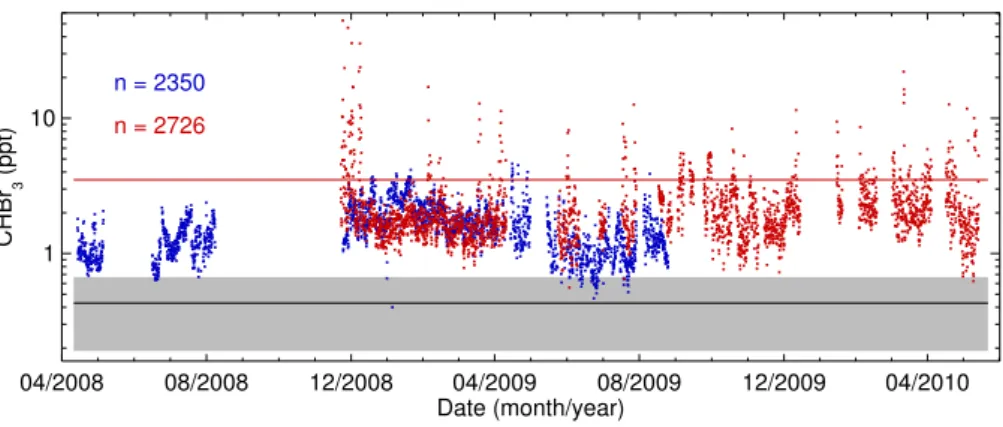
Robinson et al. (2014). The main features are summarised again here. The measurements were collected using Univer-sity of Cambridgeµ-Dirac instruments (Gostlow et al., 2010) at two locations in Sabah, Malaysia, and cover the period April 2008–May 2010. One instrument was located∼50 km from the nearest coast, at the Bukit Atur Global Atmospheric Watch site (elevation 426 m a.s.l.), within the Danum Val-ley Conservation Area. The second instrument was located at the coast, near the town of Tawau (elevation 15 m a.s.l.), and∼85 km south of Bukit Atur. The characteristics of the two measurement locations, and the quality of our data, are discussed by Robinson et al. (2014). Figure 1 shows the CHBr3 measurements, which have been averaged over 3 h

intervals to allow direct comparison with our model calcu-lations (see Sect. 3). The sampling rate of µ-Dirac means there are typically∼6 measurements in these 3 h windows. We will refer to these averaged data simply as “observa-tions”. Our CHBr3observations are a major enhancement to

(3)

04/2008 08/2008 12/2008 04/2009 08/2009 12/2009 04/2010 Date (month/year)

1 10

CHBr

3

(ppt)

n = 2350

n = 2726

Fig. 1.Observations of CHBr3, averaged over 3 h periods, from two locations in northern Borneo for April 2008 to May 2010. The blue data are from Bukit Atur, a rainforest location, and the red data are from Tawau, a coastal site. Theyaxis is logarithmic. The solid black line marks the “baseline” mixing ratio of 0.43 ppt assumed in the majority of the inversion experiments (see Sect. 3.2 for details). The shaded grey region indicates one standard deviation (±0.24 ppt) of the noise added to the observations (or equivalently the baseline, see Sect. 3.2.4). The solid red line, at 3.51 ppt, marks the 90th percentile of the coastal observations. The number of 3 h periods for which observations are available is noted to the top-left of the plot.

been collected during a cruise through the South China Sea (Mohd Nadzir et al., 2014) and near Borneo during the ap-proximately month-long SHIVA campaign (e.g. the aircraft data presented by Hossaini et al., 2013).

The CHBr3 mixing ratio at Tawau, on the coast, is

oc-casionally many tens of ppt, with ∼10 % of the observa-tions above∼3.5 ppt (a threshold marked by the red line in Fig. 1, and discussed with respect to our inversion calcula-tions in Sect. 5.1). Additional quantitative information can be found in the probability density functions, PDFs, presented by Robinson et al. (2014). While Robinson et al. (2014) do not identify a specific local cause of these high mixing ratios, previous studies have typically found such levels of CHBr3

when seaweed are nearby (e.g. Carpenter and Liss, 2000; Pyle et al., 2011). Aside from these periods, mixing ratios at Tawau are usually within the range 1–2 ppt. While there is often a small gradient in background mixing ratio between the coast and inland (again refer to the PDFs in Robinson et al., 2014), the majority of our inland data, and indeed many other observations apparently made away from strong CHBr3

sources (see Table 1–7 of Montzka and Reimann, 2011), also lie within this range.

Our data are used here to inform an inversion process, and so it is important to consider how observational uncertain-ties might impact our estimates of CHBr3emissions. First,

calibration errors might lead to biases in our observations, and in our subsequent emission estimates. A recent measure-ment inter-comparison (Jones et al., 2011) suggests that for CHBr3, discrepancies of∼10–20 % are possible. As this

un-certainty is likely to manifest itself as a bias, we attempt to assess its potential significance by repeating our inversion calculations with a range of “baseline” mixing ratios (see Sect. 3.2.2).

Another metric for measurement uncertainty is the preci-sion, which we define as the standard deviation of calibration peak heights divided by the mean height of such peaks (see also Robinson et al., 2014). Though the measurement preci-sion varied throughout the period covered, and was not iden-tical at the two locations, we use 7 % (i.e. 0.14 ppt, where the multi-site mean mixing ratio is 1.96 ppt) as a value rep-resentative of this type of uncertainty. The measurement pre-cision uncertainty is likely to be smaller than the uncertainty attached to the model calculations (Sect. 3.1) and to the as-sumptions inherent in the inversion method (Sect. 3.2), and is therefore incorporated into an overall uncertainty which is implemented as “noise” within the inversion process (see Sect. 3.2.4).

3 Modelling tools

In this section we first describe the atmospheric transport model we have used to calculate the immediate history of the air masses measured in Borneo. Section 3.2 introduces the associated inversion method used to estimate CHBr3

emis-sions, and discusses the assumptions and approximations this method requires.

3.1 NAME trajectory calculations

(4)

100 110 120 130 140 150 160 -10

0 10 20

3.2E-06 1.8E-05 1.0E-04 5.7E-04 3.2E-03 1.8E-02 1.0E-01 5.7E-01 3.2E+00

dilution (s m-1 )

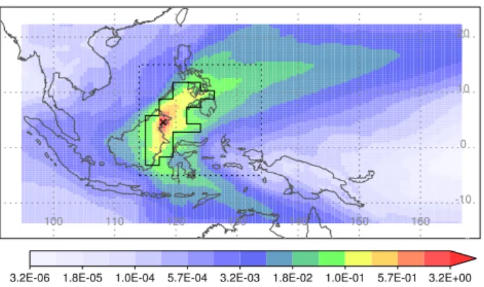
Fig. 2.The mean dilution matrix, averaged over backward trajec-tories released from both measurement locations, and over all 3 h periods for which observations are available at a particular mea-surement location. The black cross marks the average of the two proximate measurement locations. The grid covers∼95–165◦E, 13.5◦S–22◦N (128 by 96 grid cells). The units are s m−1and the colour scale is logarithmic. The solid black contour encloses the “fine” cells in the solution grid for which emission estimates are subsequently given. The dotted black box highlights the region plot-ted in Fig. 5 and 6.

latitude, though this was improved to∼0.35◦by∼0.23◦in February 2010. Within NAME a parameterisation of turbu-lence is also used (see Webster et al., 2003; Morrison and Webster, 2005).

NAME was used to calculate batches of 33 000 backward trajectories, released at random throughout each 3 h period for which CHBr3measurements were available at a

particu-lar location. In our measurement window there were a total of 2350 such periods at Bukit Atur, and 2726 at Tawau (see also Fig. 1). The trajectories were started randomly within an altitude range of 0–100 m. They ran for 12 days, and ev-ery 15 min the location of all trajectories within the low-est 100 m of the model atmosphere was recorded on a grid with the same resolution as the driving meteorological fields (always 0.5625◦ by 0.375◦). By counting only the “near-surface” trajectories a picture was built up of the areas from which surface emissions could have influenced the measured air masses during the previous 12 days.

In more detail, each trajectory is assigned an arbitrary mass, and the density of trajectories in each grid cell, in-tegrated over the 12 day travel time (units are g s m−3_{), is}

recorded. This density is then divided by the total mass of trajectories released (g), and multiplied by the area of the grid cell (m2). Physically, the resulting quantity (which has units of s m−1) can be considered the mean residence time in a particular grid cell, for all trajectories started in a particu-lar 3 h period, divided by the cell depth (100 m). Importantly, this quantity is the multiplicative factor by which emissions in a particular grid cell are diluted by the time they have trav-elled to a measurement location (see Eq. (1), and Manning

100 110 120 130 140 150 160

-10 0 10 20

Fig. 3.The solution grid, which contains cells of various sizes, and covers the same area as the dilution grid (Fig. 2). The “fine” grid cells (of size 1 by 1 and 2 by 2 dilution grid cells) are coloured in red/orange.

et al., 2011). So, a low dilution value means that few trajec-tories reaching Bukit Atur or Tawau have travelled through the boundary layer of a particular grid cell, and therefore that the impact of emissions from that grid cell on a measure-ment site will be correspondingly small. A grid of dilution values exists for the batch of trajectories started in each 3 h period. We will refer to the full three-dimensional (longitude-latitude-time) grid of dilution values as the “dilution matrix”. We approximate the effect of photochemical loss of CHBr3

by allowing the mass associated with each trajectory to de-cay with an e-folding time of 15 days (similar to the expected lifetime of CHBr3in the tropical lower troposphere, Warwick

et al., 2006; Hossaini et al., 2010; Liang et al., 2010). This has the effect of decreasing the dilution value in grid cells further from the measurement locations.

Figure 2 shows the time-averaged dilution matrix, calcu-lated over all 3 h periods for which observations are available at either location. It shows that the sites in Borneo are influ-enced by two prevailing wind directions, with northeasterly trade winds dominating during Northern Hemisphere winter, and southeasterlies during Northern Hemisphere summer. It also shows that large fractions of the plotted domain are crossed by relatively few trajectories (dilution values range over six orders of magnitude), and emissions in these re-gions are unlikely to appreciably affect our measurements. One consequence is that our emission estimates are made on a non-uniform grid, with larger grid cells used where the di-lution values are smaller (see Fig. 3 and the discussion later in Sect. 3.2.1).

(5)

height appear to be critical to determining atmospheric com-position (e.g. Pike et al., 2010), and Tawau, where a “sea breeze” circulation is common (Qian et al., 2013), may not be represented accurately in a global model such as the UM. Fi-nally, the rate at which air masses (i.e. trajectories) are mixed between the boundary layer and free troposphere in NAME will have a significant impact on our estimated emissions. Pyle et al. (2011) showed, and we reiterate in Sect. 4, that in the Maritime Continent this type of mixing seems to be weaker in NAME than in another model, p-TOMCAT. We attempt to assess the possible impact of these model-related uncertainties both by adding “noise” to our inversion pro-cess, and by adjusting the “baseline” CHBr3 mixing ratio

(see Sect. 3.2.4). 3.2 Inversion method

The inversion method employed here has been described by Manning et al. (2003, 2011), and is now known as the Inver-sion Technique for EmisInver-sion Modelling (InTEM). Using an optimisation process, the aim is to solve Eq. (1), and thereby locate the emission map, that can be multiplied by a NAME dilution matrix, to give modelled concentrations at a mea-surement site that most closely resemble the observed con-centrations (converted from volume mixing ratios using UM meteorological data).

emission(g m−2s−1)× dilution(s m−1) (1) = concentration(g m−3)

This calculation is conducted for each individual (source) grid cell: the emission in that grid cell, multiplied by the lo-cal value of the dilution matrix derived from the trajectory calculations, gives the contribution from those emissions to the simulated CHBr3concentration at a measurement

loca-tion (receptor). The sum over all source grid cell contribu-tions gives the total simulated CHBr3 concentration at one

particular time.

From Eq. (1) we obtain a spatially varying emission field. In solving this equation we assume the emissions are con-stant in time; clearly, when considering a compound with large natural emissions such as CHBr3, this is likely to be

a source of error in our estimates. In this section we discuss some of the other assumptions that are implicit in the method, which has typically been used to estimate emissions of com-pounds with lifetimes of years. So we also aim to highlight further uncertainties that are peculiar to our compound of in-terest, CHBr3, with its much shorter lifetime.

3.2.1 The solution grid

The time-averaged dilution matrix in Fig. 2 shows that air is most likely to travel towards our measurement locations from either the southeast or northeast, and more likely to travel over grid cells near to a measurement location than those fur-ther away. It is difficult to assess how the observations will be

affected by emissions from a particular grid cell if air seldom passes over it. Such grid cells are therefore grouped together using the method of Manning et al. (2011), into progressively larger squares of 2 by 2 cells, 4 by 4 cells and so on. As a result, the contribution to the observations from emissions in the new, grouped grid cell is larger or more frequent. This so-lution grid, containing grouped cells, is shown in Fig. 3, and is used for each of the inversion experiments in this study. We tested changing the resolution of the solution grid but found that such changes had a small impact on the results we present in Sect. 5.

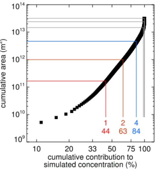
We can use the dilution matrix to assess the influence that emissions in solution grid cells of particular sizes might have on our measurements. If we assume that a tracer is emitted uniformly across our region of interest the dilution matrix can be used to derive a simulated concentration at both mea-surement sites (Eq. 1). Figure 4 shows the cumulative con-tribution to this modelled concentration when the individual dilution grid cells in Fig. 2 are added in turn (beginning with the largest dilution value). The red line (and label) shows that 44 % of this modelled concentration is due to emissions in solution grid cells of size 1 by 1, and that these cells cover an area of 1.65×1011m2 (∼0.1 % of the tropics). The orange (2 by 2), blue (4 by 4) and grey (8 by 8 to 32 by 32) lines in-dicate this relationship when solution grid cells of increasing size are also included in the calculation.

(6)

10 20 33 50 75 100 cumulative contribution to 109

1010 1011 1012 1013 1014

cumulative area (m

2)

1 44

2 63

4 84

simulated concentration (%)

Fig. 4.Each black square represents an individual grid cell in the di-lution matrix presented in Fig. 2 and, assuming a uniform emission throughout that area, shows the cumulative percentage of a simu-lated concentration at both measurement sites that is accounted for by adding emissions from that grid cell. The grid cells are counted successively, beginning with the grid cell containing the highest dilution value and finishing with the grid cell containing the low-est. This accumulated percentage is plotted against the surface area covered by the increasing number of grid cells considered. The lines relate to the different sized grid cells in the inversion solu-tion grid. The red line (and label) shows that 44 % of the hypothet-ical modelled concentration is caused by emissions in grid cells of size 1 by 1, which cover an area of∼1.6×1011m2. The orange (2 by 2), blue (4 by 4) and grey (8 by 8 to 32 by 32) lines indicate this relationship when solution grid cells of increasing size are also included in the calculation. For reference, the surface area between 20◦S–20◦N is 1.75×1014m2.

Table 1.The area (in m2) occupied when different maximum solu-tion grid cell sizes (see also Figs. 3 and 4) are considered, and the percentage of the tropics (20◦S–20◦N) this area covers. Then, for experiment D, the total emission from the selected grid (Egrid), and that emission extrapolated across the tropics (Etrop). Emission units are Gg CHBr3yr−1.

Max. size Area %trop Egrid Etrop

1 by 1 1.65×1011 0.09 % 0.17 180 2 by 2 9.94_×1011 0.57 % 1.28 225 4 by 4 4.64×1012 2.65 % 6.39 240

3.2.2 The “baseline”

Our backward trajectories can only be used to account for emissions occurring within the last 12 days. The contribution from earlier emissions therefore needs to be estimated, and subtracted from the observations. In the case of long-lived gases like CFCs, well-defined “baseline” mixing ratios can be observed at remote, unpolluted locations. Subtracting the

baseline mixing ratio from such observations should there-fore leave only pollution episodes caused by recent emis-sions. Here, though, where the compound of interest is short-lived, the concept of a baseline is less applicable. In addition, and in contrast to gases such as CFCs which have geograph-ically discrete sources, CHBr3is thought to be emitted over

much of the ocean (e.g. Butler et al., 2007). Therefore, in the Maritime Continent, air masses travelling in any direction to-wards the measurement locations may be subject to CHBr3

emissions. With a lifetime of ∼15 days though, it is also likely there is some contribution to the CHBr3observations

from emissions that occur more than 12 days previously, and that are therefore outside our solution grid.

In our experiments we use a constant baseline. This is a simplification, but there is no clear reason to select par-ticular air masses that might enable the construction of a time-varying baseline. In addition, our results are similar if a seasonally varying baseline is employed (not shown). In the majority of the inversions we use a baseline mixing ra-tio of 0.43 ppt. This is the mean contribura-tion from “rest of world” sources (i.e. those outside of a Southeast Asian do-main of similar size and location to our solution grid) to the modelled CHBr3 mixing ratio at Bukit Atur in a

multi-year p-TOMCAT simulation containing Pyle et al. (2011) emissions. Our choice of baseline mixing ratio is also close to the minimum observed value (0.40 ppt, see Fig. 1) so is consistent with an alternative definition based on the CHBr3

measurements. To examine how sensitive our emission esti-mates are to this choice, we conduct additional experiments in which the baseline is shifted up/down by one standard de-viation of the p-TOMCAT “rest of world” contribution to Bukit Atur (±0.19 ppt). These additional experiments also allow us to indirectly assess the possible impact of biases (e.g. in measurement calibration, or in the rate of modelled boundary layer to free troposphere mixing) on our estimated emissions.

3.2.3 Optimisation

The aim of the optimisation process, which is outlined in this section, is to find the emission distribution that provides the “best” match between the modelled time series, calculated using Eq. (1), and the observed time series. We use the nor-malised mean square error (NMSE, Eq. 2) as a cost func-tion to judge the strength of the agreement between the sim-ulated concentrations (m) and the three hourly average obser-vations (o), and it is this error that the optimisation process will seek to minimise. In Eq. (2),nis the sum of the number of observations at both measurement locations (2350 + 2726 = 5076, see Fig. 1).

NMSE = 1

n

n X

i=1

(mi−oi)2

¯

mo_¯ (2)

(7)

However, we obtain similar results if we use either the root-mean-square error or a cost function similar to that employed by Manning et al. (2011) with a mix of statistical measures.

If something is thought to be known about an emission distribution (for example, Stohl et al. (2009) assume zero oceanic emissions of selected anthropogenic halocarbons) then this knowledge can be incorporated into the cost func-tion. Again, the weighting (equivalently the confidence) as-signed to this so-called a priori information is subjective. As Manning et al. (2011) aim to generate an emission estimate that is entirely independent of “bottom-up” inventories, they do not use any a priori information. We believe that the char-acteristics of CHBr3 emissions are not known sufficiently

well to warrant the use of a priori information, with the ex-ception that there is little evidence for terrestrial sources. As such, rather than altering the cost function, our sole use of a priori information is to fix land emissions to be zero in some of our experiments.

The optimisation method used to minimise the cost func-tion is “simulated annealing”, so-called because of its con-ceptual similarity to annealing in metallurgy. The method is described in detail by both Kirkpatrick et al. (1983) and Press et al. (1986), and its application here is described by Man-ning et al. (2011). This particular approach is useful when, as is the case here, there are so many possible solutions to a problem that an exhaustive search for the optimum solution (i.e. the minimum cost) is impractical. The method therefore aims to find a solution that can not be improved upon sig-nificantly while using only limited computing time. In brief, the method investigates a solution space of possible emis-sion configurations. It iteratively searches the solution space to find the emission map that, after transformation to a sim-ulated concentration using the dilution matrix, most closely matches (as measured by Eq. 2) the observed time-series. We repeat each inversion experiment independently 25 times to obtain a range of emission estimates, with different solutions emerging due to the different noise added to the observations (Sect. 3.2.4) in each of the 25 repetitions.

3.2.4 “Noise” and uncertainty

As suggested in Sect. 2, there is a range of sources of uncer-tainty in the emission estimates based on Eq. (1). While we are able to quantify the uncertainty related to measurement precision with reasonable confidence (Sect. 2), the uncer-tainty attached to the model calculations and to the assump-tions inherent in the inversion method is more difficult to as-certain (see also Manning, 2011). In an attempt to account for these uncertainties a time series of “noise” (selected at random from a normal distribution with a mean of zero, and with a specified standard deviation) is added to the obser-vations (or equivalently, to the baseline which is subtracted from the observations, see Fig. 1).

For the inversion experiments presented in Sect. 5 we use a standard deviation of±0.24 ppt for the normally distributed

random numbers we add to the observations. This is the sum of two normal distributions: the first, with a standard devi-ation of 0.14 ppt, represents measurement precision uncer-tainty (see Sect. 2), and the second, with a standard deviation of 0.19 ppt, represents baseline uncertainty (Sect. 3.2.2). We have tried other forms of noise, including uniform distribu-tions, and different magnitudes, but find these changes have only a minor impact on our central emission estimates, and therefore on our conclusions. To reiterate a point made in Sect. 3.2.2, we also assess the importance of biases in both observations and modelling by adjusting the baseline mixing ratio.

3.2.5 Outline of inversion experiments

In Sect. 5 we will present results from six inversion ex-periments. The experiments are labelled A–F, and are sum-marised in Table 2. In experiments A–C we make use of dif-ferent subsets of the observations shown in Fig. 1, which en-ables us to explore the usefulness of observations with dif-ferent characteristics when used in this inversion method. In experiments D–F we consider the use of a priori information (i.e. fixing land emissions to zero), and vary the baseline to assess the possible impact of biases within our method.

In each experiment we use the dilution matrix described in Sect. 3.1, which is based on trajectories calculated over the entire measurement period. Recall that the mass associ-ated with these trajectories decays with a CHBr3-like 15 day

e-folding lifetime. We calculate emissions for the whole so-lution grid shown in Fig. 3, but will present results for only the “fine” cells, or size 1 by 1 and 2 by 2, in this grid. We use a constant baseline mixing ratio (typically 0.43 ppt, but shifted up and down in experiments E and F) and, in an at-tempt to account for our uncertainties, include normally dis-tributed random noise with a standard deviation of 0.24 ppt. The cost function is given in Eq. (2), and each experiment is repeated with a different application of noise 25 times.

4 Pseudo observations

Before using our observations to estimate emissions, we test the ability of our selected inversion method to find a “known” emission distribution. We generate “pseudo observations” using the dilution matrix and a “known” emission distri-bution (dimensionally, s m−1

×g m−2_s₋1_{= g m}₋3_{). Then,}

given only these pseudo observations and the dilution ma-trix, the inversion system should be able to iterate towards emissions close to those originally prescribed (e.g. Fig. 9 of Manning et al., 2011).

For our “known” emission distribution we use a re-gridded version of the CHBr3emissions reported by Pyle et al. (2011)

(8)

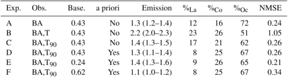
Table 2.A summary of various parameters used in, and results from, inversion experiments A–F. Observational constraint is provided by data collected at the inland site, Bukit Atur (BA), and the coastal location, Tawau (T). The coastal data is sometimes capped at the 90th percentile (T90). The baseline mixing ratio (units of ppt), and whether an a priori condition of zero emissions from land is employed, is also noted for each experiment. The table also summarises the CHBr3emission estimated by each experiment, which are discussed in Sect. 5. Emissions are listed for the “fine” solution grid cells (inside the solid black contour in Fig. 2, and in red/orange in Fig. 3). The grid cell-by-grid cell mean emission magnitude is given, with the range of the 25 separate solutions in parentheses. Emission units are Gg CHBr₃yr−1. The percentage of the total emission from land (La), coast (Co) and ocean (Oc) grid cells is also noted, with surface definitions taken from the UM land/sea mask. Finally, the cost function score (Eq. 2) for each experiment is noted.

Exp. Obs. Base. a priori Emission %La %Co %Oc NMSE

A BA 0.43 No 1.3 (1.2–1.4) 12 16 72 0.24

B BA,T 0.43 No 2.2 (2.0–2.3) 23 26 51 1.05

C BA,T₉₀ 0.43 No 1.4 (1.3–1.5) 17 21 62 0.26

D BA,T90 0.43 Yes 1.3 (1.1–1.4) 8 25 67 0.26

E BA,T₉₀ 0.24 Yes 1.4 (1.3–1.6) 9 26 65 0.21

F BA,T90 0.62 Yes 1.1 (1.0–1.2) 8 25 67 0.34

grid was identical to that derived from the real observations (Fig. 3), and a version of our “known” emissions, degraded to this non-uniform grid, is presented in Fig. 5b. Emissions in only the “fine” grid cells are shown in Fig. 5c (i.e. all larger grid cells are removed).

The average of 25 separate inversion solutions is shown in Fig. 5d (where the mean is calculated grid cell-by-grid cell), with only the “fine” grid cells shown in Fig. 5e. The statisti-cal agreement between the pseudo observations, which were not adjusted with noise, and the inversion-derived set of ob-servations is excellent (NMSE=0.0002). If we use the de-graded emissions (Fig. 5b) to generate the pseudo observa-tions, so that an exact solution is now possible, the statistical agreement is even stronger. The method is also able to quan-tify accurately the magnitude of regional emissions (the total emission from the plotted grid cells is given above each plot in Fig. 5).

Figure 5 also shows that our method is able to find nearby coastal emissions (that might be expected for CHBr3) if they

exist at our grid resolution, and if there is a clear signal in the observations. However, in more distant parts of the region, where the solution grid is coarser, coastal grid boxes (and emissions) cannot be separately resolved. We wish to retain information about the split between land, coast and ocean in our estimated emissions ahead of extrapolation to global scales in Sect. 5, so this problem provides additional motiva-tion for including only smaller grid cells in our definimotiva-tion of “fine” (see Sect. 3.2.1).

Consistent with the comparison of Pyle et al. (2011), these emissions developed for use in p-TOMCAT lead NAME to overestimate CHBr3 mixing ratios at both Bukit Atur

(ob-served mean, 1.55 ppt, and modelled mean, 2.04 ppt) and Tawau (2.32 ppt and 2.75 ppt). Pyle et al. (2011) reported a larger difference, and highlighted a discrepancy in the rate at which the boundary layer is vented in the two models, with this process less efficient in NAME. We discuss this type of model-to-model difference further in Sect. 6, but it

is certainly a significant, and difficult to quantify, source of uncertainty in the emission estimates we present in the next section.

5 Emission estimates

5.1 Local emissions

In this section we present emission estimates from six differ-ent inversion experimdiffer-ents, which are labelled A–F, and are summarised in Table 2. In Sect. 3.2 we discussed choices and assumptions that need to be made in the inversion method we employ; in general the results we present here are relatively insensitive to these assumptions.

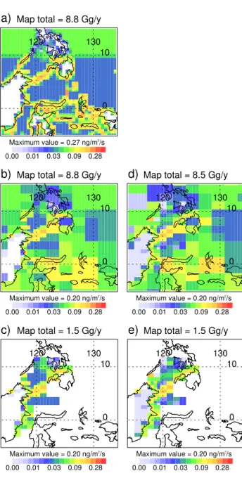
In experiment A only the observations from Bukit Atur, our inland measurement location, are used. As noted in Sect. 2, these data do not appear to have been influenced by nearby sources and therefore might be most suitable for estimating regional-scale emissions. As with the subse-quent experiments, the mean emission distribution in only the “fine” solution grid cells is shown in Fig. 6. The estimated emission magnitude from these “fine” cells is 1.3 Gg CHBr3yr−1, with the 25 individual solutions ranging

between 1.2–1.4 Gg CHBr3yr−1. The individual solutions to

experiment A containing the lowest and highest emission are shown in Fig. 7a and 7b; while the grid cell by grid cell de-tails of the distribution of emissions in these two solutions are somewhat different, the main features are consistent, with emissions found largely in the oceanic parts of the map, and much smaller over land.

Using the emissions from experiment A and the dilution matrix we now solve Eq. (1) to obtain simulated CHBr3

(9)

120 130

0 10 Map total = 8.8 Gg/y

0.00 0.01 0.03 0.09 0.28 Maximum value = 0.27 ng/m2

/s

120 130

/s

120 130

/s

120 130

/s

120 130

/s

a)

b)

c)

d)

e)

Fig. 5. (a)Shows CHBr3 emissions according to the Pyle et al. (2011) update to scenario 5 in Warwick et al. (2006) after re-gridding to match NAME’s grid. These emissions are used to cre-ate pseudo observations.(b)Shows these emissions degraded to the resolution of the solution grid (see Fig. 3), and(c)shows these de-graded emissions when only the “fine” solution grid cells are in-cluded. For comparison,(d)shows the mean solution of 25 inver-sions which use pseudo observations derived from the emisinver-sions in (a), and(e)shows this mean solution when only the “fine” grid cells are included. The total emission from the plotted grid cells is noted above each plot (units are Gg CHBr3yr−1), and the colour scale is exponential.

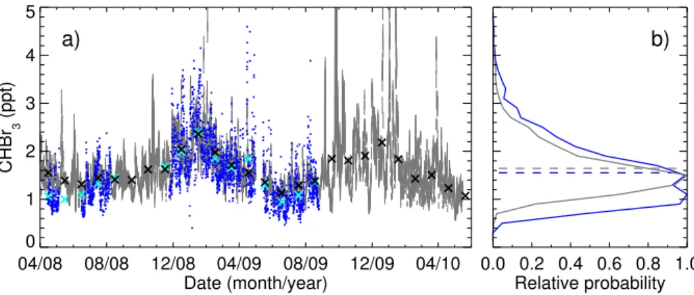
figure shows that, while the inversion-derived model time-series does not capture all the observed high frequency vari-ability, the monthly mean mixing ratios are in good agree-ment. Further, Fig. 8b demonstrates that the overall observed

120 130

0.00 0.01 0.03 0.09 0.28

Maximum value = 0.32 ng/m2

/s

120 130

0.00 0.01 0.03 0.09 0.28

Maximum value = 0.59 ng/m2

/s

120 130

0.00 0.01 0.03 0.09 0.28

Maximum value = 1.00 ng/m2_/s

120 130

0.00 0.01 0.03 0.09 0.28

120 130

0.00 0.01 0.03 0.09 0.28

120 130

0.00 0.01 0.03 0.09 0.28

A

B

C

D

E

F

Fig. 6. Estimated emissions of CHBr₃, for the “fine” grid cells (shades of red in Fig. 3). Experiment labels (see Table 2) are to the top-left of the plots, and in each case the mean of 25 sepa-rate solutions to the inversion process is shown. The total emission from the “fine” solution grid cells is noted above the plot (units are Gg CHBr3yr−1), and the colour scale is exponential.

mean mixing ratio, 1.55 ppt, is close to the modelled value, 1.64 ppt, and that the two timeseries contain similar charac-teristics of variability.

(10)

120 130

0.00 0.01 0.03 0.09 0.28

120 130

0.00 0.01 0.03 0.09 0.28

a) b)

Fig. 7.For experiment A, considering only the “fine” grid cells: (a)shows the individual inversion solution (one of 25) with the low-est low-estimated CHBr3emission, and(b)shows the individual solu-tion with the highest estimated CHBr3emission. As in Fig. 6, the total emission from the “fine” solution grid cells is noted above the plot (units are Gg CHBr3yr−1).

oceanic sources of CHBr3. However, emissions from coastal

grid cells are relatively small (16 %); as seaweed are thought to be a major CHBr3source in this region (Pyle et al., 2011)

this finding is perhaps unexpected.

Of course, the observations collected at Bukit Atur and Tawau are not independent of one another; they are the result of the same distribution of CHBr3emissions. So in

experi-ment B the observations from both sites are used in the same inversion. The total emission from the “fine” solution grid cells increases by ∼70 % to 2.2 (2.0–2.3 Gg CHBr3yr−1)

when we include these coastal data with, on average, higher mixing ratios. The distribution of emissions is also some-what different, with a larger percentage of emissions found both along coastlines (26 %, again see Table 2), which, given known CHBr3 sources, we might expect, and inland areas

(23 %), which we might not. The statistical agreement be-tween the observations and the modelled concentration is weaker (NMSE=1.05) than in experiment A. This differ-ence is largely caused by the occasional very high mixing ratios at the coast, which are presumably strongly influenced by emissions occurring very close to the Tawau site. These emissions will not be diluted according to the local value of the dilution matrix, and will therefore be difficult for the in-version method to account for.

In experiment C we attempt to remove the impact of these very local emissions. This is done by capping the coastal observations at the 90th percentile (3.51 ppt, marked with a red line in Fig. 1). All higher mixing ratios are set to this threshold. We accept that this is a crude approximation, but in support of our choice, we note that the 90th percentile of the coastal observations is very similar to the 99th per-centile mixing ratio observed inland at Bukit Atur (3.55 ppt), where we assume there are no local sources. We also re-peated this experiment using the 80th (2.65 ppt) and 95th

(4.75 ppt) percentiles as our threshold and found only small (∼10 %) differences in the total estimated emission magni-tude. The total emission from the “fine” grid cells is now 1.4 (1.3–1.5) Gg CHBr3yr−1, slightly higher than in

experi-ment A, but lower than experiexperi-ment B where the full range of coastal observations was included. Similarly, the distribution of emissions lies between experiments A and B, with 17 % from land, 21 % from coastal grid cells and 62 % from the ocean (Table 2). The statistical agreement is almost as strong as in experiment A (NMSE=0.26), confirming that the high-est CHBr3mixing ratios at the coast lead to the poorer

statis-tical agreement in experiment B.

In experiment D we repeat experiment C, but enforce an a priori condition of zero emissions from solution grid cells that contain only land. The inversion process remains free to attribute emissions to grid cells containing a mix of land and ocean. As CHBr3emissions are thought to be dominated by

oceanic sources it is encouraging that, according to our cost function, the solutions to experiments C and D are of equal quality (NMSE=0.26). Emissions from the “fine” solution grid cells total 1.3 (1.1–1.4) Gg CHBr3yr−1, a little lower

than without the “no land” constraint, and are now mostly distributed between the coast (25 %) and ocean (67 %). The remaining land emissions are placed in solution grid cells which contain both land and ocean, and so in reality are likely to be coastal emissions. In a similar way, some of the emis-sions attributed to land in experiments A, B and C are likely, in reality, to be due to coastal sources.

In the final pair of experiments, we repeat experiment D twice with a different baseline mixing ratio. In experiment E the baseline is lower than our best estimate, at 0.24 ppt. In F it is higher, at 0.62 ppt. As noted at the end of Sect. 3.2.2, these experiments allow us to assess the possible impact of biases, such as calibration errors, on our estimated emissions. As might be expected, the total emission from the “fine” grid cells in experiment D falls between the total with a lower baseline, 1.4 (1.3–1.6) Gg CHBr3yr−1, and the total with a

higher baseline, 1.1 (1.0–1.2) Gg CHBr3yr−1. The split of

emissions between land, coast and ocean is very similar in each of experiments D, E and F (Table 2, Fig. 6). The mean square error is also similar (within∼1 %), with the differ-ences in NMSE (Table 2) arising from the normalisation, which uses the mean modelled and mean observed mixing ratios after the baseline has been subtracted.

(11)

04/08 08/08 12/08 04/09 08/09 12/09 04/10 0

1 2 3 4 5

04/08 08/08 12/08 04/09 08/09 12/09 04/10 Date (month/year)

0 1 2 3 4 5

CHBr

3

(ppt)

0.0 0.2 0.4 0.6 0.8 1.0 Relative probability 0.0 0.2 0.4 0.6 0.8 1.0

Relative probability

a) b)

Fig. 8. (a)Shows both observed (blue) and modelled (grey) CHBr3 timeseries at Bukit Atur. The model data are presented as a range, between the smallest and largest mixing ratio simulated in a particular 3 h window using emissions from each of the 25 individual solutions to experiment A. Monthly mean observed (light blue crosses) and modelled (black crosses) mixing ratios are also presented.(b)Shows the probability density function for each of these timeseries, normalised using the respective maximum probabilities, and with mean mixing ratios indicated by the dashed lines.

5.2 Extrapolated emissions

We have focussed so far on one part of the Maritime Conti-nent, a region where transport from the troposphere to strato-sphere appears to be particularly efficient. However, it is also useful to scale our estimate across a larger area to enable a comparison with other global-scale estimates of CHBr3

emissions. Rather than extrapolating globally we wish to focus on the tropics (defined as 20◦S–20◦N), from which emissions are most likely to have an impact on stratospheric ozone, and for which our measurements may be most repre-sentative.

In our first extrapolation, we simply assume that emis-sions are uniform across the entire tropics, and extrapolate the “fine” emissions from the mean solution in experiment D using the ratio of surface areas. We include land in this calculation, but would obtain a similar answer using only the oceanic areas because, according to our land/sea mask, land comprises a similar percentage of these two domains: 27 % of the entire surface area between 20◦S–20◦N, and 32 % of our “fine” grid. This results in a best estimate of a source strength for the global tropics of 225 Gg CHBr3yr−1.

We choose experiment D because we believe that experi-ments A and B do not make the best use of our observa-tions, with A ignoring the coastal data altogether, and B be-ing too strongly influenced by emissions very close to our coastal instrument. We also prefer the assumption of zero land emissions (i.e. experiment D rather than C) because it is supported by the majority of observational evidence, and because we are able to obtain equally strong statistical agree-ment between model and measureagree-ment with or without this condition.

Next, we can examine how certain choices in our method affect our extrapolated emission magnitude. To begin, we use the estimates from experiment E (with a lower baseline) and

from experiment F (with a higher baseline) to obtain a pos-sible emission range related to the uncertainties in our in-version method. Extrapolating the maximum emission from the 25 individual solutions to experiment E and the mini-mum from experiment F yields a relatively narrow range of 180–280 Gg CHBr3yr−1. We can also consider the extent to

which our definition of “fine” grid cells impacts upon our ex-trapolation. If “fine” were defined with a maximum grid size of 1 by 1 then extrapolation gives a total tropical emission of 180 Gg CHBr3yr−1. Conversely, if the maximum grid cell

size were 4 by 4 the total tropical emission after extrapo-lation is 240 Gg CHBr3yr−1. These values are summarised

in Table 1. They also fall within the range given by experi-ments E and F, and show that our choice of “fine” grid has had a relatively small impact on our extrapolated emission magnitude.

As well as emission magnitudes, we also try to quantify the split between oceanic and coastal emissions. We continue to use the UM land/sea mask to determine which grid cells fall in to a particular category, focus on our central estimate, experiment D, and re-assign all land emissions to the coast. Within our “fine” grid, an emission of 0.86 Gg CHBr3yr−1

from the 174 ocean grid cells leads to a mean oceanic flux of 0.06 ng m−2s−1. Following the reassignment of land emis-sions, 0.42 Gg CHBr3yr−1 is emitted from the 86 coastal

grid cells, which leads to an identical mean coastal flux of 0.06 ng m−2s−1. Now, across the entire tropics, ∼73 % of the grid cells are ocean, and∼3 % match our definition of coast. Using the above fluxes, the resulting tropical emis-sion magnitudes are 247 Gg CHBr3yr−1from the ocean, and

11 Gg CHBr3yr−1from the coast. Their sum is broadly

sim-ilar to, but due to slightly different assumptions not equal to, the total emission of 225 Gg CHBr3yr−1 found above.

(12)

-6 -4 -2 0 2 elevation (km) 0.00

0.05 0.10 0.15 0.20

relative probability

Tropics (51820799)

Fine (291601)

0.284

-2 -1 0 1

log₁₀[chl-a] 0

5 0 5 0

(20514671)

(93186)

a) b)

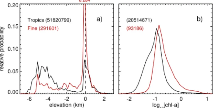
Fig. 9. (a)Shows a comparison of the distribution of surface eleva-tion in the tropics (20◦S–20◦N, in black) and in the “fine” grid cells (in red). The zero line, separating ocean from land, is marked with a dashed line. For the elevation data a bin size of 0.2 km is used, and the number of elevations in each classification is noted on the plot in parentheses.(b)Shows a similar plot for the chlorophylla

concentration measured by SeaWiFS. These data (original units are mg m−3) are log-transformed, and a bin size of 0.1 is used. Again, the total number of pixels contributing to each distribution is noted in parentheses.

the global ocean and the global coast; we return to this sub-ject in the next section.

For all these extrapolations it is reasonable to ask whether our region of focus around Borneo is representative of the tropics as a whole. To do this we briefly discuss two vari-ables, ocean depth and surface chlorophylla concentration, that have been related to CHBr3emissions in previous

stud-ies (e.g. Carpenter et al., 2009; Palmer and Reason, 2009; Ordóñez et al., 2012). Figure 9 shows PDFs for surface ele-vation (negative values give ocean depth) and chlorophylla

concentration for the whole of the tropics and for the “fine” grid cells. The elevation data have a horizontal resolution of ∼2 km, and are available from http://www.gebco.net/data_ and_products/gridded_bathymetry_data/. The chlorophylla

data have a horizontal resolution of∼9 km, and are from the satellite-borne Sea-viewing Wide Field-of-view Sensor (Sea-WiFS, available from http://daac.gsfc.nasa.gov/giovanni/); the PDFs are constructed using all available monthly mean products within our analysis period (i.e. November 2008– May 2010). Plot (a) shows that the “fine” grid cells contain proportionately more shallow water (depths of 0–200 m) and less deep ocean (depths∼5 km) than the tropics as a whole. In addition, plot (b) of this figure shows that the distribution of chlorophyllaconcentrations is shifted towards higher val-ues in the “fine” region than in the tropics (the tropical mean chlorophyllaconcentration is 0.20 mg m−3, while the corre-sponding value for the “fine” grid cells, 0.45 mg m−3).

While it has been suggested that, in broad terms, shallow water and high chlorophyll a concentrations may be asso-ciated with enhanced emissions of CHBr3 (e.g. Carpenter

et al., 2009; Palmer and Reason, 2009; Ordóñez et al., 2012), no robust relationships of this type have yet been

demon-strated. To illustrate, we have shown that coastal (similar to shallow water) emissions in our estimates are not stronger than non-coastal, or “open ocean” emissions. Further, our estimated emission distributions bear little resemblance to the distribution of either chlorophyll a, or of ocean depth (r2<0.05 when the elevation and chlorophylladata within the “fine” grid cells are degraded to the resolution of our emission estimates). As such we can only tentatively suggest that our extrapolations above, based upon estimates covering an area of relatively shallow and productive ocean, are more consistent with an upper limit for total tropical emissions.

We have also repeated the tropical emission extrapolation using an alternative definition of coast, based on ocean depth (elevation data as above). The distribution of land, coast (ocean shallower than 180 m, following Carpenter et al., 2009) and ocean within each grid cell was used to attribute emissions to each surface type. However, this new definition yielded similar results, and does not affect our conclusions. To illustrate, in the case of Experiment D, our original defi-nition of coast, based on the UM land/sea mask, led to 25 % of emissions in coastal areas, and 67 % in open ocean areas (see Table 2). Using this new definition the equivalent per-centages are 16 % and 72 %.

6 Summary and discussion

In this study we have described a new method to quantify CHBr3 emissions. For the first time, an inversion process

has been used to investigate systematically their distribution and magnitude. This process is informed by new long-term, high-frequency observations from Borneo, which are the first of their kind in the poorly sampled and convectively active Maritime Continent. We have examined how sensitive the estimated CHBr3emissions are to the characteristics of our

measurements, and to assumptions in the inversion method-ology.

We find that our local measurements of a short-lived com-pound like CHBr3, with presumed diffuse sources, are

over-whelmingly influenced by emissions from within a rela-tively small “footprint”, covering<1 % of the tropics (20◦S– 20◦N). This is also likely to be true of other CHBr3

measure-ments, and has the important implication that observations from a very large number of sites would be required to obtain global coverage. Within the footprint region our results are robust, with the various sensitivities considered often lead-ing to relatively minor changes, and emissions totalllead-ing 1.1– 1.4 Gg CHBr3yr−1. Even without a priori constraint these

emissions were largely distributed within oceanic grid cells, which is broadly consistent with expected sources due to the presence of either micro- or macroalgae.

An extrapolation of the flux calculated in experiment D results in a best estimate of tropical (20◦S–20◦N) emis-sions of 225 Gg CHBr3yr−1, with possible lower and upper

(13)

the baseline mixing ratio in experiments E and F. We note that the ocean in the “fine” region on which our extrapola-tions are based appears to be typically shallower, and more biologically productive, than the tropical average. Despite this, our estimate is slightly lower than those arrived at in recent global modelling studies. For the tropics defined as 20◦S–20◦N, these emissions include∼240 Gg CHBr3yr−1

(Liang et al., 2010),∼310 Gg CHBr3yr−1 (Warwick et al.,

2006, updated by Pyle et al. 2011) and∼300 Gg CHBr3yr−1

(Ordóñez et al., 2012). Our estimate, however, is somewhat higher than the recent “bottom up” estimate of Ziska et al. (2013), who used two different statistical methods to arrive at a tropical flux of ∼70–90 Gg CHBr3yr−1. We also

em-phasise that the spatial distribution of CHBr3 emissions in

our “fine” grid cells is not similar to the distribution of either chlorophyllaor ocean depth. Our study therefore echoes pre-vious findings: based on the two possible proxies we have ex-amined, no simple relationship that would enable a straight-forward physical parameterisation of CHBr3 emissions

ap-pears to exist.

Hossaini et al. (2013) have recently compared the impact of including the four other estimates discussed above in the same global model, and found that no single inventory al-lows a satisfactory match with observations in all locations. For the tropics, they found that the relatively low emissions of Ziska et al. (2013) provided the best match with the few available datasets. The paucity of tropical data, added to the fact that the different studies used different subsets of those data to construct their inventories, is likely to be one cause of the differing tropical emission values. Overall, the study of Hossaini et al. (2013) supports our finding, that using CHBr3

measurements from a relatively small number of locations makes constructing (or evaluating) a global emission inven-tory extremely difficult.

Our estimated emission distributions suggest that coastal CHBr3 sources, presumably related to seaweed, contribute

only a minor fraction of the total tropical emission. We cer-tainly believe that our observations from Tawau were af-fected by strong, nearby coastal CHBr3 emissions, but the

typical width of the coastal band that is affected by such sources is still not clear (see also Carpenter et al., 2009). The average CHBr3mixing ratios we observed inland were

lower than at the coast, and we also saw no elevated mix-ing ratios (i.e.>5 ppt) inland. This observed gradient occurs over a distance of∼50 km, which is well within a typical global model grid cell. The recent study of Leedham et al. (2013), which also focussed on the Maritime Continent, also suggests that the band of coastline directly influenced by macroalgae is likely to be rather narrow. Further investiga-tion of this type of gradient should be a priority because the global impact of coastal emissions is still poorly understood, and the best way to represent them in coarse global models is, therefore, still not clear. This is especially relevant for the Maritime Continent; it is conceivable that much of this region is influenced by coastal processes in some way.

Our examination of the “fine” grid cells near Borneo sug-gests a moderate (∼20 %) difference between the emissions that are most suitable for p-TOMCAT (see Fig. 5) and for NAME (i.e. our inversion solutions, Fig. 6). In comparison, the study of Pyle et al. (2011) reported differences of up to a factor of three in the CHBr3emissions inferred using these

two models, and for a similar area of the Maritime Continent. This may in part be because here we utilise year-round mea-surements, whereas Pyle et al. (2011) considered only a short period in which only southeasterly flow was sampled. An-other important difference is that this study uses coastal data, with higher average CHBr3mixing ratios, as a constraint. In

contrast the p-TOMCAT emissions reported by Pyle et al. (2011), and used here to generate our pseudo observations (Sect. 4), were constrained only by data collected inland at Bukit Atur. Further, those CHBr3mixing ratios observed at

Bukit Atur in mid-2008 have a mean of 1.21 ppt, which is substantially lower than the long-term (2008–2010) mean of 1.55 ppt for the dataset employed here.

We expect that underlying differences in the efficiency with which these models mix air (i.e. emissions) out of the boundary layer remain an important uncertainty in our emis-sion estimates (see also Robinson et al., 2012). The size of such systematic uncertainties could be explored by using me-teorological information from a different forecast centre to drive the NAME dispersion calculations (see Manning et al., 2011, who performed such a test and found little difference in mid-latitudes) and by using a different dispersion model, containing different, or additional parameterisations. Further studies assessing the characteristics of turbulence and re-lated tracer distributions in and immediately above the tropi-cal boundary layer, the influence of small-stropi-cale “sea breeze” type circulations, and the representation of these processes in dispersion models, are certainly required.

The limited constraint our new data provide on regional CHBr3emissions argues for an expanded network of

mea-surement locations in the Maritime Continent. The spac-ing of such a network should be similar to the size of the footprint region described here. We have made progress in this direction by recently starting to make measurements of CHBr3and other halocarbons at sites near Darwin, in

North-ern Australia, and in Bachok, on the East coast of Peninsu-lar Malaysia. Further, our two current measurement locations appear to be too close to distinguish between different re-gional scale influences on air mass composition. This is illus-trated by the very similar patterns of variability in our obser-vations of tetrachloroethene (C2Cl4), which appears to have

few local sources (see Robinson et al., 2014). In addition, the coastal observations used in this study are probably too close to strong local CHBr3sources to be used to estimate

(14)

across the coastal gradient would help to determine where such a level of influence occurs. We also emphasise that mea-surement locations should, as much as is possible in the Mar-itime Continent, avoid complicated terrain associated with prevailing smaller-scale circulations that are particularly dif-ficult to represent accurately in global meteorological mod-els.

Acknowledgements. M. Ashfold thanks the Natural Environment

Research Council (NERC) for a research studentship, and is grateful for support through the ERC ACCI project (project number 267760). N. Harris is supported by a NERC Advanced Research Fellowship. This work was supported through the EU SHIVA project, through the NERC OP3 project, and NERC grants NE/F020341/1 and NE/J006246/1. We also acknowledge the Department of Energy and Climate Change for their support in the development of InTEM (contract GA0201). For field site support we thank S.-M. Phang, A. A. Samah and M. S. M. Nadzir of Universiti Malaya, S. Ong and H. E. Ung of Global Satria, Maznorizan Mohamad, L. K. Peng and S. E. Yong of the Malaysian Meteorological Department, the Sabah Foundation, the Danum Valley Field Centre and the Royal Society. This paper constitutes publication no. 613 of the Royal Society South East Asia Rainforest Research Programme.

Edited by: W. T. Sturges

References

Aschmann, J., Sinnhuber, B.-M., Atlas, E. L., and Schauffler, S. M.: Modeling the transport of very short-lived substances into the tropical upper troposphere and lower stratosphere, Atmos. Chem. Phys., 9, 9237–9247, doi:10.5194/acp-9-9237-2009, 2009. Ayers, G. P., Gillett, R. W., Cainey, J. M., and Dick, A. L.: Chloride

and bromide loss from sea-salt particles in Southern Ocean air, J. Atmos. Chem., 33, 299–319, doi:10.1023/A:1006120205159, 1999.

Butler, J. H., King, D. B., Lobert, J. M., Montzka, S. A., Yvon-Lewis, S. A., Hall, B. D., Warwick, N. J., Mondeel, D. J., Ay-din, M., and Elkins, J. W.: Oceanic distributions and emissions of short-lived halocarbons, Global Biogeochem. Cy., 21, GB1023, doi:10.1029/2006GB002732, 2007.

Carpenter, L. J. and Liss, P. S.: On temperate sources of bromo-form and other reactive organic bromine gases, J. Geophys. Res.-Atmos., 105, 20539–20547, doi:10.1029/2000JD900242, 2000. Carpenter, L. J., Jones, C. E., Dunk, R. M., Hornsby, K. E., and

Woeltjen, J.: Air-sea fluxes of biogenic bromine from the tropical and North Atlantic Ocean, Atmos. Chem. Phys., 9, 1805–1816, doi:10.5194/acp-9-1805-2009, 2009.

Dvortsov, V. L., Geller, M. A., Solomon, S., Schauffler, S. M., At-las, E. L., and Blake, D. R.: Rethinking reactive halogen budgets in the midlatitude lower stratosphere, Geophys. Res. Lett., 26, 1699–1702, doi:10.1029/1999GL900309, 1999.

Gostlow, B., Robinson, A. D., Harris, N. R. P., O’Brien, L. M., Oram, D. E., Mills, G. P., Newton, H. M., Yong, S. E., and A Pyle, J.:µDirac: an autonomous instrument for halocarbon mea-surements, Atmos. Meas. Tech., 3, 507–521, doi:10.5194/amt-3-507-2010, 2010.

Gschwend, P. M., Macfarlane, J. K., and Newman, K. A.: Volatile Halogenated Organic-Compounds Released To Seawater From Temperate Marine Macroalgae, Science, 227, 1033–1035, doi:10.1126/science.227.4690.1033, 1985.

Hosking, J. S., Russo, M. R., Braesicke, P., and Pyle, J. A.: Mod-elling deep convection and its impacts on the tropical tropopause layer, Atmos. Chem. Phys., 10, 11175–11188, doi:10.5194/acp-10-11175-2010, 2010.

Hossaini, R., Chipperfield, M. P., Monge-Sanz, B. M., Richards, N. A. D., Atlas, E., and Blake, D. R.: Bromoform and dibro-momethane in the tropics: a 3-D model study of chemistry and transport, Atmos. Chem. Phys., 10, 719–735, doi:10.5194/acp-10-719-2010, 2010.

Hossaini, R., Chipperfield, M. P., Feng, W., Breider, T. J., Atlas, E., Montzka, S. A., Miller, B. R., Moore, F., and Elkins, J.: The contribution of natural and anthropogenic very short-lived species to stratospheric bromine, Atmos. Chem. Phys., 12, 371– 380, doi:10.5194/acp-12-371-2012, 2012.

Hossaini, R., Mantle, H., Chipperfield, M. P., Montzka, S. A., Hamer, P., Ziska, F., Quack, B., Krüger, K., Tegtmeier, S., At-las, E., Sala, S., Engel, A., Bönisch, H., Keber, T., Oram, D., Mills, G., Ordóñez, C., Saiz-Lopez, A., Warwick, N., Liang, Q., Feng, W., Moore, F., Miller, B. R., Marécal, V., Richards, N. A. D., Dorf, M., and Pfeilsticker, K.: Evaluating global emission in-ventories of biogenic bromocarbons, Atmos. Chem. Phys., 13, 11819–11838, doi:10.5194/acp-13-11819-2013, 2013.

Itoh, N. and Shinya, M.: Seasonal Evolution Of Bromomethanes From Coralline Algae (Corallinaceae) And Its Effect On At-mospheric Ozone, Mar. Chem., 45, 95–103, doi:10.1016/0304-4203(94)90094-9, 1994.

Jones, A., Thomson, D., Hort, M., and Devenish, B.: The U.K. Met Office’s Next-Generation Atmospheric Dispersion Model, NAME III, in: Air Pollution Modeling and Its Application XVII, edited by: Borrego, C. and Norman, A.-L., 580–589, Springer US, doi:10.1007/978-0-387-68854-1_62, 2007.

Jones, C. E., Andrews, S. J., Carpenter, L. J., Hogan, C., Hopkins, F. E., Laube, J. C., Robinson, A. D., Spain, T. G., Archer, S. D., Harris, N. R. P., Nightingale, P. D., O’Doherty, S. J., Oram, D. E., Pyle, J. A., Butler, J. H., and Hall, B. D.: Results from the first national UK inter-laboratory calibration for very short-lived halocarbons, Atmos. Meas. Tech., 4, 865–874, doi:10.5194/amt-4-865-2011, 2011.

Kirkpatrick, S., Gelatt, C. D., and Vecchi, M. P.: Opti-mization by Simulated Annealing, Science, 220, 671–680, doi:10.1126/science.220.4598.671, 1983.

Leedham, E. C., Hughes, C., Keng, F. S. L., Phang, S.-M., Malin, G., and Sturges, W. T.: Emission of atmospherically significant halocarbons by naturally occurring and farmed tropical macroal-gae, Biogeosciences, 10, 3615–3633, doi:10.5194/bg-10-3615-2013, 2013.

Levine, J. G., Braesicke, P., Harris, N. R. P., Savage, N. H., and Pyle, J. A.: Pathways and timescales for troposphere-to-stratosphere transport via the tropical tropopause layer and their relevance for very short lived substances, J. Geophys. Res.-Atmos., 112, D04308, doi:10.1029/2005JD006940, 2007.