www.atmos-chem-phys.net/8/5603/2008/ © Author(s) 2008. This work is distributed under the Creative Commons Attribution 3.0 License.
Chemistry
and Physics
A method for evaluating spatially-resolved NO
x
emissions using
Kalman filter inversion, direct sensitivities, and space-based NO
2
observations
S. L. Napelenok1, R. W. Pinder1, A. B. Gilliland1, and R. V. Martin2,3
1Atmospheric Sciences Modeling Division, Air Resources Laboratory, National Oceanic and Atmospheric Administration,
in partnership with the United States Environmental Protection Agency, 109 T. W. Alexander Drive, Research Triangle Park, NC 27711, USA
2Department of Physics and Atmospheric Science, Dalhousie University, Halifax, NS, Canada 3Harvard-Smithsonian Center for Astrophysics, Cambridge, MA, USA
Received: 18 January 2008 – Published in Atmos. Chem. Phys. Discuss.: 1 April 2008 Revised: 24 June 2008 – Accepted: 14 August 2008 – Published: 19 September 2008
Abstract. An inverse modeling method was developed and tested for identifying possible biases in emission inventories using satellite observations. The relationships between emis-sion inputs and modeled ambient concentrations were esti-mated using sensitivities calculated with the decoupled direct method in three dimensions (DDM-3D) implemented within the framework of the Community Multiscale Air Quality (CMAQ) regional model. As a case study to test the ap-proach, the method was applied to regional ground-level NOx emissions in the southeastern United States as
con-strained by observations of NO2 column densities derived
from the Scanning Imaging Absorption Spectrometer for Atmospheric Chartography (SCIAMACHY) satellite instru-ment. A controlled “pseudodata” scenario with a known so-lution was used to establish that the methodology can achieve the correct solution, and the approach was then applied to a summer 2004 period where the satellite data are available. The results indicate that emissions biases differ in urban and rural areas of the southeast. The method suggested slight downward (less than 10%) adjustment to urban emissions, while rural region results were found to be highly sensitive to NOxprocesses in the upper troposphere. As such, the bias in
the rural areas is likely not solely due to biases in the ground-level emissions. It was found that CMAQ was unable to predict the significant level of NO2in the upper troposphere
Correspondence to:S. L. Napelenok ([email protected])
that was observed during the NASA Intercontinental Chemi-cal Transport Experiment (INTEX) measurement campaign. The best correlation between satellite observations and mod-eled NO2column densities, as well as comparison to
ground-level observations of NO2, was obtained by performing the
inverse while accounting for the significant presence of NO2
in the upper troposphere not captured by the regional model.
1 Introduction
Regional air quality modeling has been used to develop con-trol strategies designed to reduce levels of pollutants such as ozone and particulate matter. Models have been used to assess our knowledge of atmospheric processes, including chemical and physical transformations of air pollutants, and to forecast air quality. More recently, results of regional mod-els have been integrated into epidemiological studies that aim to assess the health impacts of atmospheric pollutants (Knowlton et al., 2004). All of these applications rely on well quantified emission inputs. Emission inventories are tra-ditionally developed using a “bottom-up” approach that first estimates the levels of activity by various pollutant produc-ing sources, such as fossil fuel combustion by automobiles and the microbial activity in soils, and next, combines this information with activity-specific emission factors. Emis-sions of nitrogen oxides (NOx=NO+NO2) are of particular
the levels of ozone in the troposphere, lead to formation of nitric acid, which can be an important component of particu-late matter, and have a substantial impact on the levels of the hydroxyl radical that, in turn, determine the lifetime of many pollutants and greenhouse gases. The uncertainty in the es-timated emission levels of NOxhas been proposed to be as
high as a factor of two (Hanna et al., 2001).
Inverse modeling offers a “top-down” approach to eval-uating NOxemission inventories; where emission rates are
inferred by estimating possible changes that would result in the best comparison between predicted concentrations and observable indicators. While very few accurate surface ob-servations are available for NOx, space-based observations
of NO2columns offer a comparably rich dataset for inverse
modeling studies. Retrieval algorithms for NO2column
den-sities have been developed for several satellite instruments including Global Ozone Monitoring Experiment (GOME), Scanning Imaging Absorption Spectrometer for Atmospheric Chartography (SCIAMACHY), and more recently Ozone Monitoring Instrument (OMI) (Martin et al., 2002; Richter and Burrows, 2002; Beirle et al., 2003; Boersma et al., 2004; Bucsela et al., 2006). These data, as well as ground-based and other observations, have been used previously in in-verse modeling of “top-down” inventories on the global scale (Martin et al., 2003; M¨uller and Stavrakou, 2005), and more recently on the regional scale (Blond et al., 2007; Jaegl´e et al., 2005; Kim et al., 2006; Qu´elo et al., 2005; Konovalov et al., 2006; Konovalov et al., 2008; Wang et al., 2007). In this work, a method was developed for using NO2column
obser-vations to check for biases in the current emission inventories of NOxusing Kalman filter inversion. Regional scale
mod-eling was performed using the Community Multiscale Air Quality (CMAQ) model (Byun and Schere, 2006). The in-verse was driven by direct sensitivities that provided the spa-tial relationship between NOx emissions and NO2
concen-trations. Direct sensitivities were calculated using the decou-pled direct method in three dimensions (DDM-3D) (Yang et al., 1997). It is critical to resolve the spatial relationship be-tween emissions and concentrations in regional inverse mod-eling. On finer grid resolutions, transport lifetime can be shorter than chemical lifetime, as compared to coarser res-olutions of global models. Therefore, DDM-3D was invalu-able in this effort.
The inverse method was tested using a pseudodata sce-nario to evaluate the performance for a system with a known solution. After satisfactory performance, it was then applied to a summer-time episode in the southeastern United States using SCIAMACHY satellite observations of NO2 column
densities.
2 Method
2.1 Regional model and satellite observations
CMAQ (Byun and Schere, 2006) was used to simulate the concentrations of NO2as well as other pollutants in a domain
centered on the southeastern United States. The 36 km hori-zontal resolution domain with 14 vertical layers (Fig. 1) was nested within a larger domain covering the entire continental US that provided the boundary conditions. Meteorological fields were developed using the fifth generation mesoscale model (MM5) version 3.6.3 (Grell et al., 1995), and the emissions inputs were the result of the Sparse Matrix Opera-tor Kernel Emissions (SMOKE) version 2.0 (US-EPA, 2004) processing of the 2001 National Emissions Inventory (NEI) for use with the Statewide Air Pollution Research Center (SAPRC99) gas-phase chemical mechanism (Carter, 2000). The emissions included data from point sources equipped with continuous emissions monitoring systems (CEMs) that measure SO2 and NOxemission rates and other parameters
daily, mobile emissions processed by the Mobile6 model, and meteorologically adjusted biogenic emissions from Bio-genic Emission Inventory System (BEIS) 3.13 all specific for the year 2004. A more detailed description of these emission inputs is provided elsewhere (Gilliland et al., 2008).
Satellite observed NO2 columns were obtained from
SCIAMACHY (Bovensmann et al., 1999) on board the Eu-ropean Space Agency Environmental Satellite (ENVISAT). The data retrieval process is described in detail elsewhere (Martin et al., 2006). The horizontal resolution of a SCIA-MACHY footprint is 60 km by 30 km and it provides ob-servations at approximately 16:00 UTC in this domain. For comparison, satellite column observations and CMAQ grid values were paired in time and space from 1 June to 31 Au-gust 2004. The satellite column observations were mapped to the CMAQ grid resolution using area weighted averaging (Fig. 2c and d). During this three month period, satellite ob-servations were available for five days on average (range of three to ten days) over the modeling domain due to cloud events and satellite measurement schedule.
The modeling domain was subdivided into ten source re-gions including six southeastern metropolitan areas of At-lanta, Birmingham, Chattanooga, Macon, Memphis, and Nashville, as well as four larger rural areas approximately covering the states of Alabama, Georgia, Mississippi, and Tennessee (Fig. 1). The geographical extent of each metropolitan area was defined based on emission patterns.
A CMAQ-DDM-3D simulation for the summer months of 2004 provided the base-case fields of NO2 concentrations
and gridded sensitivities to NOx emissions from each
pre-defined source region. The vertical layers were aggregated to obtain column NO2values based on meteorological
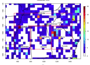
Fig. 1. Modeling domain covering the southeastern United States. Source region definitions are superimposed on a map of average sur-face layer NOxemissions at 16:00 UTC during the summer months
(JJA) of 2004. Source regions include urban areas of Atlanta, Birm-ingham, Chattanooga, Macon, Memphis, and Nashville and rural areas centered over Alabama, Georgia, Mississippi, and Tennessee. A four-cell wide border surrounds the source regions to minimize influence from the boundaries.
2.2 Kalman filter
To date, several different inverse methods have been ap-plied to adjust estimated emission rates of atmospheric pollu-tants based on observed data. These have included Bayesian based techniques (Deguillaume et al., 2007), data assimila-tion (Mendoza-Dominguez and Russell, 2000), and full ma-trix inversion such as the Kalman Filter (Hartley and Prinn, 1993; Gilliland and Abbitt, 2001), which was applied here. Kalman Filter is an optimization technique used to estimate discrete time series and states that are governed by sets of linear differential equations (Rodgers, 2000). In cases where the linearity assumptions are not always valid, such as atmo-spheric transport and chemistry systems, the technique can be applied iteratively. It has been tested previously for con-straining a variety of regional emissions including those of carbon monoxide (Mulholland and Seinfeld, 1995), ammo-nia (Gilliland et al., 2003), and isoprene (Chang et al., 1996). Kalman Filter is an attractive choice for this application be-cause it allows for weighting the solution based on the un-certainties of both observations and emission fields indepen-dently.
Full description of the Kalman Filter method is found elsewhere (Haas-Laursen et al., 1996; Gilliland and Abbitt, 2001). Briefly, it evolves an emissions vector,Ek+1,
accord-ing to the followaccord-ing:
Ek+1=Ek+Gk(χobs−χmod). (1) At iterationk+1, the emissions vector is altered based on the gain matrix,Gk, and the difference between the vectors of
Fig. 2. Total vertical NO2 column as(a) and (b) simulated by
CMAQ, (c)and (d) observed by SCIAMACHY, and (e) and (f)
simulated by CMAQ with upper-layer INTEX correction. The cor-rection is a uniform increase of 1.07×10¹⁵molecules cm−2based on the discrepancy between model predictions and measurements during the INTEX campaign of the upper troposphere. All show summer 2004 averages of days and locations with SCIAMACHY coverage. White areas represent regions with no SCIAMACHY ob-servations during the simulation period.
observations,χobs, and modeled values,χmod(the usual time subscripts are dropped for convenience, because only one time-step is considered in this application). The gain matrix is defined in terms of the partial derivatives of the change in concentration with respect to emissions,P, the covariance of the error in the emissions field,Ck, and the noise (including observation and model uncertainties),N, such that:
Gk=CkPT(PCkPT+N)−1 (2)
The covariance of error matrix also evolves with subsequent iterations according to:
Ck+1=Ck−GkPCk (3)
A variety of approaches have been used to estimate the initial covariance of error matrix,Ck=0, depending on
appli-cation of the technique. In this appliappli-cation,Ck=0was related
to the estimate of the normalized uncertainty in the emission, UE, according to the following:
Cmn,m6=n=
0.1·UE,m+UE,n
2 ·
Em+En 2
2
, (5)
for each subscripted (morn) element in the covariance of er-ror matrixC. The off-diagonal elements of the covariance of error matrix are difficult to estimate, and in this application were set to be a fraction (10%) of the average of the corre-sponding diagonals (Eq. 5).
Similarly, the noise matrix, Nt (Eq. 2) was initialized based on the estimated normalized uncertainties in the ob-servations,Uobsaccording to:
Nmm=Max
h
0.5·1015molecules·cm−2, (Uobs,m·χobsm )
i2 (6)
Nmn,m6=n=0.0 (7)
The value of Uobs, in this application, was set to 0.3
based on reported uncertainties in SCIAMACHY measure-ments (Martin et al, 2006). The minimum error value of 0.5×10¹⁵molecules cm−2is consistent with previous
satel-lite error estimates for NO2retrieval (Boersma et al., 2004)
and was imposed to prevent numerical instability. In this application, the noise matrix did not include an estimate of model uncertainties. An evaluation of model results re-vealed a clear systematic bias in NO2 column predictions
overwhelming any Gaussian type errors that would be in-cluded in the noise matrix. Possible sources of this bias and the approach of addressing it are presented later in Sect. 4. A detailed analysis of the dependence of the inverse on the assumption ofUE andUobsappears further.
2.3 Direct sensitivity analysis
To determine the relationship between emission rates from different source regions and resulting concentrations (P in Eq. 2), several methods have been used in the past. The sim-plest and the most widely used approach is the finite differ-ence method, where sensitivities are determined through a “brute force” difference in the pollutant concentration fields resulting from simulations of manually perturbed input pa-rameters. While the finite difference method is intuitive and straightforward to implement, it comes with a few disadvan-tages. It is often prone to numerical noise, dependent on the magnitude of the perturbation due to the nonlinear na-ture of pollutant responses to atmospheric processing, and cumbersome to implement for more than a few perturbations. Other methods for calculating sensitivities focus on comput-ing local derivatives about the nominal value of the sensitiv-ity parameter. These include the Green’s function method (Dougherty et al., 1979; Cho et al., 1987), the decoupled di-rect method (Dunker, 1981, 1984), and the adjoint method (Koda and Seinfeld, 1982; Sandu et al., 2003). The advan-tages of each of these depend largely on specific application, but the decoupled direct method in three dimensions (DDM-3D) (Yang et al., 1997) is often the most computationally
efficient for calculating direct sensitivities over the entire do-main for a large number of input parameters simultaneously. Sensitivity coefficients are defined as a change in pollutant concentrationsCi(x, t ) of speciesi, in spacex and timet, with respect to a perturbation in an input parameteraj(x, t), which relates to the unperturbed or nominal valueAj(x, t) according to:
aj(x, t )=(1+1εj)Aj(x, t )=εjAj(x, t ), (8) whereεj is the applied scaling factor. To separate the de-pendence of the sensitivity coefficients on the magnitude of aj(x, t) and to allow better opportunity for comparison, they are normalized byAj(x, t). The resulting first-order semi-normalized (with units identical toCi(x, t )) sensitivity coef-ficientSij(x, t) can then be described by:
Sij(x, t )=Aj(x, t )
∂Ci(x, t )
∂aj(x, t )
=Aj(x, t )
∂Ci(x, t )
∂(εjAj(x, t ))
=∂Ci(x, t ) ∂εj
(9) The decoupled direct method has been implemented and evaluated for several regional air quality models including CAMx (Dunker et al., 2002; Koo et al., 2007) and CMAQ (Cohan et al., 2005; Napelenok et al., 2006) and has been shown to accurately produce sensitivities of gaseous and par-ticulate species to input parameters that include emission rate, initial/boundary conditions, and chemical reaction rates. In this work, DDM-3D was used to spatially resolve the dependencies of pollutant concentration on emissions from each of the predefined source regions.
2.4 Integrated iterative inverse system
Sensitivities of NO2column concentrations were calculated
to emissions of NOxfrom each source region and integrated
into the Kalman Filter formulation according the following (time subscripts are, again, dropped for convenience): P(j, x)=SN O2,Ej(x)
Ej
, (10)
where matrix P (Eq. 2) is dimensioned by the number of source regions, allj, and the number of horizontal grid cells contained in any source region, allx. The sensitivity coeffi-cient is the response of NO2to emission reductions in each of
the source regions,j, normalized by the total emission rate in that source region,Ej. Each model grid cell contained by a defined source region was paired with the spatially matched averaged satellite observation to developχmodandχobs vec-tors in the inverse. In order to overcome the linearity as-sumptions in both the Kalman filter and the direct sensitiv-ity calculations, the inverse was calculated iteratively. The emissions field was adjusted according to the results of the inverse and the process was repeated until the ratio ofEk+1
Fig. 3. Outline of the presented inverse method. The itera-tive process is used to overcome nonlinearities in the relation-ship between NOx emissions and NO2 concentrations. The
con-vergence criteria (Ek+1=Ek+ε) can vary with application, but
0.001<|(Ek+1−Ek)/Ek|was used here.
3 Pseudodata analysis
In order to evaluate the inverse method, a controlled pseu-dodata experiment was designed for the modeling domain for 1 day – 1 August 2004. The goal was to determine per-formance of the inverse in a scenario where the solution is known. NOxground level emissions in each source region
between the hours 00:00 and 16:00 UTC were aggregated to approximate emissions that would contribute to concentra-tions of NO2 observed by the satellite overpass at
approx-imately 16:00 UTC. During the summer in the southeast, NOx has a relatively short lifetime, therefore, this time
in-terval captures the majority of emissions that would impact concentrations during the time of the satellite measurement. The aggregated emissions were arbitrarily adjusted by fac-tors ranging between 0.3 and 2.0. The resulting emissions vector became the a priori estimate for the inverse method. NO2column concentrations from the simulation using these
adjustments (χmod) were compared to NO2column
concen-trations in the base-case, which acted as pseudo observations (χobs). The Kalman filter method was then applied iteratively to recreate the base-case emissions.
As previously mentioned, Kalman filter requires an esti-mate of the initial covariance of the error in the integrated emissions estimates,Ct,0. In the pseudodata experiment, this
quantity was based on an estimate of the uncertainty in the emissions,UE, according to Eqs. (4) and (5). The normal-ized uncertainty in emissions,UE,j was assumed to be 2.0 for all source regionsj allowing for large departures from
Table 1. Regional Emission Adjustment for the pseudodata sce-nario. This arbitrary factor was applied to hourly emission rates in each region.
Source Region∗ Pseudodata Test Adjustment Factor Atlanta, GA 0.3
Birmingham, AL 1.8 Macon, GA 0.5 Memphis, TN 0.6 Nashville, TN 1.0 Chattanooga, TN 1.4 Mississippi 1.6 Alabama 0.7 Georgia 2.0 Tennessee 0.4
∗Urban area emissions are not included in the larger encompassing
regions.
a priori emissions estimates during the first iteration. The details on the sensitivity of this assumption are discussed later. Similarly, the noise matrix was based on the estimated uncertainties in the observations,Uobsaccording to Eq. (6).
Theoretically, the noise matrix,N, can account for both er-rors in observations, as it does here, and also erer-rors in the modeling system. However, in the case of the pseudodata test and the subsequent applications to satellite data, model uncertainties are assumed to be systematic and should have little bearing on the conclusions drawn from the application of the inverse. For the pseudodata test, uncertainty in “ob-servations” does not exist, because the system is perfectly controlled. Thus, the diagonals of the noise matrix,N, were set at the minimum value of 0.5 (1015molecules cm−2)2. An
important assumption in the development of this method is the fact that the disagreement between satellite observations and model outputs comes primarily from the emissions in-ventory. While the noise matrix allows the introduction of other errors (model errors, assumptions in satellite date re-trieval, etc.), it ultimately only limits how close to the ob-servations the iterative solution approaches. The pseudodata exercise avoids all other uncertainties and investigates the ro-bustness of the method when this assumption is strictly cor-rect. In the pseudodata test, the discrepancies between “ob-servations” and model results come only from the artificially introduced errors in the emissions inventory.
In application of the inverse method to the pseudodata sce-nario, the base case NOxemissions in each region were
re-produced within a few iterations. Particularly encouraging is the fact that both large increases (“Georgia”: 2.0) and large decreases (“Atlanta”: 0.3) in emissions were corrected effi-ciently. Consequently, the corresponding NO2column
con-centrations were also reproduced well (Fig. 4).
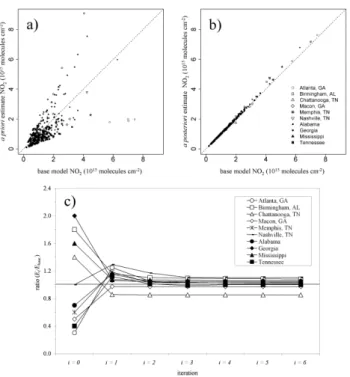
Fig. 4.Performance of the pseudodata analysis showing NO2 col-umn concentrations for(a) arbitrary adjusted emissions scenario and(b)inverse corrected emissions scenario (after six iterations), both compared to base case values (in 1015molecules cm−2), and
(c)the convergence toward base emissions from the perturbed start-ing point. Results are shown for 1 August 2004.
calculated as the adjustment factor to the emissions, Ek +1 / Ek , in the Atlanta source region resulting from varying UE and Uobs assumptions for k=0 in the pseudodata scenario. Larger uncertainties in emissions and smaller uncertainties in observations allow for larger adjustments in this and other source regions. The Atlanta source region requires an adjust-ment factor of 3.33 to return to the pre-perturbed inventory (to overcome a 0.3 perturbation).
The pseudodata analysis also offers the opportunity to test the response of the inverse to the assumptions in its eters. Assumptions where made for two important param-eters,UE andUobs(Eqs. 4 and 6). For the pseudodata test,
the uncertainty in observations was set to the minimum value (Eq. 6), while the uncertainty in the emissions was set to be 2.0. To test how the system behaves for a full range of these values would be computationally prohibitive. However, it is possible to test the response for just the first iteration of the Kalman Filter inverse with little requirement for CPU re-sources. It was already observed that the system converges on the correct solution in only a few iterations from starting with widely perturbed initial emission fields. The proxim-ity to the solution after one iteration should be indicative of the overall response to the assumptions. Thus, the first iter-ation of the inverse was tested at a range of values for both UE andUobs. As expected, larger uncertainties in emissions
Fig. 5. Sensitivity to inverse model assumptions ofUobsandUE
calculated as the adjustment factor to the emissions,Ek+1/Ek, in
the “Atlanta” source region resulting from varyingUE andUobs
assumptions fork=0 in the pseudodata scenario. Larger uncertain-ties in emissions and smaller uncertainuncertain-ties in observations allow for larger adjustments in this and other source regions. The “Atlanta” source region requires an adjustment factor of 3.33 to return to the pre-perturbed inventory (to overcome a 0.3 perturbation).
and lower uncertainties in observations allow for larger ad-justments to the emission fields in the case of the Atlanta source region (Fig. 5) and elsewhere. At the extreme highUE and extreme lowUobsthe adjustment is frequently
overesti-mated. In Atlanta, the emissions field required an adjustment factor of 3.3 to arrive back at the base emissions from the pseudodata perturbations (Table 1). However, factors higher than 4.0 were possible at extreme values of uncertainty as-sumptions. Further testing revealed that these overestima-tions were corrected in subsequent iteraoverestima-tions of the Kalman filter inverse.
The pseudodata case was also used to test the influence of the boundaries on the solution of the inverse. Since the domain is fairly small, influence from emissions outside the defined source regions, including boundary conditions, can be potentially problematic. Therefore, the source regions were “padded” with a border region (Fig. 1). Emissions from the border regions were assumed to not influence the defined source regions significantly. This assumption, as well as the ability of the border region to provide substantial enough dis-tance to negate boundary condition influences, was tested using DDM-3D sensitivities. Sensitivities of NO2 column
densities to boundary conditions of NOxand to emissions of
NOx from the border region were calculated and compared
Fig. 6.Fraction of total sensitivity of NO2column densities to(a)
NOxemissions from the “border” region(b)NOxboundary
condi-tions. NO2sensitivities to emission of NOxfrom(c)“Atlanta”,(d)
“GA”,(e)“Birmingham”, and(f) “AL” source regions are shown for comparison. The fraction for each grid cell as the ratio of the sensitivity from the source of interest and the total sensitivity from all source regions and the boundary conditions is expressed as:SN O2,EN Ox r·(
P10
r=1SN O2,E(N Ox)r+SN O2,BC(N Ox))−
1.
the defined source regions. It was found that both the border region and the boundary conditions had minimal influences (Fig. 6). The border region had the highest impact in the “MS” region where it accounted for under 25% of the to-tal sensitivity. In this same region, the boundary conditions also had the largest influence where they accounted for up to 30% of the total sensitivity in the southern portion of the re-gion. Overall, the border region provided reasonable separa-tion to neglect any impacts from the boundaries, mainly due to stagnant meteorological conditions common in southeast-ern summers and the consequently short chemical lifetime of NOxrelative to transport processes.
4 Case study: surface NOx emissions in the southeast United States
After encouraging results of the pseudodata analysis, the in-verse method was applied to the southeastern domain using SCIAMACHY observations for June, July, and August of
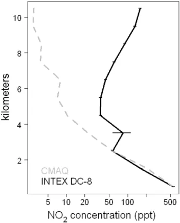
Fig. 7. Vertical distribution of NO2 concentrations observed by NASA INTEX DC-8 flights over the eastern United States com-pared to model predictions matched in space and time. Error bars denote 99% confidence interval of the mean, assuming that obser-vations are drawn from a normally distributed population. For more measurement details, see Bertram et al. (2007), Supporting Online Material, Fig. S6.
2004. The same emission source regions were used as in the pseudodata analysis (Fig. 1) and the emissions were again ag-gregated between the hours of 0:00 and 16:00. As was men-tioned previously, the 60 km by 30 km SCIAMACHY foot-prints were averaged down to the 36 km by 36 km CMAQ grid. To assure full coverage of the modeling domain by the infrequent and spatially varying observations, SCIAMACHY observations and modeling results sampled at the times and locations of available observations were averaged over the three summer months in the inverse. One of the major added complications in moving from a synthetic data test to an application with an independent dataset is the much greater impact on results from uncertainty stemming from the model’s ability to accurately reproduce natural condi-tions in the atmosphere. Regional transport models tend to under-predict NO2 concentrations in the upper troposphere
Table 2.Emission rates for each source region during the summer months (JJA) of 2004.
Source Region∗ a priori a posteriori posteriori – INTEX (tons/day) (tons/day) (tons/day) Atlanta, GA 513 482 435 Birmingham, AL 202 182 138 Macon, GA 154 68 73 Memphis, TN 129 118 106 Nashville, TN 112 113 80 Chattanooga, TN 55 101 89 Mississippi 572 859 212 Alabama 852 1718 782 Georgia 574 1171 364 Tennessee 1425 2533 1389
∗Urban area emissions are not included in the larger encompassing
regions.
altitudes. The under-prediction is easily visible from a com-parison of model predictions with vertical NO2profiles
ob-tained by aircraft measurements (Fig. 7). When compared with the average NO2vertical concentration profile estimated
from aircraft measurements taken during the NASA Inter-continental Chemical Transport Experiment (INTEX) (Singh et al., 2006; Bertram et al., 2007) over the eastern United States in the summer of 2004, our simulations under-predict by 1.07×10¹⁵molecules cm−2NO2in terms of column
den-sity (Fig. 7). This deficiency is of similar magnitude that has been reported by Konovalov et al. (2006), who proposed that the systematic negative bias of 8×1014cm−2 between satellite observation and their model simulation over Eu-rope was largely due to upper tropospheric NO2. To
un-derstand the sensitivity of the inverse solution to the upper layer NO2concentration uncertainty, the inverse method
us-ing SCIAMACHY observations was performed for two dif-ferent modeling realizations: a case where the model was used directly (Fig. 2a and b), and a case where the model-ing NO2column results were increased by spatially uniform
1.07×10¹⁵molecules cm−2based on INTEX observations of
the upper troposphere NO2concentrations during this time
period (Fig. 2e and f). For each case, the normalized uncer-tainty in the a priori emissions,UE, was set 2.0, which allows for large adjustments and follows the estimates of Hanna et al. (2001) for possible errors in NOxemissions. The
uncer-tainty in observation,Uobs, was set to 0.3 according to the
es-timates of Martin et al. (2006) of mean monthly uncertainty for SCIAMACHY observations of polluted regions.
As with the pseudodata analysis, only four iterations were necessary to obtain a solution. The inverse results using the base model confirm what is evident from a cursory exam-ination of the comparison between observed and modeled vertical columns of NO2 (Fig. 2a and b). In the southeast,
Fig. 8. Results of the inverse analysis showing(a)regionally av-eraged comparison of NO2column densities observed by
SCIA-MACHY and modeled by CMAQ with and without the INTEX cor-rection, as well as the comparison at four ground-based SEARCH sites: Atlanta (JST), Birmingham (BHM), suburban GA (YRK), and rural AL (CTR).
CMAQ predicts values that are too low in the rural regions while values in the urban centers are too high compared to SCIAMACHY observations. Accordingly, the inverse solu-tion was to dramatically increase emissions in the rural ar-eas and to slightly decrar-ease emissions in the urban arar-eas (Ta-ble 2). As a result of these adjustments, the correlation for the comparison between regional averaged observed and mod-eled NO2 columns improved fromR2=0.68 for the a priori
case to R2=0.89 (Fig. 8a). The inverse using INTEX ad-justed modeling results indicated that adding to the upper level background forced the emissions in most source regions lower (Table 2). Only the “Chattanooga” region required higher than base NOx emissions, because parts of
north-ern Georgia are highly sensitive to emissions there and still required upward adjustments. Furthermore, adding upper level NO2substantially reduced the bias in the comparison
and slightly increased the degree of correlation (R2=0.93) (Fig. 8a). Compared to areas of high surface emission den-sity, the inverse solution at rural areas is significantly more sensitive to upper layer NO2 concentrations. At rural
loca-tions, a large fraction of the column concentration is due to aloft emissions and long-range transport and less is due to surface emissions.
As the pseudo-data test and this case study demonstrate, the method developed here can improve the agreement be-tween modeled and observed NO2column densities. While it
is important to accurately simulate the NO2column density,
we are most interested in using this technique for improv-ing our simulation of surface air quality. However, the dis-crepancy in model and observed concentrations can be due to processes other than errors in emissions. Despite only pro-viding a column NO2density observed at a specific time, can
is useful as an independent check on the results and to de-termine the extent to which the results can be generalized to phenomena relevant to air quality.
NO2 concentrations at four Southeastern Aerosol
Re-search and Characterization Study (SEARCH) sites (Hansen et al., 2003) located in the domain were compared to both a posteriori modeling simulations averaged over the daytime concentrations for 1 June to 31 August 2004 (Fig. 8b). These sites measure NO2by photolytic conversion to NO followed
by chemiluminescence (Ryerson et al., 2000). The SEARCH network is designed to provide observations that are repre-sentative of either urban or regional conditions.
The INTEX corrected a posteriori emission estimates im-proved the simulated NO2 surface concentration at all four
surface monitoring sites. At the rural and suburban locations, the a posteriori emissions without the INTEX correction de-graded the quality of the simulation and caused an overesti-mate of the surface NO2concentration. This finding further
emphasizes the need for an accurate upper-troposphere NO2
simulation when applying this method to locations with low surface emission rates.
5 Conclusions and discussion
The Kalman filter inversion approach outlined here is a promising methodology for applying the increasingly rich dataset obtained by space-based measurements to regional air quality modeling. In the pseudodata analysis, the method algorithms and key assumptions were tested under ideal con-ditions. Problems with uncertain observations, spatial cover-age, and uncertain modeling results were largely eliminated. Under such conditions, the method performed extremely well and reproduced correct emission fields and corresponding NO2 concentrations in a few iterations. This suggests that
the method is theoretically sound.
One major obstacle of this and other inverse modeling ef-forts is the fact that the system is often mathematically ill-posed or is not constrained sufficiently to provide a unique and stable solution. However, this method offers some ad-vantages over other similar inverse modeling approaches. The use of direct sensitivities provides spatial and temporal resolution of the contributions to concentrations at any recep-tor in the domain from any and all source regions. Pollutant transport across source regions has been previously difficult to account for without direct sensitivities and often has been assumed to be negligible. This assumption is not unreason-able at the global scale with large source regions, but fails when finer spatial resolutions are introduced, because the transport lifetime of NOxis often shorter than the chemical
lifetime at the resolution of regional models. Similarly, sensi-tivity analysis also provides the opportunity to determine the degree of influence on concentrations from transport outside the defined source regions and from boundary conditions.
During the application to the southeastern United States a stable solution to the inverse was obtained for both cases: base model and INTEX adjusted model. The comparison of the results between the two cases suggests a much greater impact on upper layer processes in rural areas where NO2
concentrations aloft compose a larger fraction of the total column. In both cases, the results suggest very drastic ad-justments to the emissions inventory in some source regions, for example “Macon” and “GA”. While these results satisfy the mathematical model, which aims to minimize the dif-ferences between satellite derived observations and the re-gional model, their uncertainties should be explored further. Generally, in the rural areas, correct simulation of the upper troposphere NO2concentration is essential, because ground
sources of NO2are minimal. For urban areas, as ground level
NOx emissions increase, the importance of aloft processes
decreases, and, in a relative sense, approaches the error in the satellite product. However, in both low and high ground level source regions, the adjusted emissions improved ground level concentrations of NO2, as confirmed by the
dent SEARCH observations. This comparison to an indepen-dent data source builds confidence in a posteriori emission estimates and is a necessary check of the method, because Kalman Filter inversion attributes the difference between es-timates by the regional air quality model and satellite ob-servations solely to uncertainties in the emission inventories. The uncertainty in a posteriori emission estimates is mathe-matically reduced if the system converges on a stable solu-tion, but the solution must be verified by other means.
Other factors besides aloft sources influence the inverse results. In the “Macon” and “Mississippi” source regions, adjustments to the inventory are outside the specified uncer-tainty of the emissions inventory (factor of two). There, the differences between satellite observations and model results are likely to be a factor of other uncertainties besides those in the emissions inventory. These include insufficient spa-tial resolution, biases in the retrieval, and the representation of NOychemistry in CMAQ. In particular, the assumptions
used in the satellite retrieval algorithm for NO2columns can
impact the results of the inverse. The air mass factor cal-culation in the retrieval used here relied on relative vertical NO2profiles from a global model (GEOS-Chem) which
op-erates on a much coarser resolution (2◦ by 2.5◦) than the regional model. This inconsistency could introduce errors in the inversion. However, a better representation of free-tropospheric NO2 concentrations in CMAQ is needed
be-fore CMAQ NO2 profiles can be used for the AMF
calcu-lation. These issues will be explored further in the future applications of this method.
Summer-time sources of NOx in southeastern United
in regions with more densely located pollutant sources and for varied pollutant lifetimes.
Finally, the results of the inverse application need to be interpreted in the context of the emissions scenario. Only ground-level NOx emission fields were considered in this
study, under the assumption that elevated NOx come
pri-marily from point sources equipped with continuous emis-sion monitoring (CEM) devices and much more certainty. Sources of ground-level NOx vary by region. For instance,
the majority of biogenic NOx is emitted outside of the
de-fined urban regions as NO from soil, while in the urban cen-ters, mobile emissions are more important. The analysis pro-vided here does not provide the breakdown of how each sec-tor’s emissions should be adjusted; instead, the inverse was performed on the total. Sector specific adjustments are pos-sible to obtain and will be explored in the future. Another complication from using this approach of assigning emission quantities to source regions is the assumption that the daily emission profile is correct. Temporal dependencies are pos-sible with DDM-3D, and will be explored further.
Acknowledgements. The authors would like to thank Rynda Hud-man, Robin Dennis and Biswadev Roy for contributions and advice, statistical analysis assistance from Kristen Foley, and insightful comments from all reviewers. Work at Dalhousie University was supported by the Natural Sciences and Engi-neering Research Council of Canada. A portion of the research presented here was performed under the Memorandum of Un-derstanding between the US Environmental Protection Agency (EPA) and the US Department of Commerce’s National Oceanic and Atmospheric Administration (NOAA) and under agreement number DW13921548. This work constitutes a contribution to the NOAA Air Quality Program. Although it has been reviewed by EPA and NOAA and approved for publication, it does not necessarily reflect their policies or views.
Edited by: A. Richter
References
Beirle, S., Platt, U., Wenig, M., and Wagner, T.: Weekly cycle of NO2by GOME measurements: a signature of anthropogenic
sources, Atmos. Chem. Phys., 3, 2225–2232, 2003, http://www.atmos-chem-phys.net/3/2225/2003/.
Bertram, T. M., Perring, A. E., Wooldridge, P. J., Crounse, J. D., Kwan, A. J., Wennberg, P. O., Scheuer, E., Dibb, J., Avery, M., Sachse, G., Vay, S. A., Crawford, J. H., McNaughton, C. S., Clarke, A., Pickering, K. E., Fuelberg, H., Huey, G., Blake, D. R., Singh, H. B., Hall, S. B., Shetter, R. E., Fried, A., Heikes, B. G., and Cohen, R. C.: Direct Measurements of the Convective Recy-cling of the Upper Troposphere, Science, 315, 816–820, 2007. Blond, N., Boersma, K. F., Eskes, H. J., van der A, R. J.,
Van Roozendael, M., De Smedt, I., Bergametti, G., and Vautard, R.: Intercomparison of SCIAMACHY nitrogen dioxide obser-vations, in situ measurements and air quality modeling results over Western Europe, J. Geophys. Res.-Atmos., 112, D10311, doi:10.1029/2006JD007277, 2007.
Boersma, K. F., Eskes, H. J., and Brinksma, E. J.: Error analysis for tropospheric NO−2 retrieval from space. J. Geophys. Res.-Atmos., 109, D04311, doi:10.1029/2003JD003962, 2004 Bovensmann, H., Burrows, J. P., Buchwitz, M., Frerick, J., Noel,
S., Rozanov, V. V., Chance, K. V., and Goede, A. P. H.: SCIA-MACHY: Mission objectives and measurement modes. J. Atmos. Sci., 56(2), 127–150, 1999.
Bucsela, E. J., Celarier, E. A., Wenig, M. O., Gleason, J. F., Veefkind, J. P., Boersma, K. F., and Brinksma, E. J.: Algorithm for NO2 vertical column retrieval from the ozone monitoring in-strument. IEEE T. Geosci. Remote, 44(5), 1245–1258, 2006. Byun, D. W. and Schere, K. L.: Review of the governing equations,
computational algorithms, and other components of the Models-3 Community Multiscale Air Quality (CMAQ) modeling system, Applied Mechanics Reviews, 59, 51–77, 2006.
Carter, W. P. L.: Documentation of the SAPRC99 Chemical Mech-anism for VOC Reactivity Assessment, Air Pollution Research Center and College of Engineering, Center for Environmental Research and Technology, University of California, Riverside, CA, 2000.
Chang, M. E., Hartley, D. E., Cardelino, C., and Chang, W. L.: Inverse modeling of biogenic isoprene emissions, Geophys. Res. Lett., 23(21), 3007–3010, 1996.
Cho, S.-Y., Carmichael, G. R., and Rabitz, H.: Sensitivity analysis of the atmospheric reaction diffusion equation, Atmos. Environ., 12, 2589–2598, 1987.
Cohan, D. S., Hakami, A., Hu, Y., and Russell, A. G.: Nonlin-ear response of ozone to emissions: Source apportionment and sensitivity analysis, Environ. Sci. Technol., 39(17), 6739–6748, 2005.
Cooper, O. R., Stohl, A., Trainer, M., Thompson, A. M., Witte, J. C., Oltmans, S. J., Morris, G., Pickering, K. E., Crawford, J. H., Chen, G., Cohen, R. C., Bertram, T. H., Wooldridge, P., Perring, A., Brune, W. H., Merrill, J., Moody, J. L., Tarasick, D., Ned-elec, P., Forbes, G., Newchurch, M. J., Schmidlin, F. J., Johnson, B. J., Turquety, S., Baughcum, S. L., Ren, X., Fehsenfeld, F. C., Meagher, J. F., Spichtinger, N., Brown, C. C., McKeen, S. A., McDermid, I. S., and Leblanc, T.: Large upper tropospheric ozone enhancements above midlatitude North America during summer: In situ evidence from the IONS and MOZAIC ozone measurement network, J. Geophys. Res.-Atmos., 111, D24S05, doi:10.1029/2006JD007306, 2006
Deguillaume, L., Beekmann, M., and Menut, L.: Bayesian Monte Carlo analysis applied to regional-scale inverse emission mod-eling for reactive trace gases J. Geophys. Res.-Atmos., 112, D02307, doi:10.1029/2006JD007518, 2007
Dougherty, E. P., Hwang, J. T., and Rabitz, H.: Further develop-ments and applications of the Green’s function method of sen-sitivity analysis in chemical kinetics, J. Phys. Chem., 71, 1794– 1808, 1979.
Dunker, A. M.: Efficient calculation of sensitivity coefficients for complex atmospheric models, Atmos. Environ., 15, 1155–1161, 1981.
Dunker, A. M.: The decoupled direct method for calculating sensi-tivity coefficients in chemical kinetics, J. Chem. Phys., 81, 2385– 2393, 1984.
efficiency, Environ. Sci. Technol., 36(13), 2965–2976, 2002. Gilliland, A. B. and Abbitt, P. J.: A sensitivity study of the discrete
Kalman filter (DKF) to initial condition discrepancies, J. Geo-phys. Res., 106(D16), 17 939–17 952, 2001.
Gilliland, A. B., Dennis, R. L., Roselle, S. J., and Pierce, T. E.: Seasonal NH3emission estimates for the eastern United States
based on ammonium wet concentrations and an inverse method, J. Geophys. Res., 108(D15), 4477, doi:10.1029/2002JD003063, 2003.
Gilliland, A. B., Hogrefe, C., Pinder, R. W., Godowitch, J. M., Foley, K. L., and Rao, S. T.: Dynamic evaluation of regional air quality models: Assessing changes in O−3 stemming from changes in emissions and meteorology, Atmos. Environ., 42(20), 5110–5123, 2008.
Grell, G., Dudhia, J., and Stauffer, D.: A description of the fifth-generations Penn State/NCAR mesoscale model (MM5), NCAR Technical Note, NCAR/TN-398+STR, 1995.
Haas-Laursen, D. E., Hartley, D. E., and Prinn, R. G.: Optimiz-ing an inverse method to deduce time-varyOptimiz-ing emissions of trace gases, J. Geophys. Res., 101(D17), 22 823 – 22 831, 1996. Hanna, S. R., Lu, Z. G., Frey, H. C., Wheeler, N., Vukovich, J.,
Arunachalam, S., Fernau, M., and Hansen, D. A.: Uncertainties in predicted ozone concentrations due to input uncertainties for the UAM-V photochemical grid model applied to the July 1995 OTAG domain, Atmos. Environ., 35(5), 891–903, 2001. Hansen, D. A., Edgerton, E. S., Hartsell, B. E., Jansen, J. J.,
Kan-dasamy, N., Hidy, G. M., and Blanchard, C. L.: The southeastern aerosol research and characterization study: Part 1 – overview, J. Air Waste Manage., 53(12), 1460–1471, 2003.
Hartley, D. E. and Prinn, R. G.: Feasibility of determining surface emissions of trace gases using an inverse method in a three-dimensional chemical transport model, J. Geophys. Res., 98, 5183–5197, 1993.
Hudman, R. C., Jacob, D. J., Turquety, S., Leibensperger, E. M., Murray, L. T., Wu, S., Gilliland, A. B., Avery, M., Bertram, T. H., Brune, W., Cohen, R. C., Dibb, J. E., Flocke, F. M., Fried, A., Holloway, J., Neuman, J. A., Orville, R., Perring, A., Ren, X., Sachse, G. W., Singh, H. B., Swanson, A., and Wooldridge, P. J.: Surface and lightning sources of nitrogen oxides over the United States: Magnitudes, chemical evolution, and outflow, J. Geo-phys. Res.-Atmos., 112, D12S05, doi:10.1029/2006JD007912, 2007
Jaegl´e, L., Steinberger, L., Martin, R. V., and Chance, K.: Global partitioning of NOx sources using satellite observations:
Rel-ative roles of fossil fuel combustion, biomass burning and soil emissions, Faraday Discuss., 130, 407–423, 2005.
Kim, S. W., Heckel, A., McKeen, S. A., Frost, G. J., Hsie, E. Y., Trainer, M. K., Richter, A., Burrows, J. P., Peckham, S. E., and Grell, G. A.: Satellite-observed US power plant NOxemission
reductions and their impact on air quality, Geophys. Res. Lett., 33, L22812, doi:10.1029/2006GL027749, 2006
Knowlton, K., Rosenthal, J. E., Hogrefe, C., Lynn, B., Gaffin, S., Goldberg, R., Rosenzweig, C., Civerolo, K., Ku, J.-Y., and Kin-ney, P. L.: Assessing ozone-related health impacts under a chang-ing climate, Environ. Health Persp., 112(15), 1557–1563, 2004. Koda, M. and Seinfeld, J. H.: Sensitivity analysis of distributed
parameter systems, IEEE T. Automat. Contr.l, 27(4), 951–955, 1982.
Konovalov, I. B., Beekmann, M., Burrows, J. P., and Richter, A.: Satellite measurement based estimates of decadal changes in Eu-ropean nitrogen oxides emissions, Atmos. Chem. Phys., 8, 2623– 2641, 2008,
http://www.atmos-chem-phys.net/8/2623/2008/.
Konovalov, I. B., Beekmann, M., Richter, A., and Burrows, J. P.: Inverse modelling of the spatial distribution of NOx emissions
on a continental scale using satellite data, Atmos. Chem. Phys., 6, 1747–1770, 2006,
http://www.atmos-chem-phys.net/6/1747/2006/.
Koo, B., Dunker, A. M., and Yarwood, G.: Implementing the decou-pled direct method for sensitivity analysis in a particulate mat-ter air quality model, Environ. Sci. Technol., 41(8), 2847–2854, 2007.
Martin, R. V., Chance, K., Jacob, D. J., Kurosu, T. P., Spurr, R. J. D., Bucsela, E., Gleason, J. F., Palmer, P. I., Bey, I., Fiore, A. M., Li, Q., Yantosca, R. M., and Koelemeijer, R. B. A.: An improved retrieval of tropospheric nitrogen dioxide from GOME, J. Geophys. Res., 107(D20), 4437, doi:10.1029/2001JD001027, 2002.
Martin, R. V., Jacob, D. J., Chance, K., Kurosu, T. P., Palmer, P. I., and Evans, M. J.: Global inventory of nitrogen oxide emis-sions constrained by space-based observations of NO2columns,
J. Geophys. Res., 108(D17), 4537, doi:10.1029/2003JD003453, 2003.
Martin, R. V., Sioris, C. E., Chance, K., Ryerson, T. B., Bertram, T. H., Wooldridge, P. J., Cohen, R. C., Neuman, J. A., Swanson, A., and Flocke, F. M.: Evaluation of space-based constraints on global nitrogen oxide emissions with regional aircraft measure-ments over and downwind of eastern North America, J. Geophys. Res.-Atmos., 111, D15308, doi:10.1029/2005JD006680, 2006. Mendoza-Dominguez, A. and Russell, A. G.: Iterative inverse
mod-eling and direct sensitivity analysis of a photochemical air quality model, Environ. Sci. Technol., 34(23), 4974–4981, 2000. Mulholland, M. and Seinfeld, J. H.: INVERSE AIR-POLLUTION
MODELING OF URBAN-SCALE CARBON-MONOXIDE EMISSIONS, Atmos. Environ., 29(4), 497–516, 1995.
M¨uller, J.-F. and Stavrakou, T.: Inversion of CO and NOx emissions using the adjoint of the IMAGES model, Atmos. Chem. Phys., 5, 1157–1186, 2005,
http://www.atmos-chem-phys.net/5/1157/2005/.
Napelenok, S. L., Cohan, D. S., Hu, Y. T., and Russell, A. G.: Decoupled direct 3D sensitivity analysis for particulate matter (DDM-3D/PM), Atmos. Environ., 40(32), 6112–6121, 2006. Qu´elo, D., Mallet, V., and Sportisse, B.: Inverse modeling of NOx
emissions at regional scale over northern France: preliminary in-vestigation of the second-order sensitivity, J. Geophys. Res., 110, D24310, doi:10.1029/2005JD006151, 2005.
Richter, A. and Burrows, J. P.: Tropospheric NO2 from GOME measurements, Adv. Space Res., 29, 1673–1683, 2002. Rodgers, C. D.: Inverse methods for atmospheric sounding: theory
and practice, World Scientific Publishing Co. Pte. Ltd., 2000. Ryerson, T. B., Williams, E. J., and Fehsenfeld, F. C.: An efficient
photolysis system for fast-response NO2 measurements, J. Geo-phys. Res.-Atmos., 105(D21), 26 447–26 461, 2000.
Singh, H. B., Brune, W. H., Crawford, J. H., Jacob, D. J., and Rus-sell, P. B.: Overview of the summer 2004 intercontinental che mical transport experiment – North America (INTEX-A), J. Geo-phys. Res.-Atmos., 111, D24S01, doi:10.1029/2006JD007905, 2006.
Singh, H. B., Salas, L., Herlth, D., Kolyer, R., Czech, E., Avery, M., Crawford, J. H., Pierce, R. B., Sachse, G. W., Blake, D. R., Cohen, R. C., Bertram, T. H., Perring, A., Wooldridge, P. J., Dibb, J., Huey, G., Hudman, R. C., Turquety, S., Emmons, L. K., Flocke, F., Tang, Y., Carmichael, G. R., and Horowitz, L. W.: Reactive nitrogen distribution and partitioning in the North American troposphere and lowermost stratosphere, J. Geophys. Res.-Atmos., 112, D12S04, doi:10.1029/2006JD007664, 2007.
US-EPA: SMOKE v2.0 User’s Manual, http://www.smoke-model. org/version2/index.cfm, (last access: January 2008), 2004. Wang, Y. X., McElroy, M. B., Martin, R. V., Streets, D. G., Zhang,
Q., and Fu, T. M.: Seasonal variability of NOx emissions over east China constrained by satellite observations: Implications for combustion and microbial sources, J. Geophys. Res.-Atmos., 112, D06301, doi:10.1029/2006JD007538, 2007.