NO<sub><I>x</I></sub> lifetimes and emissions of hotspots in polluted background estimated by satellite observations

(1)

ACPD

15, 24179–24215, 2015

NO_x lifetimes and emissions of hotspots in polluted

background

F. Liu et al.

Title Page

Abstract Introduction

Conclusions References

Tables Figures

◭ ◮

Back Close

Full Screen / Esc

Printer-friendly Version

Interactive Discussion

Discussion

P

a

per

|

Discussion

P

a

per

|

Discussion

P

a

per

|

Discussion

P

a

per

|

Atmos. Chem. Phys. Discuss., 15, 24179–24215, 2015 www.atmos-chem-phys-discuss.net/15/24179/2015/ doi:10.5194/acpd-15-24179-2015

This discussion paper is/has been under review for the journal Atmospheric Chemistry and Physics (ACP). Please refer to the corresponding final paper in ACP if available.

NO

_x

lifetimes and emissions of hotspots

in polluted background estimated by

satellite observations

F. Liu1,2,3, S. Beirle3, Q. Zhang2, S. Dörner3, K. B. He1,2, and T. Wagner3

1

State Key Joint Laboratory of Environment Simulation and Pollution Control, School of Environment, Tsinghua University, Beijing 100084, China

2

Ministry of Education Key Laboratory for Earth System Modeling, Center for Earth System Science, Tsinghua University, Beijing 100084, China

3

Max-Planck-Institut für Chemie, 55128 Mainz, Germany

Received: 14 August 2015 – Accepted: 18 August 2015 – Published: 7 September 2015

Correspondence to: S. Beirle (steffen.beirle@mpic.de) and Q. Zhang (qiangzhang@tsinghua.edu.cn)

(2)

ACPD

15, 24179–24215, 2015

background

F. Liu et al.

Title Page

Tables Figures

◭ ◮

Back Close

Full Screen / Esc

Discussion

P

a

per

|

Discussion

P

a

per

|

Discussion

P

a

per

|

Discussion

P

a

per

|

Abstract

We present a new method to quantify NO_x emissions and corresponding atmospheric lifetimes from OMI NO₂observations together with ECMWF wind fields without further model input for sources located in polluted background. NO₂patterns under calm wind conditions are used as proxy for the spatial patterns of NO_xemissions, and the e_ffective

5

atmospheric NO_x lifetime is determined from the change of spatial patterns measured at larger wind speeds. Emissions are subsequently derived from the NO₂mass above background integrated around the source of interest.

Lifetimes and emissions are estimated for 17 power plants and 53 cities located in mountainous regions across China and the US. The derived lifetimes for

non-10

mountainous sites are 3.8_±1.0 h on average with ranges of 1.8 to 7.5 h. The derived NO_x emissions show generally good agreement with bottom-up inventories for power plants and cities. Global inventory significantly underestimated NO_x emissions in Chi-nese cities, most likely due to uncertainties associated with downscaling approaches.

1 Introduction 15

Nitrogen oxides (NO_x) are toxic air pollutants and play an important role in tropospheric chemistry as precursors of tropospheric ozone and secondary aerosols (Jacob et al., 1996; Seinfeld and Pandis, 2006). Power plants and cities with large vehicle popula-tions and intense industrial activities are significant anthropogenic emitting sources of NO_x. Accurate knowledge of NO_x emissions on urban scales is thus a critical factor

20

for accurate bottom-up emission inventories, which are important inputs for chemical transport models (CTMs) and for the development of mitigation strategies.

Bottom-up emission inventories depend on information of fuel consumptions and emission factors, which are subject to substantial uncertainties (Butler et al., 2008; Zhao et al., 2011). A significant improvement in accuracy of emission inventories for

25

(3)

ACPD

15, 24179–24215, 2015

background

F. Liu et al.

Title Page

Tables Figures

◭ ◮

Back Close

Full Screen / Esc

Discussion

P

a

per

|

Discussion

P

a

per

|

Discussion

P

a

per

|

Discussion

P

a

per

|

systems (CEMS). For example, in the US, under the 1990 Clean Air Act, power plant operators are required to install an automated data acquisition and handling system for measuring and recording pollutant concentrations from plant exhaust stacks and follow the monitoring regulations to ensure that the reported emission data is consistent and of high quality (Kim et al., 2009). For countries where reliable CEMS data is not

avail-5

able (like China), activity rates and emission factors can be adopted at plant-level to improve the accuracy of power plant emissions (e.g. Zhao et al., 2008; Liu et al., 2015). But developing emission inventories for individual cities with high accuracy faces enor-mous challenges, considering the lack of a complete and reliable database including fuel consumptions and emission factors at city level. Emissions at city level are often

10

forced to downscale regional emissions based on surrogates, like population density or industrial productivity, which however often just roughly reflect the magnitude and spatial distribution of urban emissions. Thus, independent emission estimates would be a desirable complement to validate and improve existing emission inventories.

The NO₂ tropospheric vertical column densities (TVCD, the vertically integrated

15

concentration in the troposphere) retrieved from satellite measurements provide valu-able global information on the spatio-temporal patterns of NO_x, including trends (e.g., Richter et al., 2005; Schneider and van der A, 2012; Hilboll et al., 2013), responses of NO₂ level changes to air quality control as well as economical and political factors (e.g., Duncan et al., 2013; Lelieveld et al., 2015), and temporal variations like weekly

20

cycles in NO₂ TVCDs (Beirle et al., 2003; Russell et al., 2010; Valin et al., 2014). In addition, the satellite NO₂ measurements allow quantifying NO_x emissions. In a pio-neering study (Leue et al., 2001), the downwind decay of NO₂ TVCDs in continental outflow regions was used to estimate a (constant) NO_x lifetime, which was then ap-plied to project global NO_xemissions from the measured mean NO₂TVCDs. Later on,

25

(4)

ACPD

15, 24179–24215, 2015

background

F. Liu et al.

Title Page

Tables Figures

◭ ◮

Back Close

Full Screen / Esc

Discussion

P

a

per

|

Discussion

P

a

per

|

Discussion

P

a

per

|

Discussion

P

a

per

|

the improved performance of model simulations with respect to in-situ measurements (e.g., Martin et al., 2006). However, the top-down inventories are usually determined at regional/global scale related to the spatial resolution of CTMs, while the spatial scales relevant for individual emission hotspots (power plants or cities) are not resolved. In addition, modelled lifetimes have large uncertainties (Lin et al., 2012) due to the highly

5

non-linear small-scale chemistry in urban areas, and are thus probably not appropriate for relating NO₂TVCDs to NO_x emission rates at city level.

With the launch of the Ozone Monitoring Instrument (OMI) (Levelt et al., 2006) with high spatial resolution, individual large sources like Megacities and power plants can be resolved. In a recent study, Beirle et al. (2011) averaged OMI NO₂ measurements

10

separately for di_fferent wind directions, thereby constructing clear downwind plumes which allow a simultaneous fit of the effective NOxlifetimes and emissions, without the

need of a chemical model. Similar lifetime/emission estimates have been performed recently by e.g. Valin et al. (2013), Lu et al. (2015) and de Foy et al. (2015). However, so far all studies assume that the source of interest can be considered as a “point

15

source”, which works well for isolated sources like e.g. the city of Riyadh, showing a high contrast against clean background with small and smooth TVCDs. However, for sources located in a heterogeneously polluted background, a modification of these methods is needed in order to account for the effect of interfering sources within small distances.

20

In this work, we present a new method for the quantification of NO_x lifetimes and emissions for power plants and cities located in polluted background. The mean OMI NO₂distribution for 2005–2013 is calculated separately for calm conditions as well as for di_fferent wind direction sectors according to ECMWF (European Center for Medium-range Weather Forecast) wind fields. The mean lifetime is derived from the change of

25

(5)

ACPD

15, 24179–24215, 2015

background

F. Liu et al.

Title Page

Tables Figures

◭ ◮

Back Close

Full Screen / Esc

Discussion

P

a

per

|

Discussion

P

a

per

|

Discussion

P

a

per

|

Discussion

P

a

per

|

2 Methodology

2.1 Satellite NO2data

We base this study on NO₂ TVCDs from the OMI tropospheric NO₂ (DOMINO) v2.0 product (Boersma et al., 2011), which is provided by the Tropospheric Emissions Mon-itoring Internet Service (TEMIS, http://www.temis.nl). OMI is a UV-VIS nadir-viewing

5

satellite spectrometer (Levelt et al., 2006) on board the Aura satellite (Celarier et al., 2008), launched in 2004. NO₂columns are derived from radiance measurements, us-ing the Differential Optical Absorption Spectroscopy (DOAS) algorithm (Platt, 1994). OMI provides daily global coverage with a local equator crossing time of approxi-mately 13:45 p.m. It detects radiance spectra by 60 across-track pixels with ground

10

pixel sizes ranging from 13 km×24 km at nadir to about 13 km×150 km at the outer-most swath angle (57◦). The 10 outermost pixels on both sides of the swath are ex-cluded in this study to limit the across-track pixel width<40 km. From June 2007, OMI has shown severe spurious stripes, known as row anomalies that are likely caused by an obstruction in part of OMI’s aperture (http://www.knmi.nl/omi/research/product/

15

rowanomaly-background.php). The a_ffected pixels are also excluded from the analysis. Only mostly cloud free observations (effective cloud fraction<30 %) are considered in this study.

Mean NO₂TVCDs over the US and China during “ozone season” (May–September) for 2005 to 2013 are calculated separately for calm (wind speed below 2 m s−1_{) and} 20

8 different wind direction sectors following the approach in Beirle et al. (2011). We focus on the ozone season to include the photochemically relevant months for ozone production (USEPA, 2014) and to exclude the winter data with larger uncertainties due to larger solar zenith angles, variable surface albedo (snow), and longer NO_x lifetime. Wind fields at a lat/long grid of 0.36◦ width are taken from the ECMWF ERA interim

25

(6)

ACPD

15, 24179–24215, 2015

background

F. Liu et al.

Title Page

Tables Figures

◭ ◮

Back Close

Full Screen / Esc

Discussion

P

a

per

|

Discussion

P

a

per

|

Discussion

P

a

per

|

Discussion

P

a

per

|

pixel center coordinates, and associated with the corresponding ECMWF wind fields interpolated in time.

2.2 Fitting procedure

In this section, we present a modified method compared to Beirle et al. (2011) for the determination of lifetimes and emissions for complex source distributions. The basic

5

idea is to use the measured NO₂spatial pattern under calm wind conditions as proxy for the distribution of NOx sources, instead of assuming a single point source.

Below, we (a) recap the fitting procedure of Beirle et al. (2011) and demonstrate that this method cannot be applied for multiple sources (Sect. 2.2.1), (b) describe the model function for the modified lifetime fit (Sect. 2.2.2), and (c) eventually explain how

10

emission rates are determined (Sect. 2.2.3).

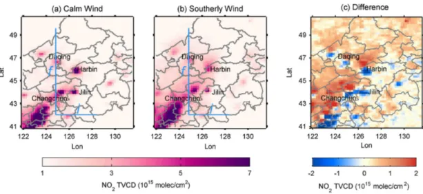
We select Harbin (45.8◦N, 126.7◦E), the capital of Heilongjiang province in China, with a population of about 6 million (city) to 10 million (greater area) inhabitants, to demonstrate our approach. Harbin is a typical city located in polluted background, surrounded by three other large NO_x sources (i.e. the cities of Daqing, Jilin and

15

Changchun) within ∼200 km radius. Figure 1 displays mean NO₂ TVCDs around Harbin for calm conditions (a), southerly wind (b) and their difference (c). The outflow plume of NO₂from Harbin is not as clear as that from isolated sources (e.g. Riyadh in Beirle et al. 2011), due to the interferences from surrounding sources. But the spatial pattern of their difference (Fig. 1c) still clearly reveals outflow patterns, consistent with

20

ECMWF wind fields.

In order to investigate the downwind plume evolution, 1-dimensional NO₂ “line den-sities”, i.e. NO₂ per cm, are calculated as function of distance for each wind direction sector separately by integration of the mean NO₂TVCDs (i.e. NO₂per cm2) perpendic-ular to the wind direction, as in Beirle et al. (2011).

(7)

ACPD

15, 24179–24215, 2015

background

F. Liu et al.

Title Page

Tables Figures

◭ ◮

Back Close

Full Screen / Esc

Discussion

P

a

per

|

Discussion

P

a

per

|

Discussion

P

a

per

|

Discussion

P

a

per

|

2.2.1 The original fitting procedure

In Beirle et al. (2011), a simple model functionM(x) (Eq. 1) was used to fit the observed line densities, which is composed of an exponential functione(x) (Eq. 2) describing the transport pattern and chemical decay, and a Gaussian functionG(x) (Eq. 3) accounting for di_fferent e_ffects causing spatial smoothing (e.g., the spatial extent of the source, the

5

OMI ground pixel size, or wind fluctuations).

M(x)₌E×(e⊗G)(x)+B (1)

e(x)=exp

−x−X

x0

forx≥X, 0 otherwise (2)

G(x)=_√1

2πσexp − x2

2σ2 !

(3)

Erepresents total emissions,Brepresents a constant background;X is the location of

10

the source (relative to the a priori co-ordinates of the site under investigation),x₀is the e-folding distance downwind; andσ is the SD ofG(x). The mean lifetime τ is derived from the e-folding distancex₀by division byw, the mean projected wind speed.

By this approach, emissions and lifetimes of NO₂are fitted simultaneously. In Beirle et al. (2011) it is applied for nine isolated hot spots exhibiting high NO₂ TVCDs over

15

a clean background within about 200 km. But it cannot be applied to hot spots sur-rounded by additional significant sources, like Harbin (Fig. 1), as by definition, the method can only represent a single “point source” convolved with a Gaussian func-tion. For instance, an additional source at 100 km with only 10 % of the emissions of the source under investigation causes a lifetime bias of_∼20 %, as the fit tries to

“ex-20

(8)

ACPD

15, 24179–24215, 2015

background

F. Liu et al.

Title Page

Tables Figures

◭ ◮

Back Close

Full Screen / Esc

Discussion

P

a

per

|

Discussion

P

a

per

|

Discussion

P

a

per

|

Discussion

P

a

per

|

2.2.2 New lifetime fitting procedure

We develop an alternative method accounting for emissions from multiple sources. The basic idea is to use the 1-dimensional NO₂patterns observed under calm conditions as proxy of emission patterns instead of assuming a single point source. Note that the 1-D pattern of line densities under calm conditions has to be determined along the same

5

(wind) direction, for which the line densities under windy conditions are determined. That means that in total eight 1-D line densities under calm conditions are determined for the eight wind directions. However, only directions with reasonable reliability are considered where mean NO₂line densities for both calm and windy conditions are well defined (i.e., gaps due to missing data are less than 10 % in the across-wind integration

10

intervali and less than 20 % in the fit interval in wind directionf). WithC(x) being the line density under calm wind conditions, we define the new model functionN(x) as:

N(x)₌a×[e⊗C] (x)₊b (4)

wheree(x) is again a truncated exponential function (Eq. 2 with X =0). The scaling factoraand offsetbare included to account for possible systemic differences between

15

windy and calm wind conditions (e.g. cloud conditions, vertical profiles, or lifetimes), which will be discussed in Sect. 3.1 in detail.

We perform a non-linear least-squares fit ofN(x) to the observed line densities with

a,b, andx₀as fitting parameters. We set the fit interval in wind directionf to 600 km (300 km in downwind direction, which corresponds to 3 times of the e-folding distance

20

for a lifetime of 5 h and a mean wind speed of 6 m s−1_{). The across-wind integration}

interval i is set to be half (300 km). f and i are indicated in Fig. 1a and b. The in-tervals are larger than those in Beirle et al. (2011), since not only the source under investigation, but also interfering sources have to be appropriately accounted for when comparing line densities of calm and windy conditions. We also perform fits with

dif-25

(9)

ACPD

15, 24179–24215, 2015

background

F. Liu et al.

Title Page

Tables Figures

◭ ◮

Back Close

Full Screen / Esc

Discussion

P

a

per

|

Discussion

P

a

per

|

Discussion

P

a

per

|

Discussion

P

a

per

|

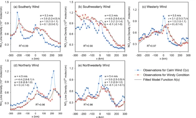
Figure 2a displays the observed line densities for calm (blue) and southerly winds (red) around Harbin, and the fitted model function N(x) (grey). Generally, N(x) de-scribes the observed downwind patterns well: the coefficients of determination (R2) between observation and fit are 0.96–0.99 for different wind directions, as shown in Fig. 2a–e.

5

Like in Beirle et al. (2011), the lifetimeτis derived by the ratio of the fitted e-folding distance and the mean wind speed1:τ=x₀/w. For Harbin,τis computed to be 3.9 h with a typical 95 % confidence interval (CI) of_±0.6 h for southerly winds. Averaging the fit results for all wind direction sectors with a good fit performance (i.e.R >0.9, lower bound of CI>0, and CI width<10 h,) yieldsτ=3.5 h with a SD of 0.6 h (Fig. 2), using

10

the fit residues as well as the CI ofτas inverse weights, as in Beirle et al. (2011).

2.2.3 New emission fitting procedure

The modified fitting function N(x) proved to be capable of gaining lifetime informa-tion even for complex source distribuinforma-tions. The interferences from multiple neighboring sources, which cannot be represented by a single-source Gaussian distribution, are

15

successfully described by the new model function usingC(x) as proxy for the spatial distribution of NO_x sources. However, in contrast to the previous fitting function M(x) in Beirle et al. (2011),N(x) does not contain the magnitude of NO_xemissions directly, but only the emission pattern represented by NO₂ under calm conditions. Thus, total NO_xemissions have to be estimated separately.

20

According to mass balance, the total mass of NO_x equals the emission rate times lifetime. Emissions can thus be derived in a three-step approach by (a) integrating observed TVCDs originating from the source of interest to calculate the total mass of

1

(10)

ACPD

15, 24179–24215, 2015

background

F. Liu et al.

Title Page

Tables Figures

◭ ◮

Back Close

Full Screen / Esc

Discussion

P

a

per

|

Discussion

P

a

per

|

Discussion

P

a

per

|

Discussion

P

a

per

|

NO₂, (b) scaling NO₂ to NO_x, and (c) division by the lifetimeτ, which was derived as described in the previous section.

a. Total NO₂mass

In order to quantify the total NO₂mass of the target source, the observed TVCDs

5

have to be integrated around the source, in which (1) interferences with neigh-boring sources have to be avoided and (2) a polluted background has to be ap-propriately accounted for. Thus, we base the estimation of the total NO₂mass on the mean TVCDs under calm conditions, to minimize interferences by advection. Again, we calculate line densities by integrating the NO₂TVCDs in “across-wind”

10

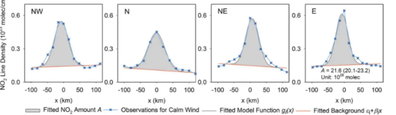
direction2, but for a smaller intervalv representing the spatial extent of megacities or urban centers, but exclude neighboring sources. Here we definev=40 km. We then perform a non-linear least-squares fit of a modified Gaussian functiong(x) to these line densities under calm wind condition, as illustrated in Fig. 3. The line densities integrated perpendicular to the di_fferent wind direction sectors are used

15

to constrain the fittedAing(x) :

g_i(x)₌A×_√ 1

2πσ_i exp − x2

2σ_i2

!

+ε_i+β_ix (5)

i represents the wind direction sector, i.e., Southeast–Northwest, South–North, Southwest–Northeast and East–West.σi is the SD of the Gaussiangi(x), andεi

andβi represent an offset and a possible linear gradient in the background field

20

respectively.The NO₂ amountA (in molecules) around the source on top of the (wind sector dependent) background is determined by fitting the functionsg_i(x) simultaneously for all available wind directions.

2

(11)

ACPD

15, 24179–24215, 2015

background

F. Liu et al.

Title Page

Tables Figures

◭ ◮

Back Close

Full Screen / Esc

Discussion

P

a

per

|

Discussion

P

a

per

|

Discussion

P

a

per

|

Discussion

P

a

per

|

The fit intervalhhas to be chosen to be larger thanv in order to allow for a mean-ingful fit ofg(x). We sethto 200 km for cities (see Fig. S2) and 100 km for power plants respectively. The fit interval thus potentially includes interfering sources. However, these interferences are in first order accounted for by the linear varia-tion of the background fitted in funcvaria-tiongi(x). Note that the fitg(x) is less sensitive

5

to interfering sources compared to the original fit of M(x) in Beirle et al. (2011), as lifetime is not involved here.

The small intervalv (40 km) excludes neighboring sources, but does not capture the full plume in across wind direction due to dilution. This e_ffect is corrected for by scalingAafterwards by a factorf(σ_i) based on the fitted plume widthσ_i:

10

f(σ_i)₌

20 km Z

−20 km

1

√

2πσ_iexp − x2

2σ_i2

!

/

∞ Z

−∞

1

√

2πσ_i exp − x2

2σ_i2

!

(6)

Note that we consider a larger interval (60 km for v and 300 km for h) for Pearl River Delta, which is a megalopolis covering nine prefectures over an area of about 56 000 km2.

The resulting emissions are rather insensitive with respect to modified settings

15

forv and h (see Supplement, Sect. 3). Again, fit results with poor performance (R <0.9, lower bound of CI<0, CI width>0.8_×A) are discarded.

b. Scaling NO₂to NOx

According to the typical [NO]/[NO₂] ratio of 0.32 under urban conditions at noon

20

(Seinfeld and Pandis, 2006), the total NO₂ mass is scaled by a factor of 1.32 in order to derive total NO_xmass following Beirle et al. (2011).

(12)

ACPD

15, 24179–24215, 2015

background

F. Liu et al.

Title Page

Tables Figures

◭ ◮

Back Close

Full Screen / Esc

Discussion

P

a

per

|

Discussion

P

a

per

|

Discussion

P

a

per

|

Discussion

P

a

per

|

For Harbin, the total mass (in terms of NO₂) is computed to be 33.2_×1028molec with a CI of 2.4×1028 molec. The total NO_x emissions derived for Harbin are 58.1 mol s−1.

2.3 Uncertainties

We define total uncertainties of the fitted lifetimes and emissions based on (a) the fit confidence intervals (CIs) and (b) the dependencies on the a priori settings as

investi-5

gated in sensitivity studies, analogue to the procedure described in Beirle et al. (2011). The CIs resulting from the least-squares fits of Eqs. (4) and (5) directly reflect the uncertainties of the derived lifetimes and emissions. In addition, the SDs of the fitted lifetimes for different wind direction sectors provide information on the consistency of the method. Beyond this, the results are also affected by the a priori choices of wind

10

fields, integration intervals etc. In particular, the calculation of line densities (a), wind fields (b), potential dependence of lifetimes on wind conditions (c) and fit errors (d) contribute to the uncertainties for bothτ and emissions, and uncertainties in the total NO₂mass fit (e), tropospheric NO₂TVCDs and the NO₂/NO_xratio (f) a_ffect the derived emissions. We define total uncertainties as the root of the quadratic sum of the above

15

mentioned contributions, which are assumed to be independent. We investigate the di_fferent sources of uncertainties contributing to the overall uncertainties of the derived lifetimes and emissions. Detailed sensitivity studies on the dependency of the fit results on the a priori settings are provided in Sect. 2 of the Supplement.

2.4 Bottom-up emission inventories 20

We use bottom-up emission inventories to pre-select promising sites and for a com-parison to the derived top-down estimates. We select inventories that provide up-to date, multi-year NO_x emissions at high spatial resolution and are widely used in the community. The following inventories are considered:

For power plants, we use the China coal-fired Power plant Emissions Database

25

(13)

ACPD

15, 24179–24215, 2015

background

F. Liu et al.

Title Page

Tables Figures

◭ ◮

Back Close

Full Screen / Esc

Discussion

P

a

per

|

Discussion

P

a

per

|

Discussion

P

a

per

|

Discussion

P

a

per

|

emission factors derived from various sources, and the US Emissions and Gen-eration Resource Integrated Database (eGRID) using emissions derived from con-tinuous emissions monitoring systems (available at http://www.epa.gov/cleanenergy/ energy-resources/egrid/) (USEPA, 2014). For cities, we use the Multi-resolution Emis-sion Inventory for China (MEIC: http://www.meicmodel.org) compiled by Tsinghua

Uni-5

versity and the global inventory of the Emissions Database for Global Atmospheric Research (EDGAR) v4.2 (EC-JRC/PBL, 2011) for the US.

For the comparison to the derived top-down estimates, a 8 year (2005–2012) aver-age from CPED and a 4 year (2005, 2007, 2009, and 2010) averaver-age from eGRID for the ozone season are used for power plants, of which the uncertainties are about 30 % (Liu

10

et al., 2015) for CPED and 10 % for eGRID (5 % arise from continuous emissions moni-toring systems (Gluck et al., 2003) and another 5 % arise from yearly variations in emis-sions after 2010), respectively. In addition, the mean emisemis-sions for the ozone season of the years 2005–2012 in MEIC and the mean annual emissions for the years 2005–2008 in EDGAR are used for cities, of which the uncertainty is estimated to be within a factor

15

of 1/2 and 2 according to the MEIC and EDGAR expert judgment of “medium magni-tude of uncertainty” (Olivier et al., 2002). The bottom-up urban emissions derived from regional/global inventories have larger uncertainties compared to power plant emis-sions, primarily arising from the low-resolution activity rates/emission factors at regional level, and the spatial allocation technique using surrogates to break regional-based

20

emission data down to cities. Furthermore, temporal coverage of bottom-up emissions is limited, inducing additional uncertainties. For instance, a decline in NO₂TVCDs from the years 2005–2008 to 2009–2013 with an average total reduction of 14_±9 % (mean

±standard variation) is detected for investigated US cities (Fig. S3). However, the most

recent year available in EDGAR v4.2 is 2008, which cannot reflect the recent decline

25

in NO_x emissions, thus overestimate the average emissions.

(14)

ACPD

15, 24179–24215, 2015

background

F. Liu et al.

Title Page

Tables Figures

◭ ◮

Back Close

Full Screen / Esc

Discussion

P

a

per

|

Discussion

P

a

per

|

Discussion

P

a

per

|

Discussion

P

a

per

|

metropolitan area for which the proposed top-down method is sensitive. Here, we de-fine this area as 40 km_×40 km, consistent with the considered intervalv in Sect. 2.2.3. For PRD, we consider a larger interval of 120 km×120 km.

2.5 Selection of investigated sources

For this study, we choose large power plants and cities across China and the US

5

as the pre-selected candidates, of which bottom-up emission information is avail-able from inventories described above. Power plants with NOx emission rates greater

than 10 Gg yr−1 (CPED/eGRID) are investigated. Power plants located in urban areas (100 km around city centers) are excluded by inspecting satellite imagery from Google Earth. The top 150 largest cities (rank in GDP/GDP per capita in 2013) in China and

10

the 47 large US cities selected for analyses in Russell et al. (2012) were also examined. To assure a good fit performance, the following criteria have been defined: (1) the signal of the source is strong, i.e., the mean NO₂TVCD in a circle of 100 km around the loca-tion center is larger than 1×1015molec cm−2; and (2) fit results with poor performance are discarded (see Sects. 2.2.2 and 2.2.3 for details). Table S2 of the Supplement

pro-15

vides a list of all sources under investigation which passed the criteria, including 24 power plants and 69 cities across China and the US.

2.6 Impact of topography

The accuracy of fitted lifetimes is highly dependent on the accuracy of the a priori wind directions (used for “sorting” the satellite NO₂ observations) and velocities (used for

20

converting x₀ into τ). However, accurate modelling of wind fields on small scales is challenging for large-scale models like ECMWF, which do not resolve urban scales. Consequently, wind fields might be biased in particular over complex mountainous ter-rain, related to the difficulties in resolving the characterization of small-scale orography in models (Beljaars et al., 2004).

(15)

ACPD

15, 24179–24215, 2015

background

F. Liu et al.

Title Page

Tables Figures

◭ ◮

Back Close

Full Screen / Esc

Discussion

P

a

per

|

Discussion

P

a

per

|

Discussion

P

a

per

|

Discussion

P

a

per

|

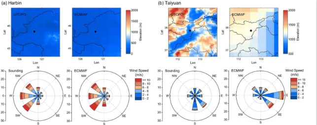
We investigate the impact of topography by comparing ECMWF wind fields to 2005– 2013 sounding measurements assembled by University of Wyoming (http://weather. uwyo.edu/upperair/sounding.html), and illustrate it for the cities of Harbin (plain ter-rain) and Taiyuan (mountainous city in Shanxi, China) in Fig. 4. In the top panels, to-pography used by ECMWF is compared to the topographic data from the 30 arc sec

5

global land topography “GTOPO30” archived by the US Geological Survey (avail-able at https://lta.cr.usgs.gov/GTOPO30, rescaled to 0.05◦). Topographic variations are smeared out significantly by the topographic model used in ECMWF, due to its coarser spatial resolution of 0.36◦. The bottom panels show statistics for wind vectors below 500 m during daytime (12:00) and nighttime (00:00) from both ECMWF and the

sound-10

ing measurements. The frequency distribution of wind directions (in 45◦ bins) shows a very good agreement in Harbin, but not in Taiyuan: here southerly flows dominate according to sounding measurements, while easterly winds dominate in ECMWF.

We compared wind fields for cities where the fits work properly (Table S2) and the sounding measurements are available simultaneously, as presented in Table S3. For

15

a mountainous city where the elevation in ECMWF contrasted sharply with that in GTOPO, Denver for instance, the correlation in wind speeds between ECMWF and sounding measurements is found to be much lower than for a non-mountainous city like Harbin.

Note that an error in a priori wind direction generally leads to a misclassification

20

during the sorting of the satellite data. In such a case, the assumed wind component in direction of the sector is higher than the actual projection; if, for instance, the true wind would be 5 m s−1 from north, but the model wind is 5 m s−1 from east, the case is classified as easterly, while the actual easterly wind is 0. This leads to a systematic high biased projected wind speed in Eq. (4), and thus a low biased lifetime. Thus,

25

mountainous sites often yield very low lifetimes (Table S2).

(16)

ACPD

15, 24179–24215, 2015

background

F. Liu et al.

Title Page

Tables Figures

◭ ◮

Back Close

Full Screen / Esc

Discussion

P

a

per

|

Discussion

P

a

per

|

Discussion

P

a

per

|

Discussion

P

a

per

|

larger than 250 m. A total of seven power plants and 16 cities are rejected based on the criteria, as listed in Table S4. Seven sites in Table S3 fulfill this criteria and 6 of them present low correlation (r2<0.5) in wind speeds between ECMWF and sounding measurements.

3 Results and discussions 5

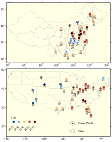
We applied our modified method for determining NO_x lifetimes and emissions to 17 power plants and 53 cities across China and the US (see Fig. 5), which passed the criteria defined in Sects. 2.5 and 2.6. Some strong hotspots are not included as they are mountainous, e.g. Denver or Salt Lake City.

3.1 Lifetimes 10

Figure 6 illustrates the fitted NO_xlifetimes for power plants and cities across China and the US, which demonstrates the wide applicability of the modified method developed in this study. The derived lifetimes in “ozone season” (May–September) are 3.8±1.0 h on average with ranges of 1.8 to 7.5 h. These values are in agreement to previously reported NO_x lifetimes (e.g., Beirle et al., 2004, 2011; Schaub et al., 2007; Valin et al.,

15

2013) and correspond to a mean OH concentration of the order of 107molec cm−3

(Valin et al., 2013), which is a realistic number for a polluted urban plume around noon (e.g., Kramp and Volz-Thomas, 1997; Dillon et al., 2002; Hofzumahaus et al., 2009). For the investigated sites, average lifetime for Power Plants (3.5 h) was found to be slightly shorter than for cities (3.9 h). Individual lifetimes have uncertainties of about

20

60 %. But, still, Fig. 6 indicates that lifetimes are not completely random, but show systematic spatial patterns. We could not unambiguously relate the variability of NO_x lifetime to a driving parameter, like surface elevation, mean wind characteristics, or lat-itude. But there is a tendency that NO_xlifetime is longer in heavily polluted regions with higher NO₂TVCDs, e.g., eastern China and eastern US: the mean NO₂TVCD for the

(17)

ACPD

15, 24179–24215, 2015

background

F. Liu et al.

Title Page

Tables Figures

◭ ◮

Back Close

Full Screen / Esc

Discussion

P

a

per

|

Discussion

P

a

per

|

Discussion

P

a

per

|

Discussion

P

a

per

|

ozone season in a circle with a radius of 100 km around sources with lifetimes over 5 h is 6.3_×1015molec cm−2, while it is only 1.3_×1015molec cm−2 for sources with lifetime less than 2 h. This finding might be related to nonlinear NOx chemistry, resulting in

a positive correlation between NO_xlifetimes and NO₂TVCDs when the concentration of NO_x is high (Valin et al., 2013). However, we also find that a high NO_x

concentra-5

tion does not necessarily correspond to a long lifetime, and the correlation between NO₂ TVCDs and NO_x lifetime is rather low (r2=0.22), probably due to the complex NO_xchemistry, which is as well a_ffected by meteorological and chemical variability, like variations in UV flux, water vapor and VOC levels.

The proposed method estimates the mean lifetime basically from the change of NO₂

10

patterns for windy vs. calm conditions. Valin et al. (2013) report on a dependency of the NOx lifetime on wind speed, with generally shorter lifetimes for higher wind speed. In

addition, other factors, like the satellite’s sensitivity (affected by e.g. cloud properties or the vertical NO_xprofile) and the NO₂background might change systematically between calm and windy conditions. In the fitted model function N(x), a scaling factor a and

15

an offset b are required in order to achieve a good fit performance for the individual fits, which probably compensate for these e_ffects. But on average, the derived values fora and b are close to 1 and 0, respectively: a is 0.9_±0.1 (mean _± SD) and b is 0.0_±0.1_×1023molec cm−1(mean_±SD).

Thus, possible systematic e_ffects due to all kind of changes between calm and windy

20

conditions are small, and they are considered with a 10 % of contribution in the total uncertainty for NO_x lifetimes (see Supplement).

We also performed an additional analysis of seasonal mean lifetimes (see Supple-ment, Fig. S4). Wintertime is excluded in the seasonal analysis, because in winter satellite data exhibits larger uncertainties and line densities under calm wind

condi-25

(18)

vari-ACPD

15, 24179–24215, 2015

background

F. Liu et al.

Title Page

Tables Figures

◭ ◮

Back Close

Full Screen / Esc

Discussion

P

a

per

|

Discussion

P

a

per

|

Discussion

P

a

per

|

Discussion

P

a

per

|

ability is still observed for most non-mountainous cases: mean lifetimes are found to be shorter in summer (3.2 h) compared to spring (4.2 h) and autumn (4.5 h), as expected.

3.2 Emissions

Figure 7 compares the derived NO_x emissions to bottom-up emission inventories (Sect. 2.4) for all 17 power plants and 53 cities. For power plants, the comparison

5

(Fig. 7a) shows excellent agreement with a high correlation coe_fficient (r2=0.93). Av-erage emissions are 29 mol s−1 in bottom-up inventories and 31 mol s−1 in top-down estimates. The relative difference (defined as (E_{top down}₋E_bottom-up)/E_bottom-up) is within 30 % for most sites, and 5 %_±27 % (mean_±SD) on average. For China and the US, the relative differences are 4 %±18 % and 5 % ± 31 % respectively, confirming the

10

accuracy of CPED and eGRID bottom-up emission inventories.

For the investigated cities, good agreement (Fig. 7b) between the derived emissions and the bottom-up emissions is reassuring and the r2reaches 0.84 (0.87 and 0.74 for China and the US respectively). The relative difference between derived NO_x emis-sions and bottom-up emisemis-sions for cities is larger than that for power plants, reaching

15

9 %±49 % (1 %±46 % and 20 %±51 % for China and the US respectively) on aver-age. This is probably related to the higher uncertainties of the bottom-up inventories for cities compared to those for power plants. We further compared the representations of China’s urban emissions between MEIC and EDGAR, as shown in Fig. 8. Huge dis-crepancies are found between EDGAR and top-down estimates (relative difference:

20

311 %_±412 %) with large negative bias in the bottom-up. Considering the deviation in national total NO_xemissions is far less (20.7 and 24.9 Tg-NO₂for year 2008 in EDGAR and MEIC respectively), the large bias could be primarily explained by the spatial dis-tributions in the two inventories.

Both MEIC and EDGAR calculate emissions as province/country totals and distribute

25

(19)

ACPD

15, 24179–24215, 2015

background

F. Liu et al.

Title Page

Tables Figures

◭ ◮

Back Close

Full Screen / Esc

Discussion

P

a

per

|

Discussion

P

a

per

|

Discussion

P

a

per

|

Discussion

P

a

per

|

emissions in China while EDGAR used CARMA (Wheeler and Ummel, 2008). The co-ordinates of power plants in CARMA are highly uncertain for China (Liu et al., 2015); (2) for industrial emissions, MEIC first downscaled provincial totals to counties using industrial GDP, and then allocate county emissions to grids with population density. EDGAR directly distributed provincial emissions by population density (EC-JRC/PBL,

5

2012); and (3) MEIC allocated on-road emissions by vehicle and road type using the China Digital Road-network Map (Zheng et al., 2014), while EDGAR used the product of population density (Gridded Population of the World (GPW) version 3, CIESIN et al., 2005) and road network (the Global Roads Inventory Project (GRIP), PBL, 2008). All above factors may contribute to the better representations of urban emissions in MEIC

10

than in EDGAR over China.

It is interesting that EDGAR represents urban emissions much better in the US than in China, even though EDGAR shared the same spatial allocation approach across dif-ferent countries. One plausible explaintion is that spatial proxies work better in the US, implying the linear relationships between emissions and proxies, e.g., vehicle

15

emissions and road densities, industrial/residential emissions and population densi-ties. Di_fferent accuracy of spatial proxies among regions may also contribute to the discrepancy of performance in the two inventories. For instance, the GRIP database (http://geoservice.pbl.nl/website/GRIP/) missed too many roads for China (Fig. S6). By comparing with a high-resolution emission inventory, the Database of Road

Trans-20

portation Emissions (DARTE), Gately et al. (2015) argued that EDGAR overestimated on-road emissions in city centers while underestimate at the suburban and exurban fringes, resulting from mismatches between road density and the actual spatial pat-terns of vehicle activity at urban scales. To better understand the uncertainties asso-ciated with the performance of spatial proxies, further source-by-source comparison

25

is required between downscaled regional inventories and high-resolution inventories independent to spatial proxies (e.g., DARTE).

(20)

ACPD

15, 24179–24215, 2015

background

F. Liu et al.

Title Page

Tables Figures

◭ ◮

Back Close

Full Screen / Esc

Discussion

P

a

per

|

Discussion

P

a

per

|

Discussion

P

a

per

|

Discussion

P

a

per

|

emissions, the correlations to bottom-up emissions are worse compared to the individ-ual fitted NO_xlifetime (Fig. 9). This holds for both, power plants and cities. We conclude that variation of the fitted lifetime is not just the result of statistical noise, but actually carries information on local variability of the oxidizing capacity of urban plumes. The individual lifetimes are thus well suited for the determination of emissions by a mass

5

balance approach.

3.3 Uncertainties

Based on the approaches presented in Sect. 3 of the Supplement, we estimated that total uncertainties of NO_xlifetime and emissions are within 47–88 and 61–97 % respec-tively for all the investigated sites (see Sect. 2.5). For Harbin, relative uncertainties for

10

mean lifetime and emissions are 52 and 64 %, respectively. However, it is worth noting that our uncertainty estimate is rather conservative. For power plants, relative diff er-ences between bottom-up and top-down estimates are all within 50 % (Fig. 7a). As bottom-up emission inventories for power plants are well developed with low uncer-tainties, the good consistency increases our confidence that the fitted emissions well

15

represent the real-word emission characteristic. Thus, bottom-up inventories may have large biases for cities where emission estimates di_ffer significantly from top-down con-straints (i.e., the relative difference far exceeds 50 %).

From the quantitative analysis approach described in Sect. 2.3, we identify the uncer-tainties induced by individual factors. Detailed discussions are presented in the

Sup-20

plement. In summary, we conclude that

– the uncertainty due to wind data is_∼20 % (a_ffecting bothτand emissions),

– e_ffects of a possible systematic change of NO₂ TVCDs from calm (used for fit of

E) to windy (used for fit ofτ) conditions are small (<10 %),

– the derived emissions (but not the lifetimes) are affected by the uncertainty of the

25

(21)

ACPD

15, 24179–24215, 2015

background

F. Liu et al.

Title Page

Tables Figures

◭ ◮

Back Close

Full Screen / Esc

Discussion

P

a

per

|

Discussion

P

a

per

|

Discussion

P

a

per

|

Discussion

P

a

per

|

– the dependency on the definition of integration and fit intervals is about 20 %. All involved uncertainties contain both statistical fluctuations as well as systematic ef-fects. By ongoing satellite measurements (e.g. TROPOMI), i.e. longer available time periods, and the much better temporal sampling of upcoming geostationary satellite missions such as GEMS (Kim et al., 2012), TEMPO (Chance et al., 2012), or

Sentinel-5

4 (Ingmann et al., 2012), statistical uncertainties will decrease. In addition, we expect further improvement of the presented lifetime fit method by using regional meteorologi-cal models that are more capable of representing wind fields in the planetary boundary layer especially for mountainous region. Also the uncertainties of TVCDs from satel-lite retrievals, which is still the largest single component of total uncertainty in

top-10

down emission estimates, is expected to decrease in the coming years: input data such as surface albedo or a priori profiles will improve, and the current intensive val-idation efforts (e.g., DISCOVER-AQ (http://discover-aq.larc.nasa.gov/) and AROMAT (http://uv-vis.aeronomie.be/aromat/)) will help to identify and remove systematic errors. It can thus be expected that total uncertainties of the proposed method will decrease

15

significantly within the next decade.

4 Conclusion

We developed a new method to estimate NO_x lifetimes and emissions of power plants and cities in polluted background from satellite NO₂ observations. The method im-proves upon that of Beirle et al. (2011) by explicitly accounting for interferences with

20

neighboring strong NO_x sources by using NO₂ spatial patterns under calm wind con-ditions as proxy of the patterns of emission sources. Lifetimes are derived from the change of NO₂distributions under windy compared to calm conditions. NO_xemissions are derived by mass balance: the total mass of NO₂ originating from the source of interest is divided by the lifetime derived for the corresponding source.

(22)

ACPD

15, 24179–24215, 2015

background

F. Liu et al.

Title Page

Tables Figures

◭ ◮

Back Close

Full Screen / Esc

Discussion

P

a

per

|

Discussion

P

a

per

|

Discussion

P

a

per

|

Discussion

P

a

per

|

The new method for determining NO_x lifetimes and emissions was applicable for 24 power plants and 69 cities over China and the US, including 23 mountainous sites. We exclude the derived results for 23 mountainous sites from the analysis, which are expected to have larger uncertainties owing to the inaccurate wind data. The derived lifetimes for 70 non-mountainous sites are 3.8_±1.0 h on average with ranges of 1.8 to

5

7.5 h. We observed systematic spatial patterns for the derived lifetimes, which however could not be simply explained by a specific driving parameter. Generally, higher life-times were found in heavily polluted regions, but the overall correlation between NO₂ TVCDs and NO_xlifetime is quite low (r2=0.22).

The derived top-down NO_x emissions are generally in very good agreement with

10

bottom-up emission inventories, in particular for power plants, while correlations for cities were lower, probably due to the higher uncertainty of the bottom-up inventories for cities. Compared to MEIC, the EDGAR global inventory significantly underestimated NO_x emissions for Chinese cities, because spatial proxies used in EDGAR may mis-represent emission spatial patterns for China.

15

Owing to the global continuous monitoring of satellite measurements, this method can be applied to quantify the emissions from various hotspots even in polluted back-ground around the world. This capability will further be enhanced with future satellite instrument like TROPOMI (Veefkind et al., 2012) featuring higher spatial resolution. In addition, upcoming geostationary satellite instruments will enable studies on the

diur-20

nal cycle of the NO_x lifetime. More accurate estimates for emission rates, trends and seasonality can be expected, which will serve as an independent data source to vali-date bottom-up emission estimates in the future.

The Supplement related to this article is available online at doi:10.5194/acpd-15-24179-2015-supplement.

25

(23)

ACPD

15, 24179–24215, 2015

background

F. Liu et al.

Title Page

Tables Figures

◭ ◮

Back Close

Full Screen / Esc

Discussion

P

a

per

|

Discussion

P

a

per

|

Discussion

P

a

per

|

Discussion

P

a

per

|

(2014CB441301). F. Liu acknowledges the financial support from China Scholarship Council. Q. Zhang and K. B. He are supported by the Collaborative Innovation Center for Regional Environmental Quality. We acknowledge the free use of tropospheric NO2TVCDs (DOMINO

v2.0) from the OMI sensor from www.temis.nl. We thank the ECMWF for providing wind fields, the US Geological Survey for providing GTOPO30, and the University of Wyoming for providing

5

sounding measurements.

The article processing charges for this open-access publication were covered by the Max Planck Society.

References 10

Beirle, S., Platt, U., Wenig, M., and Wagner, T.: Weekly cycle of NO2by GOME measurements:

a signature of anthropogenic sources, Atmos. Chem. Phys., 3, 2225–2232, doi:10.5194/acp-3-2225-2003, 2003.

Beirle, S., Platt, U., von Glasow, R., Wenig, M., and Wagner, T.: Estimate of nitrogen ox-ide emissions from shipping by satellite remote sensing, Geophys. Res. Lett., 31, L18102,

15

doi:10.1029/2004GL020312, 2004.

Beirle, S., Boersma, K. F., Platt, U., Lawrence, M. G., and Wagner, T.: Megacity emissions and lifetimes of nitrogen oxides probed from space, Science, 333, 1737–1739, 2011.

Beljaars, A. C. M., Brown, A. R., and Wood, N.: A new parametrization of turbulent orographic form drag, Q. J. Roy. Meteor. Soc., 130, 1327–1347, 2004.

20

Boersma, K. F., Eskes, H. J., Dirksen, R. J., van der A, R. J., Veefkind, J. P., Stammes, P., Huijnen, V., Kleipool, Q. L., Sneep, M., Claas, J., Leitão, J., Richter, A., Zhou, Y., and Brun-ner, D.: An improved tropospheric NO2 column retrieval algorithm for the ozone monitoring

instrument, Atmos. Meas. Tech., 4, 1905–1928, doi:10.5194/amt-4-1905-2011, 2011. Butler, T. M., Lawrence, M. G., Gurjar, B. R., van Aardenne, J., Schultz, M., and Lelieveld, J.: the

25

representation of emissions from megacities in global emission inventories, Atmos. Environ., 42, 703–719, 2008.

Celarier, E. A., Brinksma, E. J., Gleason, J. F., Veefkind, J. P., Cede, A., Herman, J. R., Ionov, D., Goutail, F., Pommereau, J. P., Lambert, J. C., van Roozendael, M., Pinardi, G., Wittrock, F., Schönhardt, A., Richter, A., Ibrahim, O. W., Wagner, T., Bojkov, B., Mount, G., Spinei, E.,

(24)

ACPD

15, 24179–24215, 2015

background

F. Liu et al.

Title Page

Tables Figures

◭ ◮

Back Close

Full Screen / Esc

Discussion

P

a

per

|

Discussion

P

a

per

|

Discussion

P

a

per

|

Discussion

P

a

per

|

Chen, C. M., Pongetti, T. J., Sander, S. P., Bucsela, E. J., Wenig, M. O., Swart, D. P. J., Volten, H., Kroon, M., and Levelt, P. F.: validation of ozone monitoring instrument nitrogen dioxide columns, J. Geophys. Res., 113, D15S15, doi:10.1029/2007JD008908, 2008. Center for International Earth Science Information Network (CIESIN), Food and Agriculture

Organization of the United Nations (FAO), and Centro Internacional de Agricultura Tropical

5

(CIAT): gridded Population of the World, version 3 (GPWv3): population Count Grid: avail-able at: http://sedac.ciesin.columbia.edu/data/set/gpw-v3-population-count (last access: 10 June 2015), 2005.

Chance, K., Lui, X., Suleiman, R. M., Flittner, D. E., and Janz, S. J.: Tropospheric Emissions: monitoring of Pollution (TEMPO), presented at the 2012 AGU Fall Meeting, San Francisco,

10

USA, 3–7 December 2012, A31B-0020, 2012.

Dee, D. P., Uppala, S. M., Simmons, A. J., Berrisford, P., Poli, P., Kobayashi, S., Andrae, U., Balmaseda, M. A., Balsamo, G., Bauer, P., Bechtold, P., Beljaars, A. C. M., van de Berg, L., Bidlot, J., Bormann, N., Delsol, C., Dragani, R., Fuentes, M., Geer, A. J., Haimberger, L., Healy, S. B., Hersbach, H., Hólm, E. V., Isaksen, L., Kållberg, P., Köhler, M., Matricardi, M.,

15

McNally, A. P., Monge-Sanz, B. M., Morcrette, J. J., Park, B. K., Peubey, C., de Rosnay, P., Tavolato, C., Thépaut, J. N., and Vitart, F.: The ERA-Interim reanalysis: configuration and performance of the data assimilation system, Q. J. Roy. Meteor. Soc., 137, 553–597, 2011. de Foy, B., Lu, Z., Streets, D. G., Lamsal, L. N., and Duncan, B. N.: Estimates of power plant

NOx emissions and lifetimes from OMI NO2satellite retrievals, Atmos. Environ., 116, 1–11,

20

2015.

Dillon, M. B., Lamanna, M. S., Schade, G. W., Goldstein, A. H., and Cohen, R. C.: Chemical evolution of the Sacramento urban plume: transport and oxidation, J. Geophys. Res., 107, D5, doi:10.1029/2001JD000969, 2002.

Duncan, B. N., Yoshida, Y., de Foy, B., Lamsal, L. N., Streets, D. G., Lu, Z., Pickering, K. E., and

25

Krotkov, N. A.: The observed response of ozone monitoring instrument (OMI) NO2columns

to NO_xemission controls on power plants in the United States: 2005–2011, Atmos. Environ., 81, 102–111, 2013.

European Commission (EC): Joint Research Centre (JRC)/Netherlands Environmental Assess-ment Agency (PBL), Emission Database for Global Atmospheric Research, release version

30

4.2, available at: http://edgar.jrc.ec.europa.eu (last access: 1 December 2013), 2011. European Commission (EC): Joint Research Centre (JRC)/Netherlands Environmental

(25)

Atmo-ACPD

15, 24179–24215, 2015

background

F. Liu et al.

Title Page

Tables Figures

◭ ◮

Back Close

Full Screen / Esc

Discussion

P

a

per

|

Discussion

P

a

per

|

Discussion

P

a

per

|

Discussion

P

a

per

|

spheric Research, (EDGAR) – Manual (I) Gridding: EDGAR emissions distribution on global gridmaps, available at: http://publications.jrc.ec.europa.eu/repository/bitstream/JRC78261/ edgarv4_manual_i_gridding_pubsy_final.pdf (last access: 1 June 2015), 2012.

Gately, C. K., Hutyra, L. R., and Sue Wing, I.: Cities, traffic, and CO2: a multidecadal

assess-ment of trends, drivers, and scaling relationships, P. Natl. Acad. Sci. USA, 112, 4999–5004,

5

2015.

Gluck, S., Glenn, C., Logan, T., Vu, B., Walsh, M., and Williams, P.: Evaluation of NOx flue gas analyzers for accuracy and their applicability for low-concentration measurements, J. Air Waste Manage., 53, 749–758, 2003.

Gu, D., Wang, Y., Smeltzer, C., and Liu, Z.: reduction in NO_x emission trends over China:

10

regional and seasonal variations, Environ. Sci. Technol., 47, 12912–12919, 2013.

Hilboll, A., Richter, A., and Burrows, J. P.: Long-term changes of tropospheric NO2 over

megacities derived from multiple satellite instruments, Atmos. Chem. Phys., 13, 4145–4169, doi:10.5194/acp-13-4145-2013, 2013.

Hofzumahaus, A., Rohrer, F., Lu, K., Bohn, B., Brauers, T., Chang, C.-C., Fuchs, H., Holland, F.,

15

Kita, K., Kondo, Y., Li, X., Lou, S., Shao, M., Zeng, L., Wahner, A., and Zhang, Y.: Amplified trace gas removal in the troposphere, Science, 324, 1702–1704, 2009.

Ingmann, P., Veihelmann, B., Langen, J., Lamarre, D., Stark, H., and Courrèges-Lacoste, G. B.: Requirements for the GMES Atmosphere service and ESA’s implementation concept: sentinels-4/-5 and-5p, Remote Sens. Environ., 120, 58–69, 2012.

20

Jacob, D. J., Heikes, E. G., Fan, S. M., Logan, J. A., Mauzerall, D. L., Bradshaw, J. D., Singh, H. B., Gregory, G. L., Talbot, R. W., Blake, D. R., and Sachse, G. W.: Origin of ozone and NO_xin the tropical troposphere: a photochemical analysis of aircraft observations over the south atlantic basin, J. Geophys. Res., 101, 24235–24250, doi:10.1029/96jd00336, 1996.

25

Kim, J.: GEMS (Geostationary Enviroment Monitoring Spectrometer) onboard the GeoKOMP-SAT to monitor air quality in high temporal and spatial resolution over Asia-Pacific region, presented at the 2012 EGU General Assembly, Vienna, Austria, 22–27 April 2012, EGU2012-4051, 2012.

Kim, S. W., Heckel, A., Frost, G. J., Richter, A., Gleason, J., Burrows, J. P., McKeen, S.,

30

Hsie, E. Y., Granier, C., and Trainer, M.: NO2 columns in the western United States

(26)

ACPD

15, 24179–24215, 2015

background

F. Liu et al.

Title Page

Tables Figures

◭ ◮

Back Close

Full Screen / Esc

Discussion

P

a

per

|

Discussion

P

a

per

|

Discussion

P

a

per

|

Discussion

P

a

per

|

Konovalov, I. B., Beekmann, M., Richter, A., and Burrows, J. P.: Inverse modelling of the spatial distribution of NO_xemissions on a continental scale using satellite data, Atmos. Chem. Phys., 6, 1747–1770, doi:10.5194/acp-6-1747-2006, 2006.

Kramp, F. and Volz-Thomas, A.: On the budget of OH radicals and ozone in an urban plume from the decay of C5–C8 Hydrocarbons and NOx, J. Atmos. Chem., 28, 263–282, 1997.

5

Lamsal, L. N., Martin, R. V., Padmanabhan, A., van Donkelaar, A., Zhang, Q., Sioris, C. E., Chance, K., Kurosu, T. P., and Newchurch, M. J.: Application of satellite observations for timely updates to global anthropogenic NOx emission inventories, Geophys. Res. Lett., 38, L05810, doi:10.1029/2010gl046476, 2011.

Lelieveld, J., Beirle, S., Hörmann, C., Stenchikov, G., and Wagner, T.: Abrupt recent trend

10

changes in atmospheric nitrogen dioxide over the Middle East, Science Adv., 1, e1500498, doi:10.1126/sciadv.1500498, 2015.

Leue, C., Wenig, M., Wagner, T., Klimm, O., Platt, U., and Jähne, B.: Quantitative analysis of NO_x emissions from global ozone monitoring experiment satellite image sequences, J. Geophys. Res., 106, 5493–5505, doi:10.1029/2000JD900572, 2001.

15

Levelt, P. F., van den Oord, G. H. J., Dobber, M. R., Malkki, A., Huib, V., de Johan, V., Stammes, P., Lundell, J. O. V., and Saari, H.: the ozone monitoring instrument, IEEE T. Geosci. Remote, 44, 1093–1101, 2006.

Lin, J.-T., Liu, Z., Zhang, Q., Liu, H., Mao, J., and Zhuang, G.: Modeling uncertainties for tro-pospheric nitrogen dioxide columns affecting satellite-based inverse modeling of nitrogen

20

oxides emissions, Atmos. Chem. Phys., 12, 12255–12275, doi:10.5194/acp-12-12255-2012, 2012.

Liu, F., Zhang, Q., Tong, D., Zheng, B., Li, M., Huo, H., and He, K. B.: High-resolution inventory of technologies, activities, and emissions of coal-fired power plants in China from 1990 to 2010, Atmos. Chem. Phys. Discuss., 15, 18787–18837, doi:10.5194/acpd-15-18787-2015,

25

2015.

Lu, Z., Streets, D. G., de Foy, B., Lamsal, L. N., Duncan, B. N., and Xing, J.: Emissions of nitro-gen oxides from US urban areas: estimation from Ozone Monitoring Instrument retrievals for 2005–2014, Atmos. Chem. Phys. Discuss., 15, 14961–15003, doi:10.5194/acpd-15-14961-2015, 2015.

30

Martin, R. V., Jacob, D. J., Chance, K., Kurosu, T. P., Palmer, P. I., and Evans, M. J.: global inventory of nitrogen oxide emissions constrained by space-based observations of NO2