Blind Separation of Post-nonlinear Mixing
Signals based on B-spline Neural Network and
QR Factorization
Usama S. Mohammed
Department of Electrical & Electronics Engineering, Faculty of Engineering, Assiut University, 71516, Egypt [email protected]
Abstract
This paper proposes an accurate method to solve the post-nonlinear blind source separation problem (PNLBSS). The proposed method is based on the fact that the distribution of the output signals of the linearly mixed system are approximately Gaussian distributed. According to the central limit theory, if one can manage the probability density function (PDF) of the nonlinear mixed signals to be Gaussian distribution, then the signals becomes linearly mixed in spite of the PDF of its separate components. Then, satisfying Gaussianization property means that it possible to linearize nonlinear mixture. In this paper, the short time Gaussianization utilizing the B-spline neural network is used to ensure that the distribution of the signal is converted to the Gaussian distribution. These networks are built using neurons with flexible B-spline activation functions. The approximating negentropy is used as a measurement of Gaussianization. After finishing the Gaussianization step, linear blind source separation method based on the QR factorization, in the wavelet domain, is used to recover the original signals. Performed computer simulations have shown the effectiveness of the idea, even in presence of strong nonlinearities and synthetic mixture of real world data. Our extensive experiments have confirmed that the proposed procedure provides promising results.
Keywords: Post nonlinear blind source separation; Gaussianization; short time Gaussianization; QR factorizatio; negentropy; B-spline neural network.
I.INTRODUCTION
The problem of blind source separation (BSS) consists on the recovery of independent sources from their mixture. This is important in several applications like speech enhancement, telecommunication, biomedical signal processing, etc. Most of the work on BSS mainly addresses the cases of instantaneous linear mixture [1-5]. Let A is a real or complex rectangular (n×m; n≥m) matrix, the data model for linear mixture can be expressed as
AS(t)
X(t)
(1.1)Where S(t) represents the statistically independent sources array while X(t) is the array containing the observed signals. For real world situation, however, the basic linear mixing model in (1.1) is too simple for describing the observed data. In many applications such as the nonlinear characteristic introduced by preamplifiers of receiving sensors, we can consider a nonlinear mixing. So a nonlinear mixing is more realistic and accurate than linear model. For instantaneous mixtures, a general nonlinear data model can have the form
(S(t))
X(t)
f
(1.2)Where f is an unknown vector of real functions.
It is possible to solve the linear instantaneous mixing (BSS) using the independent component analysis (ICA). The goal of the ICA is to separate the signals by finding independent component from the data signal. The ICA is commonly used in solving the problem of the linear mixing but it is not used to solve the nonlinear case. It is important to note that if x and y
parametric approach and algorithms with nonlinear expansion approach. With the parametric model, the nonlinearity of the mixture is estimated by parameterized nonlinearities [8] and [11]. In the nonlinear expansion approach, the observed mixture is mapped into a high dimensional feature space and afterwards a linear method is applied to the expanded data. A common technique to turn a nonlinear problem into a linear one is introduced in [12].
A. Post Nonlinear Mixture Model
An important special case of the nonlinear mixture is the so-called post-nonlinear (PNL) mixture. The post nonlinear mixing model can be expressed as follows:
(AS(t))
X(t)
f
(1.3)Where f is an invertible nonlinear function that operates componentwise and A is a linear mixing matrix, more detailed:
X
(t)
f
a
S
(t)
,
i
1,...,
n
m
1 j
j ij i
i
(1.4) Where aij are the elements of the mixing matrix A.
To simply the problem, the class of Post Nonlinear (PNL) mixing where we have to model a system, as shown in Fig 1, with linear transmission channels and with sensors inducing nonlinear distortion is considered [8], [14]. It represents an important subclass of the general nonlinear model and has therefore attracted the interest of several researchers [15-19]. Applications are found, for example, in the fields of telecommunications, where power efficient wireless communication devices with nonlinear class C amplifiers are used [20] or in the field of biomedical data recording, where sensors can have nonlinear characteristics [21].
Different approaches have been used for PNL-BSS. In [8], their separation structure is a two-stage system, namely a nonlinear stage followed by a linear stage. The parameters of these stages are obtained through minimizing the output mutual information. This requires knowledge or estimation of the output densities, or of their log-derivative that is known as score function. In [13], the first nonlinear stage is responsible for nonlinearity relaxing. This process is known as Gaussianization. For the Gaussianization process to work properly, the received cumulative distributions function cdf, must be convex, [17]. These conditions were taken care in [13], and were the reason of its inability to separate some nonlinear mixture. To my knowledge, none of these methods work for all kinds of nonlinearities.
Fig.1 Building blocks of PNL mixing model and separation
In this work, a decoupled two-stage process to solve the PNL-BSS problem is proposed.
The first nonlinear stage is responsible for nonlinearity relaxing. This process is known as Short Time Gaussianization. The second stage is the linear BSS techniques, in the wavelet domain, based on QR factorization [29].
II. SHORT TIME GAUSSIANIZATION
Short Time Gaussianization of the function f is a method to convert the distribution of the function into Gaussian random variable (Gaussianization). According to the central limit theory, the linearly mixed signals are most likely subjected to Gaussian distributions. Gaussianization technique is inspired by algorithms commonly used in random number surrogate generators and adaptive bin size methods [22]. The goal is to find functions h(٠), such that:
)
2
i
σ
(0,
~
)
i
(x
i
Where
(0,
σ
i2)
is a Gaussian distribution with zero mean and varianceσ
i2. Without loss of generality, the variance (σ
i2) can be set to a constant (σ
i2 = 1). The previous method in [22], which is based on the ranks of samples and percentiles of the Gaussian distribution, proceeds as follows:Suppose that the observed samples xi(1),….,xi(L) fulfill an ergodicity assumption and L is sufficiently large. Let r(t) is the rank of the tth sample xi(t) and Φ(٠) is the cumulative distribution function of the standard Gaussian N (0, 1). The ranks "r" are assumed to be ordered from the smallest value to the largest value, r(t)= 1 for t=argmint xi(t) and r(t)=L for t=argmaxt xi(t). Then, the transformed samples will be
L
..,
1,...
t
L
t
r
t
V
,
1
)
(
1
)
(
(2.2)That is, the real values v(t) such that Φ(v(t)) = (r(t) /L+1) can be regarded as realizations from the standard Gaussian distribution [22]. Note that, adding 1 to the denominator is needed to avoid v(t) =± ∞. Furthermore, to limit the influence of outliers, it is recommended computing the modified versions of v(t) according to [22].
2
1
)
1
(
1
)
(
1
)
(
c
L
t
r
c
t
V
However, the main drawbacks of this method are: (1) Gaussianization transform does not ensure that the transformed signals have all main features of the original nonlinear mixed signal. It depends on the choice of "c" and the rank method. (2) There is no measurement criterion of the Gaussianization to measure how far the distribution of the result signals from the Gaussian distribution. It is important to note that, the ranking process plays a role in the failure of this technique, especially when the data is sparse. Another modified method to achieve correct Gaussianization is introduced in [23]. In this method, the data vector is divided into small blocks and then Gaussianization process of the blocks followed by the normalized kurtosis step is used to check the distribution of the data. However, this method does not ensure that the transformed signal have all information about the mixed signal.
In the proposed work, new Gaussianization transform based on B-Spline neural network is introduced. The proposed method outperforms the previous methods and grantee that the transformed-signal has all information about the nonlinear mixed signal.
III.B-SPLINE NEURAL NETWORK [24]
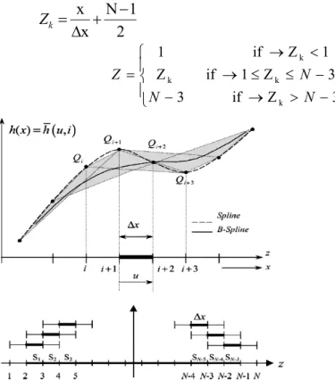
The adaptive spline neural network (ASNN’s) are designed using a neuron, called generalized sigmoid (GS-neuron), containing an adaptive parametric spline activation function. The basic network scheme is therefore very similar to classical multilayer perceptrons (MLP) structures, but with improved nonlinear adaptive activation functions. These functions have several interesting features: (1) easy to adapt, (2) retain the squashing property of the sigmoid, (3) have the necessary smoothing characteristics, (4) easy to implement both in hardware and in software. Spline activation functions are smooth parametric curves, divided in multiple tracts (spans) each controlled by four control points. Let h(x) to be the nonlinear function to reproduce, then the spline activation function can be expressed as a composition of N-3 spans (cubic spline function) where N is the total number of the control points Qj, where j=1,2,……..,N, each is depending on a local variable
[0,1)
u
and controlled by the control points as shown in Fig.2.
y
h(x)
h
(u,
i)
(3.1)where
h
(u,
i)
is the estimated parametric cubic spline function. The parameters can be derived by a dummy variable Z that shifts and normalizes the input.
Z
k2
1
N
x
x
3 Z if 3 3 Z 1 if Z 1 Z if 1 k k k k N N NZ (3.2)
Fig. 2. Locally adaptive B-spline functions, each is defined inside a single span
Where
Δ
x
is the fixed distance between two adjacent control points. The constraints imposed by (3.2) are necessary to keep the input within the active region that encloses the control points. Separating Z into integer and fractional parts using the floor operator
.
will provide,
Z
,
u
Z
-
i
i
(3.3)In the matrix form, the output can be expressed as follows [24]:
y
=
h
(
u
,
i
)
=
Τ
u•
•
Q
(3.4) Where
Τ
=
[
u
3u
2u
1
]
u and
Q
Q
Q
Q
Q
Τ 3 i 2 i 1 i i
i
(3.5) 0 1 4 0 0 3 0 3 0 3 6 3 1 3 3 1 6
1 for
(
B
spline
)
functionor 0 0 2 0 0 1 0 1 1 4 5 2 1 3 3 1 2
1 for
spline
function
Q Q
Q
Q1 2 3 ,... N (3.6)
In each time, only four control points will be involved in the training process. The activation function of the adaptive spline neural network is divided into two parts: GS1 which is used to determine i and u and GS2 which is used to determine Equation (3.4), as shown in Fig. 3.
Fig.3. The spline activation function architecture.
IV.THE PROPOSED SEPARATION METHOD
To solve the problem of the post-nonlinear blind source separation, we need to overcome the distortion of the nonlinear function fin (1.3) and then easy applying a linear blind source separation algorithm. As described in Section 1.2, if the post nonlinear mixed signal is transformed into Gaussian distribution, the nonlinearity of the mixed signal can be eliminated and the problem will be transferred to linear blind source separation problem. A new method for linearization using the principle of the short-time Gaussianization and the B-spline neural network is introduced. This new method has adavantages over the ASNN method in [28] and the Gauss-TD technique in [18]. It is simple in learning rule and simple in separation system. This fact will be proved in the simulation results. The proposed algorithm can be summarized as follows:
Phase A: the Gaussianization steps
(1) Dividing the nonlinear mixed data in the time domain into blocks, for each data vector, and calculate the approximating negentropy Ji(y).
(2) Passing the data block through Gs1 and Gs2 (equation (3.2) to equation (3.5)) as shown in Fig .4. (3) Applying Gaussianization on the output data from Gs2.
(4) Calculate the approximating negentropy Ji+1(y) of the linearized data. Then, check if Ji+1(y) > Ji(y) go to step 1 and change the starting block size else go to the next step.
(5) Updating the control point of the Gs2 (the updating procedure will be described in Section B).
Fig.4. The block diagram of the linearization
Phase B: Multistage QR Factorization (MQRF) Based Rotation steps:
(1) The output data vector Y(t), from part A, will be sphered in the time domain using the whitening matrix W to get a new signals D(t). The whitening matrix will be calculated from the singular value decomposition (SVD) of the cross correlation matrix [25, 26].
(2) Decompose the wide-band whitened signal D(t) into narrow band subcomponents Di(t) using the wavelet packet transform, where i is the wavelet level number.
(3) From the first band in the wavelet domain, the covariance matrix C1will be computed. In this paper, the symbol C will be used to denote the covariance matrix.
(4) Using QR factorization to decompose C1 into unitary matrix Q1 and upper triangular matrix R1 [29].
(5) Multiply the rotating matrix Q1 by the signal in subband 2 then repeat step 3 and step 4 with all subbands to give a set
of unitary matrices as shown in Fig. 5.
(6) Now the rotating matrix Vand the separation matrix can be calculated (estimating the separation matrix is reported in Section A):
(4.1) B=VTW
Q1 D(t) Q2
D2 (k)
.
. QL-1
QL DL (k)
Fig. 5 Block description of QR based rotation matrix estimation
A. Estimating the separation matrix
Assuming that the whitened mixture signals in the wavelet domain is decomposed as follows:
Wavelet Packet Transform
× C2=Q2 R2
×
C1=Q1R1
(4.2) D (k) = D1(k) + D2(k) +….+ DL (k);
Let's assume that the data (covariance) matrix C(D(k)) contain n linearly independent columns C(D1(k)), and let's represent the QR factorization of the data matrix C(D(k))as follows:
(4.3) QTR = C(D(K))
The matrix QT is an orthogonal matrix that takes C(D(K) to upper triangular form. With this insight, it will be good if there is a representation of QT that would enable us to take C(D(K) to upper triangular form, subband by subband. Keeping in mind a representation of QT in factor form as follows:
(4.4) QLT= QL-1 … Q1
where each of the transformations QL is itself orthogonal: QTL QL = I.
If the independent column data matrix of the first subband C(D1(k)) = C1 is constructed from the correlation coefficients of the first corresponding wavelet subbands and is factorized using QR factors; then
(4.5) C1 = Q1R1;
Computing Ψ2(k) which is the rotating component of the second subband (D2(k)) of the whitened mixtures using Q1 and
computing the covariance matrix as follows:
(4.6) Ψ2 (k) = Q1 D2(k) ;
C(Ψ2(k) = Q1 D2(k) D2(k)T Q1T ;
= Q2 R2 .
The third subband will be rotated using Q1 and Q2 such that
(4.7) Ψ3 (k) = Q2 Q1 D3(k);
C(Ψ3(k)) = Q2Q1 D3(k) D3(k)T Q1T Q2T;
= Q3 R3
In general, the factorization of any covariance matrix C(ΨL(k))for any rotated subband L can be written as follows:
(4.8) C(ΨL(k))= QLRL
= QL-1...Q1DL(k) DL (k)T Q1T …QL-1T Also the covariance matrix C(DL(k)) of any whitened subband can be written as follows:
(4.9) C(DL(k)) = Q1T...QL-1T(QL RL) QL-1 ... Q1
Repeat these steps from subband to the next one. When the rotation is converged, RL will be diagonal matrix and Q L will be identity matrix. Then, the separation matrix B can be written as follows:
(4.10) B= QL-1...Q1 W;
while the covariance matrix is rotated as in (4.5), the whitened signals Y(t) can rotate in the time domain by the rotation matrix as follows:
(4.11) VT = Q = QLT QL-1T.… Q1T ;
Note that, the sources may be recovered to within a permutation and a scaling, by matrices § and Є respectively:
P=§ Є = B A (4.12)
PI =
)
1
(
1
n
n
n
i 1
n
j1
1max j ij
ij
P
P
(4.13)
Where [P]ij is the (i,j)-element of the matrix P. The smaller PI implies usually better performance in separation. In the simulation results, the PI value is selected to be 0.005. Sometimes, to achieve this value the wavelet packet decomposition is repeated.
B. The updating process
In the beginning, the data vectors must be normalized to be with zero mean and unit variance. The approximating negentropy is used to measurement the efficiency of the linearization. The term negentropy actually represents negative of entropy. The negentropy J(y) of the random variable y is given by
H(Y)
)
H(Y
J(Y)
gauss
(4.14)where H(.) is the differential entropy of (.) and Ygauss is the Gaussian random variable with the same covariance as of Y. This definition of negentropy ensures that it will be zero if Y is Gaussian and will be increasing if Y is becoming non-Gaussian. This implies that it is always positive. Thus negentropy based contrast function can be minimized to obtain optimally Gaussian component. However, estimation of true negentropy, as in (4.14), is difficult and it requires knowledge of probability distribution function of the data. Thus several approximations for negentropy estimation have been used and proposed. Some of this approximation has been based on the generalized Higher Order Statistics (HOS) which uses some nonlinear non-quadratic functions G. In terms of such function the most widely used approximation of negentropy is given by [31, 32]
2 gauss
)]
(G(Y
E
[E(G(Y))
J(Y)
(4.15)where
is a positive constant and Ygauss is a Gaussian random variable with the same covariance as that of Y. The optimally Gaussian component can be obtained by minimizing (4.15). The performance of the optimization algorithm depends on the used non-quadratic nonlinear function G. It is desirable that the function G should provide robustness toward outlier values in the data and should provide better approximation to true negentropy. Better robustness to outliers can be ensured by choosing G with slow variation with respect to change in data and, at the same time, very close approximation of negentropy can be expected if statistical characteristics of G inherits PDF of the data. Choosing G(y) = log (Cosh(y)) gives G'(y) = tanh(y) and G``(y) = 1 - tanh 2(y). The tanh function is the most suitable to use among all non-quadratic functions and provides the best results even for both super- and sub-Gaussian sources [31].To drive the equation which controlling the updating of the control point vector Q, the derivative of the equation (4.15) with respect to the control points vector Q must be calculated. Since the vector, Y is a function of the control point vector Q. So
Q Y J
will equal to:
2 gauss
)]
(G(Y
E
[E(G(Y))
Q
λ
=
Q
J(Y)
(4.16) Since Ygauss is a Gaussian random variable with the same covariance as that of Y so2 m Y
e
2
1
gauss
Y
, whereσ
=
E[(y
-
m)
2]
(4.17) The assumption of the data vectors to be normalized with zero mean and unit variance will provide the Ygauss equation is:y
e
2
1
So
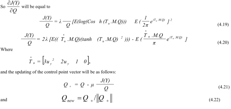
Q
J(Y)
will be equal to
2 .M.Q) (T
u 2π e ]
1 ( E .M.Q))) (T h [E(log(Cos Q Q J(Y) u = (4.19)
π
e
]
.M.Q
T
(
E
-)))
.M.Q)
(T
.M.Q)(tanh
T
[E((
2
=
Q
J(Y)
u (T .M.Q)• 2 u • u u (4.20) Where
Τ
u=
[
3
u
y22
u
y1
0
]
•
,
and the updating of the control point vector will be as follows:
Q
J(Y)
Q
Q
+=
-
(4.21)and
Q
new
Q
/
Q
(4.22) The learning rate of the algorithmμ
was tuned to 0.002 in our simulations. The expectation “E” operator can be dropped in the updating of the control points in Equation (4.20) but it cannot be dropped in the negentropy Equation (4.16).V. SIMULATION RESULTS AND IMPLEMENTATION
In this section, several types of signals are used to evaluate the performance of the proposed technique. In the following experiments
Δ
x
is selected to be 0.2 and the initial value of the control points is selected from sampling the sigmoid function ( x x e 1 e 1 ).In the QR factorization step, maximum 3-stage of the wavelet packet transform is used to get 5-subband components. In the proposed algorithm, there are some assumptions are considered as follows: (1) the source signals must be independent, (2) the number of mixed signals are greater than or equal to the number of the source signals, (3) there is at most one source signal have Gaussian distribution, (4) the nonlinear function f is invertible function, and (5) the mixed matrix must be of full rank.
Experiment 1: The proposed algorithm is applied on audio signal with length of 32000 samples mixed with Gaussian noise
(0,5)
using nonlinear mixture in (5.1) and (5.2). The scattering plot of the original signals, the mixed signals and the estimating signals are shown in Fig 6. The proposed algorithm can give a clear separation of the nonlinear mixing signals. Fig. 7 shows, respectively, the original signals, the nonlinear mixture X(t) and the separated signals for this exampleAS(t)
Z(t)
(5.1)Where
.92
.3
.2
.8
A
and (t)) 2 (3Z (t)) 2 (Z (t) X (t)) 1 .3Z (t)) 1 (Z (t) Xsin
cos
e
2 1 (5.2)
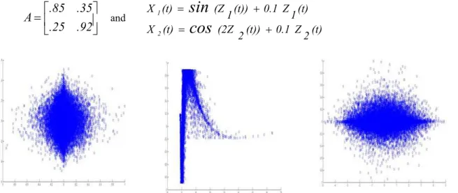
.92
.25
.35
.85
A
and(t) 2 Z 0.1 (t)) 2 (2Z (t)
X
(t) 1 Z 0.1 (t)) 1 (Z (t)
X
cos
sin
2 1
(5.3)
(a) (b) ( c)
Fig.6. Experiment 1:(a) scatter plot of the original data. (b) Scatter plot of the mixed data. (c) scatter plot of the estimated data
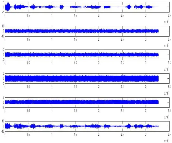
Fig. 8. Experiment 2: the original data are the first two signals on the top, the mixing data are in the middle and the recovering data are in the last two rows.
(a) (b)
Fig.9. Experiment 2:(a) scatter plot of the mixed data. (b) scatter plot of the estimated data
Experiment 3: The proposed algorithm is applied on two audio signals with length of 30000 samples using the following mixing system (proposed in [27]). Fig. 10 shows, respectively, the original signals, the nonlinear mixture X(t) and the separated signals for this example. Moreover, the scattering plot of the original signals, the mixed signals and the estimating signals are shown in Fig 11. We see that, almost perfect reconstruction of the original signals is achieved. The mixed model uses a random matrix A and nonlinear function Where
(t))
2
tanh(10Z
(t)
2
X
3
(t))
1
(Z
(t)
1
X
Fig. 10. Experiment 3: the original data are the first two signals on the top, the mixing data are in the middle and the recovering data is in the last two rows.
(a) (b) ( c)
Fig.11. Experiment 3: (a) scatter plot of the original data. (b) Scatter plot of the mixed data. (c) scatter plot of the estimated data
Experiment 4: Consider a two-channel nonlinear mixture with cubic nonlinearity: this model is introduced in [28].
2 1 3
3
2 1
(.)
(.)
s
s
A
B
x
x
Where the matrices B and A are defined as follows:
.5
.9
-.9
.5
A
.25
.86
.86
.25
B
)
t
20
sin(
)
t
(
S
π
t)
100
(
cos
π
t))
6
(
sin
5
.
0
(
(t)
S
2 1
Fig. 12 shows, respectively, the original signals, the nonlinear mixture X(t) and the separated signals for this example.
Fig. 12 the original data are the first two signals on the top, the mixing data are in the middle and the recovering data are in the last two rows.
This example is used to compare the performance of the proposed technique with the Gauss-TD separation algorithm in [18] and the adaptive spline neural network (ASNN) separation algorithm in [28]. Fig.13 shows, respectively, the original signals, the nonlinear mixture X(t) and the separated signals when applying the Gauss-TD method on the post-nonlinear mixed signal in Example 4. The result of applying the ASNN algorithm on the same signal is introduced in [28].
Fig. 13 Experiment 4: The output result after using the Gauss-TD algorithm in separation
VI. CONCLUDING REMARKS
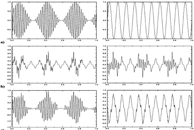
Fig. 14 Experiment 4: the output results from ASNN algorithm (a) two source signals: a modulated signal and a sinusoid. (b) Nonlinear mixtures of source signals. (c) Separated signals.
References
[1] Amari, A. Cichocki, and H. H. Yang, A new learning algorithm for blind signal separation. In NIPS 95, MIT Press, (1996) 882–893.
[2] Bell and T. Sejnowski, information-maximization approach to blind separation and blind deconvolution, Neural Computation, 7 (1995)
1129–1159.
[3] Cardoso, Infomax and maximum likelihood for source separation, IEEE Letters on Signal Processing, 4(1997) 112–114.
[4] W. Lee, M. Girolami, and T. Sejnowski. ,Independent component analysis using an extended infomax algorithm for mixed sub-gaussian and
super-gaussian sources, Neural Computation, 11(1999) 417–441.
[5] D. T. Pham and J.-F. Cardoso, Blind separation of instantaneous mixtures of non-stationary sources, IEEE Trans. on Signal Processing, 49(9)
(2001) 1837-1848.
[6] C. Jutten and A. Taleb, Source separation: from dusk till dawn, in Proc. 2nd Int. Workshop on Independent Component Analysis and Blind
Source Separation (ICA2000), Helsinki, Finland, (2000) 15–26..
[7] A. Hyvarinen and P. Pajunen, Nonlinear independent component analysis: Existence and uniqueness results, Neural Networks, 12(3) (1999)
429–439.
[8] A. Taleb and C. Jutten, Source separation in post-nonlinear mixtures, IEEE Trans. on Signal Processing, 47(10) (1999) 2807–2820.
[9] A. Taleb, A generic framework for blind source separation in structured nonlinear models,” IEEE Trans. on Signal Processing, 50(8) (2002)
1819–1830.
[10] J. Eriksson and V. Koivunen, Blind identifiability of class of nonlinear instantaneous ICA models, in Proc. of the XI European Signal Proc.
Conf. (EUSIPCO 2002), Toulouse, France, 2 (2002) 7–10.
[11] Luis B. Almeida, Linear and nonlinear ICA based on mutual information, the MISEP method, Signal Processing, Special Issue on
Independent Component Analysis and Beyond 84(2) (2004) 231–245.
[12] Tobias Blaschke and Laurenz Wiskott . Independent Slow Feature Analysis and Nonlinear Blind Source Separation .Proc. of the 5th Intl.
Conf. on Independent Component Analysis and Blind Signal Separation Granada, Spain, September (2004) 22-28
[13] S. Squartini, A. Bastari and F. Piazza, "A practical Approach on Gaussianization for post-Nonlinear under-determined BSS,” in the proc. of
the 4th international symposium on neural networks, China (2007).
[14] Taleb and C. Jutten. Nonlinear source separation: The post-nonlinear mixtures. In Proc. European Symposium on Artificial Neural Networks,
Bruges, Belgium, (1997)279–284.
[15] T. W. Lee, B.U. Koehler, and R. Orglmeister. Blind source separation of nonlinear mixing models. IEEE International Workshop on Neural
Networks for Signal Processing,(1997) 406–415.
[16] H.H.Yang, S. Amari, and A. Cichocki. Information-theoretic approach to blind separation of sources in non-linear mixture. Signal Proc.,
64(3)(1998)291–300,
[17] D. Erdogmus, R. Jenssen, Y. N. Rao, J. C. Principe, "Gaussianization: an efficient multivariate Density estimation technique for statistical
signal processing," Journal of VLSI Signal Processing, 45(2006) 67–83.
[18] A. Ziehe, M. Kawanabe, S. Harmeling, and K.-R. M¨uller. Separation of post-nonlinear mixtures using ACE and temporal decorrelation.
[19] C. Jutten and J. Karhunen. Advances in nonlinear blind source separation. In Proc. of the 4th Int. Symp. on Independent Component Analysis and Blind Signal Separation (ICA2003), Nara, Japan, Invited paper in the special session on nonlinear ICA and BSS, April (2003)245–256.
[20] L.E. Larson. Radio frequency integrated circuit technology low-power wireless communications. IEEE Personal Communications,
5(3)(1998)11–19.
[21] A. Ziehe, K.-R. M¨uller, G. Nolte, B.-M. Mackert, and G. Curio. Artifact reduction in magnetoneurography based on time-delayed
second-order correlations. IEEE Trans. Biomed. Eng., 47(1)(2000)75–87.
[22] H. Kantz and T. Schreiber. Nonlinear time series analysis. Cambridge University Press, Cambridge,UK, (1997).
[23] Y Yanlu Xie, Beiqian Dai and Jun Sun, Kurtosis Normalization after Short-Time Gaussianization for Robust Speaker Verification,
Proceedings of the 6th World Congress on Intelligent Control and Automation, Dalian, China June (2006) 21 – 23.
[24] Stefano Guarnieri, Francesco Piazza, Multilayer Feedforward Networks with Adaptive Spline Activation Function, IEEE Transactions On
Neural Networks, 10( 3) May (1999).
[25] A. Belouchrani, K. Abed-Meraim, J. Cardoso, and E. Moulines, "A blind source separation technique using second-order statistics", IEEE
Trans. Signal Processing, 45 (1997) 434 - 444.
[26] J. Cardoso, and A. Souloumiac, "Blind Beamforming for non-Gaussian signals", Proc. IEE- F, 140(6) (1993)362-370.
[27] TeTe-Won Lee, Jean-Franc¸ois Cardoso, Erkki Oja and Shun-Ichi Amari. Blind Separation of Post-nonlinear Mixtures using Linearizing
Transformations and Temporal Decorrelation. Journal of Machine Learning Research 4 (2003) 1319-1338.
[28] MiMirko Solazzi and Aurelio Uncini, "Spline Neural Networks for Blind Separation of Post-Nonlinear-Linear Mixtures" IEEE transactions
on circuits and systems—i: regular papers, 51(4)(2004) 817-829.
[29] Louis L. Scharf, statistical signal processing: detection, estimation, and time series analysis, Reading, Massachusetts, Addison-Wesley
publishing company (1991).
[30] A. Cichocki and S.-I. Amari, "Adaptive Blind Signal and Image Processing: Learning Algorithms and Applications," John Wiley & Sons,
(2002).
[31] A. Hypavarinen, J. Karhunen, and E. Oja. Independent Component Analysis. JohnWiley & Sons, (2001).
[32] Elsabrouty, M. Bouchard, M. Aboulnasr, T., “A new on-line negentropy-based algorithm for blind source separation” IEEE International