www.ann-geophys.net/34/1109/2016/ doi:10.5194/angeo-34-1109-2016
© Author(s) 2016. CC Attribution 3.0 License.
Spatial and temporal variation of total electron content as revealed
by principal component analysis
Elsayed R. Talaat1,aand Xun Zhu1
1The Johns Hopkins University Applied Physics Laboratory, 11100 Johns Hopkins Road, Laurel, MD 20723, USA anow at: Heliophysics Division, NASA Headquarters, Washington, D.C. 20546, USA
Correspondence to:Xun Zhu ([email protected])
Received: 14 July 2016 – Revised: 30 September 2016 – Accepted: 6 November 2016 – Published: 29 November 2016
Abstract.Eleven years of global total electron content (TEC) data derived from the assimilated thermosphere–ionosphere electrodynamics general circulation model are analyzed us-ing empirical orthogonal function (EOF) decomposition and the corresponding principal component analysis (PCA) tech-nique. For the daily averaged TEC field, the first EOF ex-plains more than 89 % and the first four EOFs explain more than 98 % of the total variance of the TEC field, indicating an effective data compression and clear separation of different physical processes. The effectiveness of the PCA technique for TEC is nearly insensitive to the horizontal resolution and the length of the data records. When the PCA is applied to global TEC including local-time variations, the rich spatial and temporal variations of field can be represented by the first three EOFs that explain 88 % of the total variance. The spectral analysis of the time series of the EOF coefficients re-veals how different mechanisms such as solar flux variation, change in the orbital declination, nonlinear mode coupling and geomagnetic activity are separated and expressed in dif-ferent EOFs. This work demonstrates the usefulness of using the PCA technique to assimilate and monitor the global TEC field.
Keywords. Ionosphere (ionospheric disturbances)
1 Introduction
The ionosphere is highly variable and has a complex system of drivers including variable solar radiation plus geomagnetic activity from the upper atmosphere and momentum and en-ergy fluxes associated with neutral wind dynamics from the lower atmosphere. While magnetospheric forcing dominates the variability at high latitudes in the ionosphere,
photochem-istry and neutral dynamics play dominant roles in the iono-spheric structure and variability at mid- and low latitudes. One critical quantity describing the ionosphere and its vari-ability is the total electron content (TEC). A variety of in situ and remote-sensing techniques has been employed to study the Earth’s ionosphere in terms of the electron density. The method and platform used for measurement determine reso-lution in time and space, with the measurement often being distributed unevenly. Unless assimilated general circulation models are used, no one method effectively allows for the sampling of large areas of the ionosphere with high and uni-form resolution in both time and space. Since ionospheric electronic densities respond to a complex set of highly vari-able driving mechanisms, the global characterization of the response to solar variability posts a significant challenge.
1110 E. R. Talaat and X. Zhu: Spatial and temporal variation of total electron content
space induced by different kinds of physical processes are the main characteristics of the ionosphere.
In this paper, we perform a set of multi-year assimilated runs of the thermosphere–ionosphere electrodynamics gen-eral circulation model (TIEGCM) (Roble et al., 1988; Rich-mond et al., 1992) driven by a lower boundary condition of tidal forcing derived from the Sounding of the Atmosphere using Broadband Emission Radiometry (SABER) instrument (Talaat and Lieberman, 1999; Talaat et al., 2001). To effec-tively decompose and understand the complicated temporal and spatial variations of the ionosphere, we apply the empir-ical orthogonal function (EOF) and the associated principal component analysis (PCA) to the TEC fields derived from the TIEGCM runs. Section 2 describes the EOF and PCA nota-tions and their application to different TEC fields. Section 3 shows how the EOF and PCA are able to reveal major phys-ical processes associated with different EOFs derived from data fields. Section 4 provides a final summary and conclu-sions.
2 EOF and PCA of the assimilated TEC
2.1 A brief review and notations of the EOF and PCA The empirical orthogonal function (EOF) and the corre-sponding principal component analysis (PCA) are the stan-dard statistical techniques for analyzing atmospheric data since being introduced by E. N. Lorenz in 1956 (Wilks, 2006). The PCA technique decomposes a given spatial– temporal field such as TEC into a set of base functions called EOFs that is internally determined from the data sets. Letun=un,ij =u(tn;xi, yj)denote the time series of
the measured or the assimilated TEC field at N time steps overK=I×J spatial grids (n=1,2, . . ., N;i=1,2, . . ., I; j =1,2, . . ., J ), where tn, xi and yj denote time,
longi-tude and latilongi-tude, respectively. Then, the PCA expresses the spatial–temporal fieldunby its time-averaged fieldu¯(=
N−16nN=1un)and a set of EOFs (vm,m=1,2, . . ., K)that
do not vary with time (Preisendorfer, 1988, Wilks, 2006):
un= ¯u+u′n= ¯u+ K
X
m=1
Em,nvm, n=1,2, . . ., N, (1)
where the principal component (PC)Em,nis the time series
of the decomposition coefficient that characterizes the tem-poral variation of the original fieldun being projected onto
themth EOFvm. Furthermore, different PCs are orthogonal
to each other in time (Preisendorfer, 1988).
Equation (1) is a reconstruction formula and can be con-sidered as a linear transform that projects the original pertur-bation fieldun− ¯uonto a set of base functions{vm}. Since
EOFs are derived from the data rather than prescribed base functions such as spherical harmonic functions that are often used for analyzing global data, the most information on the
original field that represents the physics and its variations can be expressed by a highly truncated Eq. (1) withM≪K,
un≈ ¯u+ M
X
m=1
En,mvm, n=1,2, . . ., N. (2)
The effectiveness of the PCA can be quantitatively measured by the ratio of the percentage of the total variance inun− ¯u
explained by individual EOFs: rm2= Var(Em,nvm)
Var(un− ¯u)
×100 %. (3)
The value ofrm2 is proportional to the magnitude of themth eigenvalue (λm)of the covariance matrix ofun− ¯uthat
de-creases withm(Wilks, 2006). Since different EOFs are or-thogonal to each other in space, the explained variance by the truncated PCA expression Eq. (2) for differentMis given by
RM2 =
M
X
m=1
rm2. (4)
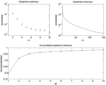
Figure 1.Explained variancerm2vs.mand the accumulated explained varianceR2Mvs.Mfor the daily averaged global TEC over an 11-year time period (4180 days) from 1999 to 2010 and 72×71 spatial grids.
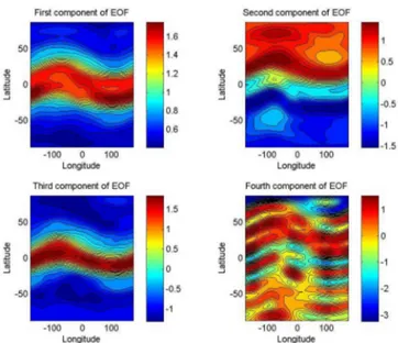
Figure 2.First four EOFs for the 11-year daily averaged global TEC as functions of longitude and geographic latitude calculated by the spatial and temporal settings given in Fig. 1.
in the latitudinal direction that is mainly also caused by the solar radiation and cannot be fully represented by the first EOF. The fourth EOF (withr42=0.5 %) shows much smaller wave structure in both longitudinal and latitudinal directions. Since the EOFs are determined internally from the data, it is worthwhile examining in this application how sensitive the derivedR2M and EOFs are with respect to the data we used. Figures 3 and 4 show the same calculations as in Figs. 1 and 2
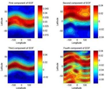
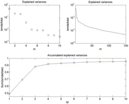
for a 6-year period with 2190 days from 1999 to 2004. Com-parison between the two sets of figures shows that the change in the length of the spatial–temporal field only slightly mod-ifies PCA output. Though the record of the data has been cut shorter by about one half, the first EOF still explains 79.4 % and the combination of the first four EOFs explains 96.4 % of the total TEC variance. More importantly, the spatial pat-terns of the first four EOFs, shown in Fig. 4, are also very similar to those shown in Fig. 2.
fea-1112 E. R. Talaat and X. Zhu: Spatial and temporal variation of total electron content
Figure 3.Same as Fig. 1 except for a 6-year time period (2190 days) from 1999 to 2004.
Figure 4.Same as Fig. 2 except for a 6-year time period (2190 days) from 1999 to 2004.
tures cannot be fully resolved by a lower-resolution analysis (r42=0.4 % in Fig. 1 vs.r42=0.5 % in Fig. 5).
2.3 EOF and PCA applied to hourly TEC
Next, we examine the TEC field that includes the local-time variations. The PCA is applied to theu(tn;xi, yj)field with
the lower-resolution spatial grid of Figs. 5 and 6 but with a temporal resolution of 2 h. The total number of time steps N =50 160, which corresponds to 11.4 years of time interval starting from 1999. Figures 7 and 8 show plots of(rm2, RM2)
and the first six EOFs. We first note that (Fig. 7) the contribu-tion by the first EOF (48.8 %) is significantly lower than one shown in the daily averaged TEC analysis (Figs. 1, 3 and 5), indicating a weaker correlation or a richer structure in spatial and temporal variability of the TEC field. This is expected since unlike the daily averaged field, the local-time tion introduces additional and stronger longitudinal varia-tions due to the local-time response of TEC that is directly related to the solar radiation forcing. The sum of the first six EOFs makes up approximately 93.6 % of the total vari-ance. Another significant feature shown in Fig. 7 is that the second and third EOFs contribute almost equally (20.4 and 18.6 %) to the total variance. The spatial pattern of the first EOF in Fig. 8 is almost identical to that shown in Fig. 2, mainly representing the effects of daily averaged solar forc-ing and the dominant wave number 1 feature due to the off-setting geomagnetic field. The next two EOFs shown in Fig. 8 represent longitudinal variation of wave number 1 with ap-proximately equal magnitudes and π/2 phase shift. These two natural modes represent the major contributions from the first two components of the sinusoidal decomposition in lon-gitude sin(π xi/180)and cos(π xi/180)caused by the
Figure 5.Same as Fig. 1 except for a spatial resolution of 36×35 grids.
Figure 6.Same as Fig. 2 except for a spatial resolution of 36×35 grids.
One expects that the paired EOFs(v6,v7)and(v8,v9)
rep-resent the high harmonics of the longitudinal variance asso-ciated with the local-time variation of the solar forcing. We have also performed sensitivity analyses for the case simi-lar to Figs. 3 and 4 by applying PCA to shorter data records of 4 years that correspond to either solar maximum (1999– 2003) or solar minimum (2006–2009). In terms of their spa-tial structure, the derived EOFs are almost identical to those shown in Fig. 8.
3 Physical processes as objectively revealed by EOFs and TEC
One major advantage of the PCA technique is the data com-pression, so the physical field is effectively projected onto a few modes that include the majority of the variance of the original field. We have already shown that the four EOFs in Fig. 2 and the six EOFs in Fig. 8 contain 98.2 and 93.6 % of the total variance, respectively. Based on their spatial pat-terns, we have also indicated in the above analysis that there exist clear physical mechanisms that drive the different EOFs solely derived from the data. To illustrate the roles played by different physical mechanisms in extracting EOFs, we show in Fig. 9 the time series of the decomposition coefficients Em,n, i.e., PCs, of the PCA for the first four EOFs, shown in
Fig. 2. The specific physical mechanisms are best described in byE1,nandE2,n. Sincev1andv2in Fig. 2 mainly
repre-sent the effects of the solar radiation and the seasonal varia-tion of the inclinavaria-tion angle of the Earth’s orbit, the two time series plotted in the upper panel of Fig. 9 show the responses of the 11-year solar cycle and annual oscillation. Note that the variance contributed fromv3andv4is far less than those
from v1 andv2 (Fig. 1). This is also reflected by the fact
that the magnitudes ofE3,nandE4,nare much smaller than
those ofE1,n andE2,n. Furthermore, since neither effect of
the solar radiation nor the seasonal variation is orthogonal in space, the remaining EOFs, includingv3andv3together with
their coefficientsEm,n, will include both effects, as indicated
above and also shown in the lower panel of Fig. 9.
1114 E. R. Talaat and X. Zhu: Spatial and temporal variation of total electron content
Figure 7.Explained variancerm2 vs.mand the accumulated explained varianceR2Mvs.Mfor the global TEC over an 11-year time period (4180 days) from 1999 to 2010 with a 2 h temporal resolution and 36×35 spatial grids.
Figure 8.First six EOFs for the 11-year global TEC as functions of longitude and geographic latitude calculated by the spatial and temporal settings given in Fig. 7.
TECU (1 TECU=1016electrons m−2) at five different lati-tudes: Equator (0◦), 37.5◦S, 37.5◦N, 62.5◦S and 62.5◦N. Also shown in the figure is the dailyF10.7that is the 10.7 cm solar radio flux (in units of 10−22W m−2Hz−1) and that measures the intensity of the solar activity. The overall cor-relation betweenF10.7 and TEC is overwhelming, suggest-ing that the solar radiation and/or solar wind are the ultimate
be-Figure 9.Time series of the principal components of the PCA for the first four EOFs shown in Fig. 2:E1,n, E2,n– blue, green lines in panel(a);E3,n, E4,n– blue, green lines in panel(b).
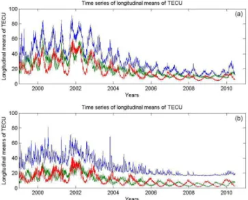
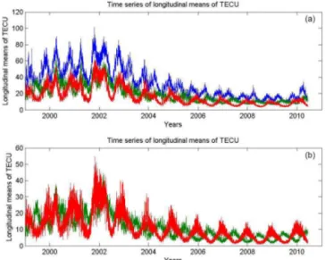
Figure 10. Daily mean time series of the longitudinally aver-aged TEC at five different latitudes: 0◦, 37.5◦S, 37.5◦N – blue, green, red lines in panel(a); 62.5◦S, 62.5◦N – green, red lines in panel (b). The blue line in panel(b) denotesF10.7, which is the 10.7 cm solar radio flux (in units of 10−22W m−2Hz−1).
tween the southern latitude and northern latitude time series. In other words, the five time series of TEC shown in Fig. 10 are highly correlated so that the information in Fig. 10 con-tains a significant redundancy. Note that the time series of Em,ncoupled with the basis function{vm}in the highly
trun-cated expansion Eq. (2) represent the entire spatial–temporal field. In Fig. 11, we show the differences of the TEC time se-ries shown in Fig. 10 and the ones calculated based on Eq. (2) withM=4. Comparison between Figs. 10 and 11 shows that differences are small and close to irregular, suggesting that
Figure 11.Differences in TEC time series between those shown in Fig. 10 and the ones calculated based on highly truncated expansion Eq. (2) withM=4 at five different latitudes: 0◦, 37.5◦S, 37.5◦N – blue, green, red lines in panel(a); 62.5◦S, 62.5◦N – green, red lines in panel(b).
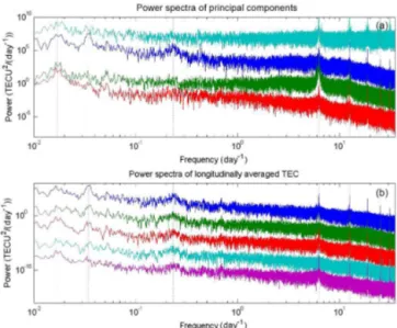
Figure 12.Fourier power spectra of the first four PCs shown in Fig. 9 (panela) and the time series at five different latitudes shown in Fig. 10 (panelb). To avoid clustering, all the curves except the first PC in the upper panel and the one at the Equator in panel(b)
have been consecutively shifted downward by 3 orders of magni-tude.
the first four EOFs together with the four PCs have included major physical processes that control the TEC distribution and variations.
1116 E. R. Talaat and X. Zhu: Spatial and temporal variation of total electron content
Figure 13.Time series of the principal components of the PCA for the first EOFs shown in Fig. 8:Eamp, E1,n, E4,n– blue, green, red
lines.
Figure 14.Scatterplots between the daily averagedF10.7and the daily averaged time series (Eamp, E1,n, E4,n) shown in Fig. 13: (Eamp, E1,n, E4,n)– (blue, green, red) dots.
more clearly and quantitatively shown in the figure that the major spectral features among different EOFs are different, whereas those among the longitudinally averaged TEC at dif-ferent latitudes are nearly the same. The first EOF spectrum peaks at all four frequencies, whereas the second EOF only shows one striking peak in the annual period that is domi-nant over the entire spectral domain. For the third and fourth EOFs, only two peaks at semiannual and 27-day periods are noticeable. Since different spectral characters often corre-spond to different driving mechanisms, Fig. 12 suggests that the PCA technique is able to differentiate directly between physical mechanisms and the data.
Figure 15.Two-hour resolution time series of the longitudinally averaged TEC at five different latitudes: 0◦, 40◦S, 40◦N – blue, green, red lines in panel (a); 60◦S, 60◦N – green, red lines in panel(b).
Figure 13 shows the time series of PCA for the case of Fig. 8, which includes local-time variationEamp,E1,n and
E4,n, whereEampis the amplitude of the time series for the paired EOFs(v2,v3):
Eamp=
q
E2,n2+ E3,n2,
Ephase=tan−1 E3,n/E2,n
. (5)
Note that the paired EOFs(v2,v3)shown in Fig. 8 denote
the fixed spatial patterns of the local-time variations with a π/2 phase shift. As a result, the corresponding paired coef-ficients(E2,n, E3,n)are expected to have similar magnitudes
and change rapidly with the local time in order to represent a moving wave structure. The amplitude defined in Eq. (5) combines the effects of both components and also eliminates the local-time variation. We also note from Fig. 13 thatE1,n
andEamp are highly correlated with a dominant period of about half a year thoughE1,n is not correlated with either
E2,nor E3,n. This is because the first three EOFs all
repre-sent the effect of solar radiation. On the other hand, the fourth EOF shows a clear signature of annual cycle that corresponds to the effect of the inclination angle of the Earth’s orbit. Such a difference in the effects of solar radiation on the differ-ent EOF compondiffer-ents can also be seen from Fig. 14, which shows the scatterplots between the daily averagedF10.7and the daily averaged time series(Eamp, E1,n, E4,n)shown in
Fig. 13. The figure shows thatF10.7is well correlated with both E1,n and Eamp, whereas E4,n appears to be
sug-Figure 16. Fourier power spectra of the first four PCs shown in Fig. 13 (panela) and the time series at five different latitudes shown in Fig. 14 (panelb). To avoid clustering, the green and red curves in(a)have been moved down by 3 and 6 orders of magnitude, re-spectively. All the curves except the one at the Equator in(b)have been consecutively shifted downward by 3 orders of magnitude. The cyan curve in paneladenotes the spectrum of the phase 104Ephase defined in Eq. (5).
gesting that the longitudinal and local-time averages are not interchangeable for the TEC field.
In Fig. 16, we show the Fourier power spectra for the time series shown in Figs. 13 and 15. The six vertical lines denote the peak frequencies that correspond to the following peri-ods: annual, semiannual, 27-day, 1-day, 0.5-day and 0.25-day. Panel a in the figure shows that Eamp has significant spectral peaks in all the noted frequencies, whereas Ephase does not show spectral peaks at the 27-day and semiannual periods. We also note that there are significant sub-harmonic peaks in the Eamp spectrum for a frequency greater than 2π/1-day. The spectral peaks at 3π/1-day and 5π/1-day re-sult from the sum of spectral peaks at 2π/1-day plusπ/1-day and 3π/1-day plus 2π/1-day, respectively. Again, the spectral features ofEampare similar to that for the third EOF shown in Fig. 13, whereas the spectrum for the fourth EOF is dom-inated by the annual cycle, also consistent with the results shown in Fig. 13.
4 Summary and conclusions
In this study, we apply the EOF and PCA to the global TEC data derived from TIEGCM forced under the realistic solar inputs from above the SABER-observed tidal waves from be-low. We demonstrate the effectiveness of the EOF decompo-sition of the ionospheric variations in both time and space. It is shown that for the daily averaged TEC field, the first EOF explains more than 89 % and the first four EOFs
ex-plain more than 98 % of the total variance of the TEC field. When PCA is coupled with the spectral analysis of the time series of the EOF coefficients, it is also shown that the EOF analysis is not only a data compression technique but also a powerful tool to objectively reveal the relative importance of individual physical mechanisms (such as solar flux variation, change in the orbital declination, nonlinear mode coupling and geomagnetic activity) that are responsible for the total TEC variance.
5 Data availability
The TIEGCM output TEC fields that generated all the figures in this paper are available from Xun Zhu ([email protected]) upon request.
Acknowledgements. This research was supported by NASA Liv-ing With a Star Program under grants NNX09AJ61G and NNX13AF91G and the Heliophysics Supporting Research program under grant NNX16AG68G to the Johns Hopkins University Ap-plied Physics Laboratory. Comments on the paper by two anony-mous reviewers are greatly appreciated.
The topical editor, K. Shiokawa, thanks two anonymous referees for help in evaluating this paper.
References
Lean, J.: Solar ultraviolet irradiance variations: A review, J. Geo-phys. Res., 92, 839–868, 1987.
Preisendorfer, R. W.: Principal Component Analysis in Meteorol-ogy and Oceanography, edited by: Mobley, C. D., Elsevier, Am-sterdam, the Netherlands, 425 pp., 1988.
Richmond, A. D., Ridley, E. C., and Roble, R. G.: A thermo-sphere/ionosphere general circulation model with coupled elec-trodynamics, Geophys. Res. Lett., 19, 601–604, 1992.
Roble, R. G., Ridley, E. C., and Richmond, A. D.: A coupled ther-mosphere/ionosphere general circulation model, Geophys. Res. Lett., 15, 1325–1328, 1988.
Talaat, E. R. and Lieberman, R. S.: Nonmigrating diurnal tides in the mesosphere and lower thermosphere, J. Atmos. Sci., 56, 4073–4087, 1999.
Talaat, E. R., Yee, J.-H., and Zhu, X.: Observations of the 6.5-day wave in the mesosphere and lower thermosphere, J. Geophys. Res., 106, 20715–20724, doi:10.1029/2001JD900227, 2001. Tobiska, W. K.: Recent solar extreme ultraviolet irradiance
obser-vations and modeling: A review, J. Geophys. Res., 98, 18879– 18893, 1993.