Numerical analysis of CFRP mesoscale models

(1)

Setembro 2016

Pedro Miguel Ferreira de Sousa Pepe Mangualde

Licenciado em Ciências da Engenharia Mecânica

Numerical analysis of CFRP

mesoscale models

Dissertação para obtenção do Grau de Mestre em

Engenharia Mecânica

Orientador: Professor Doutor João Mário Burguete Botelho Cardoso, Professor

Auxiliar da Faculdade de Ciências e Tecnologias da Universidade Nova

de Lisboa

Co-Orientador: Doutor Pedro Miguel de Almeida Talaia, Engenheiro de I&D, CEiiA

Júri:

Presidente: Doutor Pedro Samuel Gonçalves Coelho Vogais: Doutor Bernardo Rodrigues de Sousa Ribeiro

Doutor Pedro Miguel de Almeida Talaia

(2)

(3)

i

Copyright

(4)

(5)

(6)

(7)

v

Acknowledgment

I would first like to thank my dissertation advisor Auxiliary Professor Doctor João Mário Burguete Botelho Cardoso of the Faculdade de Ciências e Tecnologia at

Universidade Nova de Lisboa, for his guidance, advices, help and patient provided

throughout the dissertation and my academic career.

I would also like to thank all professors of the Faculdade de Ciências e Tecnologia at Universidade Nova de Lisboa from the several departments but especially to the all professors of the Mechanical and Industrial Engineering department. They were fundamental to my graduation and contributed to the success of my academic career.

I would also like to acknowledge Faculdade de Ciências e Tecnologia at Universidade Nova de Lisboa for providing the facilities and equipment fundamental to this dissertation.

I would like to thank CEiiA and Doctor Pedro Miguel de Almeida Talaia, my co-supervisor, for the opportunity to work on this dissertation and learn with them.

I would also like to thank my course and laboratory colleagues, who accompanied me throughout my academic life, helping me throughout the course and providing a friendly and cheerful work environment.

(8)

(9)

vii

Abstract

Composite materials, specifically Carbon Fiber Reinforced Polymers, have a complex mechanical behaviour, therefore it is extremely complicated to predict failure and damage.

There has been an increasing use of composite materials for structural applications as an alternative to metal due its lightweight and strength properties. Consequently, it is important to consolidate the knowledge about its behaviour under different loads in order to apply them correctly in structural applications.

The Carbon Fiber Reinforced Polymer studied in this dissertation is a spread tow carbon fabric with four different arrangements - 0°/-90°, 15°/-75°, 30°/-60° and 45°/-45° under tension loads.

A computational tool was developed in order to predict failure and damage propagation in Carbon Fiber Reinforced Polymers specimens. It is an interface program between the software Matlab and ANSYS. A mesh generator algorithm was developed in Matlab in order to automatically model specimens with different arrangements. Afterwards, an incremental iterative analysis is performed using an optimized methodology developed in _Crespo’s dissertation [3] which gradually increments the displacement applied to the specimen. This analysis uses ANSYS as a solver, using the finite element method, to calculate the _{specimen’s m}echanical behaviour and stress. The results are exported to Matlab, which applies a proposed failure criterion to the specimen’s elements and initiates ANSYS “killing” the failed elements and applying a new displacement. The program executes several iterations until the specimen’s failure and, in the end, plots the force applied and displacement in the specimen’s end.

The numerical models were validated with numerous analysis using experimental and numerical results from articles and dissertations from different authors in order to guarantee the precision of the results and simulations.

(10)

(11)

ix

Resumo

Materiais compósitos, mais especificamente fibra de carbono, têm um comportamento mecânico complexo, o que torna extremamente complicado para prever falha e dano.

Existe um uso crescente de material compósito para aplicações estruturais como alternativa ao metal devido às suas propriedades de resistência e peso. Consequentemente é importante consolidar o conhecimento acerca do seu comportamento sob diferentes carregamentos de forma a implementá-lo corretamente em aplicações estruturais.

As fibras de carbono estudadas nesta dissertação são um spread tow carbon fabric com quatro diferentes arranjos – 0º/-90º, 15º/-75º, 30º/-60º e 45º/-45º sob tensão. Uma ferramenta computacional foi desenvolvida de forma a prever a falha e propagação de dano em provetes de fibra de carbono. É um programa de interface entre os sofware Matlab e ANSYS. Um algoritmo de geração de malha foi desenvolvido no Matlab de forma a modelar automaticamente os provetes com diferentes arranjos. Posteriormente, é realizada uma análise incremental-iterativa usando uma metodologia otimizada desenvolvida na dissertação de mestrado da Crespo [3] que gradualmente incrementa o deslocamento aplicado ao provete. Esta análise usa o ANSYS como solver, usando o método dos elementos finitos, para calcular o comportamento mecânico e tensões no provete. Os resultados são exportados para o Matlab que aplica o critério de falha proposto aos elementos do provete e inicializa o ANSYS “matando” os elementos que falharam e aplicando um novo deslocamento. O programa executa diversas iterações até o provete falhar e, no final, traça o gráfico com a força aplicada e deslocamento na extremidade do provete.

Os modelos numéricos foram validados com numerosas análises usando resultados experimentais e numéricos de artigos e dissertações de autores diferentes de forma a garantir a precisão de resultados e simulações.

(12)

(13)

xi

List of Tables

TABLE 2.1-SUMMARY OF THE LARC04 CRITERIA (ADAPTED FROM [16]) ... 25

TABLE 3.1–MECHANICAL AND INTERFACE MATERIAL PROPERTIES OF T300/977-2[21]. ... 42

TABLE 3.2–SPREAD TOW CARBON FABRIC PLY DIMENSIONS. ... 51

TABLE 3.3–MECHANICAL PROPERTIES OF A HEXCEL PLY IM7/8552 UNIDIRECTIONAL LAMINATE. ... 51

TABLE 3.4–UNIAXIAL TESTS FAILURE TENSIONS CONSTANTS. ... 51

TABLE 4.1-INTERFACE COHESIVE PROPERTIES OF A HEXCEL PLY IM7/8552[24]. ... 59

TABLE 4.2-MECHANICAL PROPERTIES OF A UNIDIRECTIONAL LAMINATE [3]. ... 67

TABLE 4.3-UNIAXIAL TESTS FAILURE TENSIONS CONSTANTS. ... 67

(16)

(17)

xv

List of figures

FIGURE 1-1-BUILDING BLOCK APPROACH ... 2

FIGURE 1-2-FINAL APPEARANCE OF THE NUMERICAL MODEL DEVELOPED BY CRESPO AND AN EXPERIMENTAL SPECIMEN WITH A 0º/90º ARRANGEMENT [3] ... 4

FIGURE 2-1-COMPOSITE MATERIALS CLASSIFICATION ... 5

FIGURE 2-2-DIFFERENT REINFORCEMENT TYPES [26] ... 6

FIGURE 2-3–HOOKE’S LAW [5] ... 8

FIGURE 2-4-AN ILLUSTRATION OF A WOVEN PATTERN [26] ... 9

FIGURE 2-5-DIFFERENT WEAVE PATTERN FABRICS [26] ... 10

FIGURE 2-6-REPRESENTATIVE CROSS-SECTION OF A PLAIN WEAVE WITH REGULAR TOWS (ON TOP) AND A PLAIN WEAVE WITH SPREAD TOWS (ON THE BOTTOM)[26]. ... 11

FIGURE 2-7–SURFACE FAILURE AND DIFFERENT FAILURE MODES [8]. ... 12

FIGURE 2-8-DIFFERENCE OF (A) MICROBUCKLING AND KINK BAND (B). ... 14

FIGURE 2-9-OFF-AXIS AND TRANSVERSE COMPRESSION RESULTS [12]. ... 16

FIGURE 2-10-REPRESENTATIVE UNIDIRECTIONAL LAMINATE [8] ... 19

FIGURE 2-11–MOHR’S CIRCLE FOR UNIAXIAL COMPRESSION AND THE EFFECTIVE TRANSVERSE SHEAR [15]. ... 21

FIGURE 2-12-DIFFERENT SCALE PHENOMENA [27]. ... 26

FIGURE 2-13-DIFFERENT SCALE GEOMETRIES [3] ... 27

FIGURE 2-14-A REPRESENTATION OF THIS DISSERTATION'S COMPOSITE MATERIAL AND DIFFERENT ARRANGEMENT SPECIMENS ... 29

FIGURE 3-1–NUMERICAL MODEL GUIDELINES AND ZONES. ... 34

FIGURE 3-2–NUMERICAL MODEL ZONE 1. ... 35

FIGURE 3-3–TRIANGULAR PRISMS DETAIL. ... 36

FIGURE 3-4–RANDOM TRANSITION DETAIL. ... 36

FIGURE 3-5–0º/-90º MESH ... 37

FIGURE 3-6-DETAILED 15º/-75º MESH. ... 38

FIGURE 3-7–FAILURE MODES [1] ... 39

FIGURE 3-8–DELAMINATION OF A DOUBLE CANTILEVER BEAM SPECIMEN. ... 40

FIGURE 3-9–NORMAL AND TANGENTIAL DISPLACEMENTS ... 40

FIGURE 3-10–BILINEAR MODEL [20]. ... 41

FIGURE 3-11–LOAD-DISPLACEMENT CURVES ... 43

FIGURE 3-12–THICKNESS EFFECT ... 44

FIGURE 3-13-LENGTH EFFECT ... 45

FIGURE 3-14–LOAD–DISPLACEMENT CURVES... 45

FIGURE 3-15–LOAD-DISPLACEMENT CURVES (ANSYS AND LS-DYNA) ... 46

FIGURE 3-16–INCREMENTAL ITERATIVE ANALYSIS FLOWCHART. ... 48

FIGURE 3-17-COMPARISON BETWEEN TSAI-WU, IN BLUE, AND MAXIMUM STRESS CRITERIA, IN BLACK [3]. ... 50

(18)

FIGURE 3-19–COMPARISON BETWEEN ANSYS’ AND LS-DYNA’S FORCE-DISPLACEMENT CURVES. ... 53

FIGURE 3-20–ANSYS’ MODEL RESULTS AFTER A 0.11 MM DISPLACEMENT. ... 54

FIGURE 3-21–LS-DYNA’S MODEL RESULTS AFTER A 0.11 MM DISPLACEMENT [4]. ... 54

FIGURE 4-1–NEW INCREMENTAL ITERATIVE ANALYSIS FLOWCHART. ... 58

FIGURE 4-2–ANSYS’FORCE-DISPLACEMENT CURVES IN A 0º/-90º MESH. ... 61

FIGURE 4-3–ANSYS’ AND LS-DYNA’S FORCE-DISPLACEMENT CURVES IN A 0º/-90º MESH. ... 62

FIGURE 4-4–FORCE-DISPLACEMENT CURVES IN A 15º/-75º MESH. ... 63

FIGURE 4-5–ANSYS’ AND LS-DYNA’S FORCE –DISPLACEMENT CURVES IN A 15º/-75 MESH... 63

FIGURE 4-6-FORCE-DISPLACEMENT CURVES IN A 30º/-60º MESH. ... 64

FIGURE 4-7–ANSYS’ AND LS-DYNA’S FORCE –DISPLACEMENT CURVES IN A 30º/-60º MESH. ... 65

FIGURE 4-8-FORCE-DISPLACEMENT CURVES IN A 45º/-45º MESH ... 65

(19)

1

1 Introduction

A composite material is a material made of, at least, two constituents materials with significantly different physical or chemical properties that, when combined, produce a material with complementary properties. Usually, the composite material has a balance of structural properties that is superior to either constituent material alone and its main advantage is that it can be designed and optimized to achieve a particular balance of properties for a given range of applications [1]. The composite materials are progressively replacing traditional materials in many structural applications. The main goal for developing composite materials is to improve the properties of the traditional materials. The number of different applications in which composite materials are used increased significantly over the years and in particular for aerospace and aeronautical structures, as it is an increasingly attractive alternative to metal as they offer a better specific strength and stiffness.

(20)

Dávila [2], the introduction of advanced composite materials in new applications relies on the development of accurate analytical and computational tools that are able to predict the thermo-mechanical response of composites under general loading conditions and geometry.

(21)

3

1.1 Objectives

The subject of this dissertation arises from _{Crespo’s master dissertation} [3]where it was developed a numerical model to study damage propagation in carbon fiber reinforced polymer meso-mechanical models. However, this previous numerical model only could study the 0º/-90º specimen arrangement and did not incorporated a plasticity model.

This topic instigated two different assignments _– this dissertation, which studies composite material’s damage propagation using ANSYS’ implicit time integration, a static analysis, and André Silva_{’s dissertation} [4], that studies the same theme but using ANSYS/LS-DYNA explicit time integration, a dynamic analysis.

The main objective for this dissertation is to continue the development of this numerical model with different and more complex specimen’s arrangements – 15º/-75º, 30º/-60º and 45º/-45º -, validating these models with experimental and Silva’s results [4]. In the second phase, a simplified numerical model can be developed in order to obtain acceptable results with a low computational cost.

Figure 1-2 compares Crespo’s meso-mechanical numerical model [3] developed in her dissertation, with a picture of the carbon fiber reinforced polymer experimental specimen.

1.2 Structure

Five chapters compose this dissertation. In this chapter it is introduced the context, objectives and structure of this Master’s dissertation.

(22)

implicit and explicit analysis, as this dissertation will study damage propagation with ANSYS’ implicit analysis whereas Silva [4] will use LS-DYNA’s explicit analysis.

In Chapter 3, it is detailed the mesh generator algorithm capacities and the reason why it was used for the numerical analysis of carbon fiber reinforced polymers, the different analyses studied – delamination and failure criterion analysis - and their numerical validation.

In Chapter 4, eight analyses to a single ply spread tow carbon fabric plates with different arrangements will be studied, with and without interface elements between the threads of weft and warp, in order to study the effect of interface elements on computational cost and _{specimen’s mechanical behaviour}. It is made a comparison between the results obtained in this dissertation and Silva’s dissertation [4] throughout the chapter. Lastly, it is made an analysis to a 10 plies spread tow carbon fabric.

Finally, in Chapter 5, a conclusion and balance is made about what was accomplished in this dissertation taking into account the objectives set. It is also detailed the further work that can be developed in order to improve the work developed so far.

Figure 1-2 - Final appearance of the numerical model developed by Crespo and an

(23)

5

2 CFRP Structural Analysis

In this dissertation, the focus of interest will be Carbon Fiber Reinforced Polymers, CFRP. They consist in a polymer matrix reinforced with carbon fibers (continuous fibers). The advantages of this composite material are its specific strength and stiffness, fast manufacturing and low cost.

2.1 Composite Materials

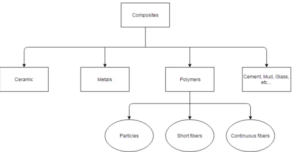
A composite material consists of a matrix material representing the continuous phase, which must ensure the connection of the reinforcements, and a reinforcement material, defined as the discontinuous phase, which provides resistance. The different types of composite materials are schematically represented in Figure 2-1.

(24)

2.1.1 Matrix

As can it be observed in Figure 2-1 the constituent material of the matrix can be ceramic, metals, polymers. Other common matrices include cement, mud and glass. Particularly, in aerospace industry, polymers as epoxy resin are used as a structural matrix material. The matrix material surrounds and supports the reinforcement materials by maintaining their relative positions and transferring loads among the reinforcements.

2.1.2 Reinforcement

The reinforcement provides strength and rigidity to the composite. Reinforced polymers can contain reinforcements in two different ways: Particles or Fibers, which can be short or continuous fibers, presented in Figure 2-2. Continuous fibers composites usually have better properties when compared with short fibers and particles composites, as the matrix does not transfer the loads between the reinforcement as often.

2.1.3 Lamina Stress-Strain Relationships

Stress-strain curves are an extremely important and often used graphical measure of a material’s mechanical properties. These curves are usually obtained with uniaxial tension test in which a strip or cylinder of the material anchored at one end and subjected

(25)

7 to an axial load [5]. As the load is increased gradually, the axial displacement is registered. Eventually the test specimen will fail when the ultimate tensile stress is reached.

In this test, it is possible to determine various mechanical properties of the material. The ultimate tensile stress mentioned above is the strength of the material i.e. the material’s resistance to failure by fracture. Another very important mechanical property is stiffness, which is the extent to which it resists deformation when applied to a certain load.

This relation, between the load 𝑃 and is resulting deformation 𝛿 is generally known as Hooke’s Law and it can be written as

𝑃 = 𝑘 ∗ 𝛿 (1)

Stiffness is the constant of proportionality_𝑘. However, the stiffness is also influenced by the specimen shape, therefore, in order to adjust the stiffness to be a purely material property, the load is normalized by the cross-sectional area and displacement 𝛿by the specimen’s original length [5]. Hooke’s Law can be written as

𝑃 𝐴0= 𝐸 ∗

𝛿 𝐿0

(2)

or

𝜎 = 𝐸 ∗ 𝜀 (3)

(26)

Equation 3 is the stress _𝜎 - strain _𝜀 relationship, represented in Figure 2-3 (b), and the constant of proportionality _{𝐸, commonly known as Young’s modulus or modulus of} elasticity, is one of the most important mechanical descriptors of a material. The Young’s modulus is a measure of a material’s stiffness; a stiff material needs a bigger load to deform when compared to a soft material. Nonetheless, the Young’s modulus can have various values according to the direction of loading.

An isotropic material has identical values of a certain property in all directions, therefore, it has the same strain regardless of the direction of the load applied.

An anisotropic material, such as CFRP, is directionally dependent, which means it has a different strain according to the direction of the load applied.

An orthotropic material is a subset of anisotropic materials as it has three mutually perpendicular planes of symmetry. Transversely isotropic materials, such as unidirectional carbon fibers, are special orthotropic materials that have one axis of symmetry. This means, generally, CFRP have greater stiffness in the direction of the fibers than in the transverse and thickness directions. The fibers can be aligned randomly within the material, but it is desirable to orientate them preferentially in the direction of the highest applied load.

Most CFRP applications are subjected to loads in different directions and controlling the material’s anisotropy is an important mean of optimizing the material for specific applications.

(27)

9 2.1.4 Textile Reinforced Composites (TRC)

Textile Reinforced Composites consist of composite materials with textiles as reinforcements and polymers as matrix. The development of this particular composite is based on the necessity to control the anisotropy of the fibers. Textiles can be designed so that the fibers are placed on preferential directions as most structures are loaded in multiple directions. TRC have applications in various fields; and, particularly in aeronautic industry, with high economic impact.

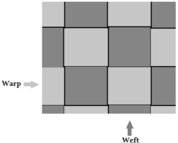
According to Tong, Mouritz and Bannister [6], the main processes used in the production of textile composites are: Weaving, Braiding, Knitting and Stitching. Weaving consists in producing a fabric by interlacing the threads of the weft and the warp on a loom, as shown in the Figure 2-4. Woven fabrics will be the focus of study in this dissertation.

Mechanical properties of the material can be affected by various parameters, such as yarn’s dimension and spacing, weave architecture or yarn’s fiber volume fraction [3].

Figure 2-5 shows different patterns of 2D woven fabrics. In this dissertation, it will be studied a plain weave pattern.

(28)

Pre-preg textile

Pre-preg is the most common term to describe composite fibers that are already pre-impregnated with a matrix material, such as an epoxy resin. The matrix is partially cured to allow easy handling and, after lay-up, requires a cure in an oven or autoclave. The pre-preg is cut and laid up, by hand or machine, layer by layer, to produce a laminate with the desired orientations and number of plies [1].

In this dissertation, the models consist of plain weave patterns of carbon fibers pre-impregnated in an epoxy resin, with 26 plies. However, the material used in this dissertation is not a conventional carbon fabric and will be discussed ahead.

Spread Tow Carbon Fabric

As mentioned before, in order to improve the mechanical properties, developments in TRC have been made. Besides the necessity to control the anisotropic behaviour of the fibers, there is a demand for lighter structures. El-Dessouky and Lawrence [7] studied a method, using tow-spreading technology to achieve ultra-lightweight thermoplastic composites. It consisted in thinning a conventional carbon fiber by increasing the tow width from 5 mm to 25 mm. The authors reported the laminate had improved mechanical properties, lower void content and displayed better fiber packing.

(29)

11 The Figure 2-6 is a representative cross-section of a plain weave with regular tows when compared with a plain weave with spread tow. The material used in this dissertation will be a plain weave spread tow carbon fabric.

2.2 Damage in Composite Materials

Consider a fibre reinforced plastic unidirectional and unnotched lamina. When submitted to plane stress states, the material can sustain a load limit. Surface failure is a 3D stress surface of all the limit load points. Stress states beyond this surface, cause the material to lose his structural integrity whereas the stress states inside the failure surface do not. Failure criteria are analytical functions that represent the surface failure and some of the most popular failure criteria are presented ahead.

In unidirectional laminates, there are five possible uniaxial tests:  Fibre direction tension and compression test_(𝜎₁₁₎;  Transverse tension and compression test_(𝜎₂₂₎;  In-plane shear stress test _(𝜎₁₂₎;

For each uniaxial test there is a failure tension associated, represented in Figure 2-7 as_𝑋_𝑇,_𝑋_𝐶,_𝑌_𝑇,_𝑌_𝐶 and _𝑆_𝐿, respectively.

2.2.1 Laminated failure modes

According to Maimí [8], in unidirectional laminates under plane stress states, there is, at least, four failure modes clearly identified, as shown in Figure 2-7.

Figure 2-6 - Representative cross-section of a plain weave with regular tows (on top)

(30)

Longitudinal fracture: 𝜶 = 𝟎°

The fracture occurs longitudinally (_{𝛼 = 0°}) to the laminate. It should be noted that this failure mode occurs either with transverse tension and in-plane shear stress or with high in-plane shear stresses and moderate transversal compression.

This failure mode corresponds to the Figure 2-7 (c) and _𝛼 is the angle between the fracture and axis 3.

Longitudinal fracture: 𝜶 ≠ 𝟎°

As mentioned above, with high in-plane shear stresses and moderate transversal compression, the failure occurs longitudinally to the laminate. However, according to Puck and Schürmann [9], increasing the transversal compression, the angle _𝛼 changes to approximately _40°. Actually, under a pure transverse compression test, the angle _𝛼 changes to approximately_{53° ± 3°}.

(

Figure 2-7 – Surface failure and different failure modes [8].

(a)

(b)

(c)

(31)

13 This failure mode is represented in the Figure 2-7 (d).

The influence of in-plane shear stress in the fracture angle is very curious. In a unidirectional laminate under transverse compression, it is observed that the fracture angle decreases with the intensity of the in-plane shear stress until the failure occurs longitudinally to the laminate.

Longitudinal Tensile Failure Mode

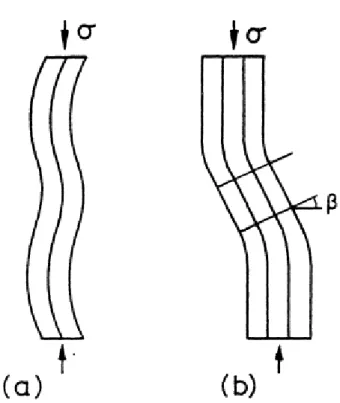
Under longitudinal tension, the failure occurs transversally to the laminate, as it can be seen in the Figure 2-7 (a). It is the simplest failure mode because the reinforcement properties dominate. The majority of the load is transferred to the fibers and, when they fail, due to local defects, the stress is distributed increasing the tension to the other fibers. These tensile stresses are transferred as shear tensions between the interface and the matrix causing cracks in the matrix and debonding.

Simple failure criteria as maximum tension or maximum strain to predict failure are appropriate for longitudinal tension damage.

Longitudinal Compression Failure Mode

At last, the most complex failure mode occurs under longitudinal compression. There are several competing mechanisms of longitudinal compressive failure: 1) the generation of a kink band is the most common, 2) microbuckling or 3) fiber crushing. For example, aramid fibers have low compression resistance and are serious candidates to fiber crushing; however, this failure mode is not common in composites.

(32)

As stated by Maimí [8], there are still some debates about the formation of a kink band, either it is a failure mechanism by itself or it is the last stage of microbuckling. However, the geometry of a kink band is not similar to buckling and the author considers that the formation of a kink band begins with the excessive rotation or destabilization of an initially misaligned fiber. Consequently, the matrix and interface must transfer high in-plane shear stresses contributing to damage, matrix fracture and component separation.

2.2.2 Fracture mechanism

The study of the propagation of cracks in materials is commonly known as Fracture mechanics, a field of mechanics. It is an important tool to improve mechanical performance of mechanical components.

Early approaches tried to predict fracture by investigating the behaviour of atomic bonds. However, in theory, the theoretical stress need to break the atomic bonds was much higher than the experimental results. Therefore, Griffith suggested that the discrepancy between theoretical and experimental fracture stress was due to the presence of microscopic flaws or defects in the material.

(33)

15 In order to verify the flaw hypothesis, Griffith introduced and solved an idealized problem of a single artificial crack in an infinite two-dimensional, isotropic, elastic medium under transverse load [3]. The prediction of crack growth is based on an energy balance. A crack growth will occur where there is enough energy available to generate new crack surface [11]. Applying the energy balance principle, the solution is given by

𝜎 = √2 ∗ 𝐸 ∗ 𝛾_{𝜋 ∗ 𝑎}

(4)

where a is the half artificial crack length, _𝜎 is the stress that causes the crack growth unstable under plane stress conditions and _𝛾 represents the classical surface energy due to the breakage of bonds in the generation of new crack surface.

Following Griffith’s work, Irwin introduced the macroscopic energy release rate, 𝐺, associated to the behaviour of cracks. A crack growth has three different modes and each of these modes has its critical energy 𝐺𝐼𝑐, 𝐺𝐼𝐼𝑐 and 𝐺𝐼𝐼𝐼𝑐. The failure propagation modes and its respective critical energy are explained in detail in the Chapter 3.2, in which they are used to simulate delamination between plies and to characterize the interface material. The energy release rate is given by

𝜎 = √𝐸 ∗ 𝐺_{𝜋 ∗ 𝑎}

(5)

where,

𝐺 =𝛿𝑈 𝛿𝐴

(6)

(34)

2.2.3 Shear Plasticity

As it was mentioned in Chapter 1.1, one of the goals for this dissertation is the incorporation of a plasticity model. In this chapter it will be described the composite materials’ behaviour under different arrangements and explained the need to incorporate a plasticity model and the reason why the previous dissertation did not have one. In unidirectional laminates as the one in the Figure 2-7, due to their geometry five uniaxial tests can be made, longitudinal tension and compression, transversal tension and compression, and shear stress test.

(35)

17 According to Maimí [8], it is reasonable to assume the composite has elastic behaviour until failure except in shear stress and transversal compression stress as they are clearly non-linear. Furthermore, Koerber, Xavier and Camanho [12] performed quasi-static and dynamic experiments for off-axis and transverse compression specimens. The results are shown in Figure 2-9.

Analysing Figure 2-9, in pure _(90°) transverse compression, despite showing a slight non-linearity response it is acceptable to admit there is no plasticity.

Decreasing the angle, from 75° to 45° there is a clear increasing non-linear response. It should be noted that off-axis loads are a combination of shear and transverse compression loads and the maximum shear stress occurs when the off-axis angle is _45°[13].

Decreasing even further the angle, from _45°to_15°, as the shear stresses diminish, as it can be evidenced in the Figure 2-9, there is an increasing linearity in the response.

Consider the numerical model developed in the previous dissertation. As it only studied a _0°/90° arrangement, the meso-scale model is subject to transverse and longitudinal tensile loads and therefore there was no need to incorporate a plasticity model as it is more complex and has many solution convergence problems.

2.3 Failure Criteria for CFRP Laminates

As mentioned before, failure criteria are analytical functions that represent the surface failure and predict if a material will fail under the action of external loads. There has been a lot of research in this area, however there is still no universally accepted criterion by the scientific community under general load conditions.

(36)

2.3.1 Failure criteria not associated with failure modes

In this group, the expressions that represent the surface failure are functions of the material strengths. These expressions are a result of a polynomial adjusting to experimental results and ignore the different failure modes of composite materials.

An evident advantage of these criteria is their invariance under rotation of coordinates; however, they do not take into account the lack of homogeneity of the composite material.

Tensor Polynomial Criterion (Tsai-Wu Criterion)

Commonly known as Tsai-Wu Criterion, a general polynomial failure criterion that is expressed as:

𝐹𝑖∗ 𝜎𝑖+ 𝐹𝑖𝑗∗ 𝜎𝑖∗ 𝜎𝑗+ 𝐹𝑖𝑗𝑘∗ 𝜎𝑖∗ 𝜎𝑗∗ 𝜎𝑘 ≥ 1 (7)

Several other criteria have been proposed, variations of the general Tsai-Wu criterion in order to ensure a better fit to the experimental results such as Tsai-Hill, Axxi-Tsai, Hoffman and Chamis [14].

2.3.2 Failure criteria associated with failure modes

In this group, the expressions take into account the non-homogeneity of composites and are able to predict the different failure modes: Fiber fracture, Transverse Matrix Cracking and Shear Matrix Cracking [14].

(37)

19 Maximum Strain Criterion

The failure occurs when the strain exceeds a specific value, therefore when one or more equations are not satisfied. Three different functions are used to predict the different failure modes.

Fiber: _𝜀₁_{≥ 𝜀}_1𝑇𝑢 _or _|𝜀

1| ≥ 𝜀1𝐶𝑢 (8)

Matrix: _𝜀₂_{≥ 𝜀}_2𝑇𝑢 _or _|𝜀

2| ≥ 𝜀2𝐶𝑢 (9)

Shear: _𝜀₁₂_{≥ 𝜀}₁₂𝑢 ₍₁₀₎

𝜀1𝑇𝑢 , 𝜀2𝑇𝑢 , 𝜀1𝐶𝑢 , 𝜀2𝐶𝑢 : - normal failure strain of the lamina in the 1 and 2 direction, under tension and compression, respectively.

𝜀12𝑢: - shear failure strain of the lamina in the 12 plane.

𝜀1 , 𝜀2 , 𝜀12 - strains in the directions 1, 2 and 12, respectively.

Maximum Stress Criterion

Similar to the Maximum Strain Criterion, the failure occurs when the stress exceeds a specific value, therefore when one or more equations are not satisfied.

Fiber: _𝜎₁_{≥ 𝜎}_1𝑇𝑢 _or _|𝜎

(38)

Matrix: _𝜎₂_{≥ 𝜎}_2𝑇𝑢 _or _|𝜎

2| ≥ 𝜎2𝐶𝑢 (12)

Shear: 𝜎12≥ 𝜎12𝑢 (13)

𝜎1𝑇𝑢, 𝜎2𝑇𝑢, 𝜎1𝐶𝑢, 𝜎2𝐶𝑢 : - normal strength of the lamina in the 1 and 2 direction, under tension and compression, respectively

𝜎12𝑢: - normal shear strength of the lamina in the 12 plane

𝜎1 , 𝜎2 and 𝜎12 - stresses in the directions 1, 2 and 12 respectively

Hashin-Rotem Criterion

This criterion only takes into account the fiber failure and matrix failure, nevertheless it is made a distinction between tension and compression.

Fiber: _𝜎₁_{= 𝜎}_1𝑇𝑢 _if _𝜎

1 > 0 −𝜎1= 𝜎1𝐶𝑢 if 𝜎1 < 0

(14)

Matrix

(𝜎2 𝜎_2𝑇𝑢)

2 + (𝜎12

𝜎₁₂𝑢) 2

= 1 if _𝜎₂ _{> 0}

(𝜎2 𝜎_2𝐶𝑢)

2 + (𝜎12

𝜎₁₂𝑢) 2

= 1 if _𝜎₂ _{< 0}

(15)

𝜎1𝑇𝑢, 𝜎2𝑇𝑢, 𝜎1𝐶𝑢, 𝜎2𝐶𝑢 : - normal strength of the lamina in the 1 and 2 direction, under tension and compression, respectively

𝜎12𝑢: - normal shear strength of the lamina in the 12 plane

(39)

21 LaRC03

LaRC03 is a recently developed set of six phenomenological criteria proposed by Dávila, Camanho and Rose [15] for predicting failure of unidirectional FRP laminates. It is based on Hashin and Puck’s fracture plane concepts. This failure criterion can predict matrix and fiber failure accurately for in-plane stress states.

Criterion for Matrix Failure Under Transverse Compression – LaRC03#1

This failure mode is explained in detail in Chapter 2.2.1.2 and represented in Figure 2-7 (d). This criterion is based on the Mohr-Coulomb (M-C) criterion, Mohr’s circle represented in Figure 2-11 for a state of uniaxial compression, and the matrix failure index is given by the following expression:

LaRC03#1 _𝐹𝐼_𝑀_{= (}𝜏𝑒𝑓𝑓

𝑇

𝑆𝑇 ) 2

+ (𝜏_𝑆𝑒𝑓𝑓𝐿 𝐿𝑖𝑠

) 2

≤ 1 (16)

(40)

The subscript ’M’ indicates matrix failure and ‘is’ indicates that, for general laminates, the in situ longitudinal shear strength should be used rather than the strength of a unidirectional laminates. The transverse and longitudinal shear strengths are represented by _𝑆_𝑇 and _𝑆_𝐿_𝑖𝑠, respectively. Generally, the fracture plane can be subjected to transverse as well as in-plane stresses therefore the effective stresses must be defined in both orthogonal directions, given by the following expressions.

𝜏_𝑒𝑓𝑓𝑇 _{= 〈|𝜏}𝑇_{| + 𝜂}𝑇_{∗ 𝜎}

𝑛〉 (17)

𝜏𝑒𝑓𝑓𝐿 = 〈|𝜏𝐿| + 𝜂𝐿∗ 𝜎𝑛〉 (18)

The terms _𝜂𝑇_and_𝜂𝐿_{are commonly known as coefficients of transverse and} longitudinal influence, respectively and they are represented in Figure 2-11. This criterion is detailed explained in the article [15].

Criterion for Matrix Failure Under Transverse Tension – LaRC03#2

In Chapter 2.2.1.1, it is briefly explained this failure mode and it is represented in Figure 2-7 (c). According to Dávila, Camanho and Rose [15], this failure mode normally causes a small reduction in the overall stiffness of a structure, nevertheless, it affects the development and propagation of damage and it provides the primary leakage path for gases in pressurized vessels. The matrix failure index is now given by the following equation.

LaRC03#2 _𝐹𝐼_𝑀_{= (1 − 𝑔) ∗}𝜎22

𝑌_𝑖𝑠𝑇 + 𝑔 ∗ ( 𝜎22

𝑌_𝑖𝑠𝑇) 2

+ (𝜏_𝑆12 𝑖𝑠𝑇)

2

≤ 1 (19)

The in situ transverse tensile and longitudinal shear strengths are represented by 𝑆𝑇 and 𝑆𝐿𝑖𝑠, respectively. The term 𝑔 is a material constant and it is given by quotient between Mode I and Mode II energy release rates.

𝑔 =_𝐺𝐺𝐼𝑐

(41)

23

Criterion for Fiber Tension Failure – LaRC03#3

This failure criterion is associated with the failure mode explained in Chapter 2.2.1.3 and it is represented in Figure 2-7 (a). It is simple to measure and it is independent of fiber volume fraction and Young’s modulus [15]. Therefore, the failure index for fiber tensile failure is:

LaRC03#3 𝐹𝐼𝐹 =𝜀_𝜀11

1𝑇 ≤ 1 (21)

The subscript ’F’ indicates fiber failure.

Criterion for Fiber Compression Failure – LaRC03#4 and LaRC03#5

At last, these criteria this failure mode is explained in Chapter 2.2.1.4. It Is a complex failure mode and, for that reason, it has two different criteria. It can fail by the formation of a kink band and it can be predicted using the failure criterion for matrix tension or compression and ply stresses in the misalignment coordinate frame m. For matrix compression, _𝜎₂₂𝑚 _{< 0}_{, the criterion is the Mohr Coulomb criterion given in} Equation 16, LaRC03#1, with _{𝛼 = 0°} and _𝜏_𝑒𝑓𝑓𝑇 _{= 0}_{[15]. Consequently, the failure index} for fiber compression is:

LaRC03#4 𝐹𝐼_𝐹= 〈|𝜏12

𝑚_{| + 𝜂}𝐿_{∗ 𝜎} 22𝑚

𝑆_𝑖𝑠𝐿 〉 ≤ 1 (22)

For fiber compression with matrix tension it is used the matrix tensile failure criterion give in the Equation 19 with the transformed stresses. Hence, the other failure index for fiber compression is:

LaRC03#5 _𝐹𝐼_𝐹_{= (1 − 𝑔) ∗}𝜎22

𝑚

𝑌_𝑖𝑠𝑇 + 𝑔 ∗ ( 𝜎₂₂𝑚

𝑌_𝑖𝑠𝑇) 2

+ (𝜏_𝑆12𝑚 𝑖𝑠𝑇)

2

(42)

Matrix Damage in Biaxial Compression

According to Dávila, Camanho and Rose [15], it can still occur matrix damage without damage to the fibers or kink band formation. Hence, the failure index for matrix biaxial compression is calculated using the failure criterion in Equation 16, LaRC03#6, and the misaligned frame stresses:

LaRC03#6 _𝐹𝐼_𝑀_{= (}𝜏𝑒𝑓𝑓

𝑚𝑇

𝑆𝑇 ) 2

+ (𝜏_𝑆𝑒𝑓𝑓𝑚𝐿 𝐿𝑖𝑠

) 2

≤ 1 (24)

Now, the effective shear stresses are functions of the fracture angle , which can only be determined iteratively.

LaRC04

Similar to LaRC03, the LaRC04 criteria is also a recently developed set of six failure criteria that was developed taking into account the three-dimensional stress states including shear non-linearity. It was proposed by Pinho, Dávila, Camanho, Iannucci and Robinson [16]. According to the authors, LaRC04 is arguably better than most existing criteria and there is a correlation between his prediction and experimental results.

In order to apply the criteria, some material properties are required: The Young’s modulus _𝐸₁₁_{, 𝐸}₂₂, the in-plane shear modulus, _𝐺₁₂_{, the Poisson’s ratio, 𝜈}₁₂, the failure tensions, _𝑋𝑇_{, 𝑋}𝐶_{, 𝑌}𝑇_{, 𝑌}𝐶_{, 𝑆}𝐿_{and the critical energy release rates}_𝐺

𝐼𝑐, 𝐺𝐼𝐼𝑐.

The set of six failure criteria are somewhat complex and long-lasting, therefore, for more detailed information about each criterion, review Pinho, Dávila, Camanho, Iannucci and Robinson’s article [16].

(43)

25

Table 2.1 - Summary of the LaRC04 criteria (Adapted from [16])

Matrix Compressive Failure 𝜎₂₂< 0

LaRC04#5 _𝜎₁₁_{< −𝑌}𝐶 _LaRC04#2_𝜎

11≥ −𝑌𝐶

𝐹𝐼𝑀= ( 𝜏 𝑇𝑚 𝑆𝑇_{− 𝜂}𝑇_{∗ 𝜎}

𝑛𝑚) 2

+ (_𝑆 𝜏𝐿𝑚 𝑖𝑠𝐿 − 𝜂𝐿∗ 𝜎𝑛𝑚)

2

𝐹𝐼𝑀= ( 𝜏 𝑇 𝑆𝑇_{− 𝜂}𝑇 _{∗ 𝜎}

𝑛) 2

+ (_𝑆 𝜏𝐿 𝑖𝑠𝐿 − 𝜂𝐿∗ 𝜎𝑛)

2

Fiber Compressive Failure 𝜎₂₂< 0

LaRC04#4 _𝜎₂₂_{< 0} LaRC04#6 _𝜎₂₂ _{< 0}

𝐹𝐼𝑀= ( 𝜏1 𝑚₂𝑚 𝑆_𝑖𝑠𝐿 _{− 𝜂}𝐿_{∗ 𝜎}₂_𝑚₂_𝑚)

2

𝐹𝐼𝑀/𝐹= (1 − 𝑔)𝜎2 𝑚₂𝑚 𝑌_𝑖𝑠𝑇 + 𝑔 (

𝜎2𝑚₂𝑚 𝑌_𝑖𝑠𝑇 )

2

+Λ°23𝜏22𝑚3𝜓+ 𝜒(𝛾1𝑚2𝑚) 𝜒(𝛾12|𝑖𝑠𝑢 )

Matrix Tensile Failure 𝜎₂₂< 0 Fiber Tensile Failure 𝜎₂₂< 0

LaRC04#1 LaRC04#3

𝐹𝐼𝑀= (1 − 𝑔)_𝑌𝜎2 𝑖𝑠𝑇+ 𝑔 (

𝜎2 𝑌_𝑖𝑠𝑇)

2

+Λ°23𝜏232 + 𝜒(𝛾12) 𝜒(𝛾12|𝑖𝑠𝑢 )

𝐹𝐼𝐹=𝜎_𝑋11_𝑇

(44)

2.4 Different scale models

Continuum mechanics models study an object as a continuum, at a specific scale, therefore the problem variables can be described as continuum functions. FEM uses continuum mechanics, but the numerical model dimensions have a strong influence on the physical phenomena to be studied. As composites are constituted from two or more distinct materials, a simple approach would be to use a set of finite elements to represent each of these materials. However, even for a simple component, this could result in a prohibitive computational cost. Nevertheless, the use of different elements for dissimilar materials has the advantage of allowing the study of their interface behaviour, for instance.

Nowadays, when studying fiber reinforced composite material numerical models, several different scales can be considered, each one with their typical size, adequate to study specific phenomena and insufficient to study others, the most common being micro-scale, meso-scale and macro-scale. It is then convenient to choose the appropriated scale or dimensions according to the physical phenomena to be studied,

(45)

27 as shown in the Figure 2-12. It is also possible to create numerical models that consider two or more scales simultaneously, in a field known as Multi-Scale Modelling.

2.4.1 Micro-scale models

At the smallest scale usually used in composite numerical models, micro-scale, the concept of Representative Volume Element (RVE) is essential. According to Kanit, Forest, Galliet, Mounoury and Jeulin [17], “The RVE is usually regarded as a volume V of heterogeneous material that is sufficiently large to be statistically representative of the composite, i.e., to effectively include a sampling of all microstructural heterogeneities that occur in the composite.”

Using this scale, the model size is typically measured in _𝜇𝑚 and the mechanisms that trigger elasticity, stiffness reduction and plasticity can be studied. Figure 2-13 (a) represents a model created at this scale.

2.4.2 Meso-scale models

In this scale, the micro-scale phenomena can be handled as continuum just like the constitutive equations for the analysis. In Crespo’s master dissertation, meso-scale models were chosen for numerical simulation because these models have the ability to describe and predict damage and failure at the ply level as well [3]. As already stated in the objectives, in this dissertation, Crespo_{’ numerical model will be develop}ed for

(46)

different arrangements therefore, meso-scale models will be used as they are the most adequate models to this dissertation’s goal and they are represented in Figure 2-12 (b).

2.4.3 Macro-scale models

With the results of meso-scale model, it is possible to homogenize a whole structure or component and analyse their response under general loads. Macro-scale models, represented in Figure 2-12 (c), are incapable of predicting the interaction between fiber and matrix, nonetheless, they are computationally proficient in the simulation of real structures, like cars or planes, and are therefore vastly used in engineering [3].

2.5 Different arrangements

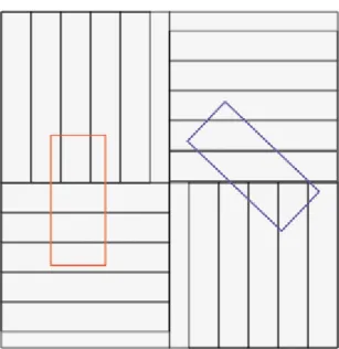
To better describer the different arrangements to be studied in this dissertation, a representative drawing was made and it is shown in Figure 2-14. As mentioned before, the material used in this dissertation will be a plain weave spread tow carbon fabric and the specimens are cut from the fabric with approximately_{10 ∗ 20 𝑚𝑚}2_{. The tow width is} 20 𝑚𝑚 and in the figure, it is presented the interlacing between horizontal fibers and vertical fibers.

(47)

29

2.6 Implicit & Explicit Analysis

2.6.1 Finite Element Method (FEM)

Virtually all physical phenomena can be described by physical laws and modelled through algebraic, differential or integral equations. An analytical description of a physical phenomenon is designated as a mathematical model and it can be defined as a set of equations that models the behaviour of the whole system through relations between variables and parameters that describe the system [18]. The analytical resolution for simple models is relatively easy to obtain whereas for complex models with complicated geometries, the resolution can be extremely difficult or even impossible.

However, the emergence of numerical simulation enabled the resolution of numerous engineering problems. Numerical simulation uses a computer and a numerical method to evaluate a mathematical model of a physical phenomenon. Nowadays there is an area of knowledge in expansion, known as computational mechanics, which is the

Figure 2-14 - A representation of this dissertation's composite material and different

(48)

development of mathematical models and numerical simulation in order to accurately models physical phenomena.

Among the numerical methods, there is one that stands out and it is a powerful tool to solve engineering problems _– the finite element method (FEM). It is a method adequate to solve problems of continuum mechanics. In FEM, the domain of the problem is decomposed in several sub-domains as it is based on the approximation of complex functions, for instance describing the displacement fields, with several simple polynomial functions. By controlling the number of sub-domains, we can achieve results with an error as slight as desired.

2.6.2 Static and Dynamic Analysis

Structural analysis studies the behaviour of a physical structure when subjected to a force or displacement. The distinction between dynamic and static analysis is in the acceleration that the action is applied. Static analysis is considered when the load is applied sufficiently slowly as the inertia forces can be ignored and the analysis can be simplified.

For dynamic analysis, the equilibrium equations including the deformation, the kinetic and damping dissipated energy are:

[𝑀] ∗ {𝑢̈} + [𝐶] ∗ {𝑢̇} + [𝐾] ∗ {𝑢} = {𝐹} (25)

In this equation,_{𝑀, 𝐶}and_𝐾are the mass, damping and stiffness matrices, respectively. Vector_𝐹is the applied forces in the nodes and_𝑢is the displacement vector. The vectors_𝑢̇and_𝑢̈are the first and second derivative of the displacement vector, that is, the velocity and acceleration vectors. As mentioned before, in static analysis the velocity and acceleration vectors can be ignored and the static equilibrium is given by the following equation:

[𝐾] ∗ {𝑢} = {𝐹} (26)

(49)

31 2.6.3 Difference between implicit and explicit analysis

Static analyses are done using implicit method, also known as the quasistatic method, whereas dynamic analysis can be done via explicit or implicit method. The main difference between both analyses is that implicit method implements Newton-Raphson iterations, whereas explicit method does not.

ANSYS uses the implicit method, that _{is based on Hooke’s law and energy balance} [19], which are more complex to program and require more computational effort in each solution step, however it allows larger time-step sizes. It is computationally expensive as the equation 14 is solved for _𝑢 and it requires a numerical solver to invert the stiffness matrix,_𝐾, once or even several times over the course of a load/time step.

On the other hand, LS-DYNA uses explicit analysis which can handle nonlinearities with relative ease when compared with implicit analysis. In this method the dynamic equilibrium equation 13 is solved for the acceleration, 𝑢,̈ which requires inverting the mass matrix, 𝑀, but it is trivial operation therefore each iteration is very efficient. However, in order to ensure solution stability, it requires several tiny time steps.

The explicit method is generally better in highly nonlinear problems in which the contact conditions change frequently, or high velocity impact problems where stress propagation wave effects are significant [19].

(50)

(51)

33

3 Numerical Analysis of CFRP

Plates

3.1 Mesh Generation

Finite element analysis goal is to recreate, mathematically, the behaviour of an actual engineering system. For that reason, it is extremely important that we generate a finite element model _– nodes and elements _– that adequately describe the model geometry. There are two methods to create a finite element model, solid modelling and direct generation.

(52)

Therefore, it is necessary to direct generate the location of each node and element “manually” hence the creation of a mesh generator algorithm. This algorithm, developed in Matlab, is a set of rules that are used to calculate and print the position of each nodes and assign these nodes to a specific element in the correct order. This guarantees not only the numerical model’s uniformity but also the guidance of the elements according to the fiber’s orientation. The algorithm is able to print this mesh for the software used in this dissertation, ANSYS, and for the software used in André Silva’s dissertation, LS -DYNA.

In the beginning of the mesh algorithm development, it was adopted the programming strategy as the central zone is relatively easier to model but the two extremities are more complex. The algorithm is divided by zone 1 _– the referential extremity, proceeding to the central zone and finishing in the other extremity. The element’s size is specified in the beginning of the algorithm but it is obtained through the number of complete finite elements in the z edge, represented as light blue in the Figure 3.1, and afterwards adapted the element’s size. E.g. in Figure 3.2, if the initially specified element size would result in ten and a quarter or half elements, the algorithm automatically adjusts the element size in order to have exactly ten elements in the z edge. _{This steps prevents a considerable element deformation in the specimen’s corner} and the size difference is redundant.

There is a node generation stoppage criterion in case the border’s element size becomes too small, e.g. if the node 30, represented in the Figure 3.2, is too close to the node 31, the criterion does not allow the node 30 to be generated and the element is now composed by the nodes 9,10,29 and 31.

(53)

35 Another criterion/rule is the specification of the number of lines that divide the zone 1, i.e. the imaginary lines that unite the nodes 21 to 27 and the nodes 28 to 31. It is chosen so that the elements are practically quadrangular being the edge’s size difference redundant.

Once created the nodes and elements in the zone 1, it is generated, following similar rules to the previous ones, the nodes until the other extremity of the specimen but, however, the nodes in the edge are not generated – afterwards they will be generated in order to maintain the mesh’s symmetry and not to overly deform.

In Figure 3.3, it can be seen the next step – the elements are created and the extremity still has no elements. In the algorithm, there is also the struggle to identify when it should create a quadrangular prism or degenerate them to triangular prisms. There are criteria that identify these situations and degenerates the prisms whenever necessary.

(54)

At last, the nodes and elements of the last zone are generated as well as the transition’s elements. The transition is random in the central zone, i.e. between the pink and light green lines, represented in the Figure 3.4.

This criterion was chosen in order to reduce the mesh’s and algorithm’s complexity. A little before or a little after would imply the transition beginning in the width area and finishing in the length area, as it can be seen in the dashed line represented in Figure 3.4.

Figure 3-3 – Triangular prisms detail.

(55)

37 The algorithm allows the user to:

 _{Choose the specimen’s arrangement direction:}0º/90º, 15º/-75º, 30º/-60º or 45º/-45º.

 Choose whether interface elements should be considered or not between the threads of weft and warp.

 Choose the element size.

 Choose the number of plies to be generated (1 to 26 plies).

 Choose in which software (ANSYS or LS-DYNA) the numerical model will be used.

The user picks these five parameters and the algorithm is fully capable of automatically generating the mesh with a random transition, that is, the location where the interlacing between the threads of warp and weft occurs, to replicate accurately how the experimental models are.

Figure 3-5 – 0º/-90º mesh

(56)

As shown in Figure 3-6, a 10-plies spread town carbon fabric model, it is detailed a 15º/-75º arrangement model and the random transition of each ply.

It should be noted that, when generating various plies, the algorithm also includes interface elements, discussed in Chapter 3.3, between each ply. There is also a more realistic option in the algorithm that includes interface elements between the weft and warp, to simulate the interaction between the weft and warp, however, in the dissertation, no models were studied with this option since it has a great computational cost and there was not enough time to develop this work. Nevertheless, it is an important future work to continue to develop this dissertation.

(57)

39

3.2 Interface Delamination Analysis

An interface exists whenever two materials are joined. The toughness and the ductility of composite structures, or in this case, CFRP plates are strongly dependent in the fracture or delamination along an interface between phases, which has stirred research on the failure of the interfaces. Delamination can be modelled by traditional fracture mechanics method, such as nodal release technique, or by techniques, such as cohesive zone material (CZM) model, that directly introduce fracture mechanisms.

In this chapter, in order to study interface delamination, it will be used CZM technology. Using ANSYS, there are two options to study this phenomenon: interface elements or contact elements. Both approaches introduce a failure mechanism by gradually degrading the material elasticity between surfaces and allow three modes of separation: mode I, opening mode, under normal stress, mode II, sliding mode, under tangential stress and mode III, a tearing mode, under tangential stress as shown in Figure 3-7. Each mode has associated a critical energy explained briefly in Chapter 2.2.2.

In order to validate the use of Cohesive Zone Modelling, specifically interface elements, a delamination numerical simulation analysis will be studied. Turon, Dávila, Camanho and Costa [20] have made an experimental analysis of a double cantilever beam specimen, schematically represented in Figure 3-8, and it is expected that ANSYS, using cohesive zone modelling, can reproduce the same results.

(58)

If that occurs, we can safely assume cohesive zone modelling can accurately simulate delamination and the interaction between the layers of the composite material. Cohesive zone damage models are characterized by the surface stresses (normal and tangential) and displacements (normal gap and tangential sliding), schematically represented in Figure 3-9, and the relation between them _{define the material’s behaviour.}

There are several constitutive laws that can be used in interface elements, however, in this analysis, the bilinear model will be used. It has two steps, a loading step and an unloading step, and in both of them, the stress-displacement relation is linear. The slope of the loading step is the interface stiffness,_𝐾, and the area under the stress-displacement relation is the fracture toughness, _𝐺_𝑐.

Figure 3-8 – Delamination of a double cantilever beam specimen.

(59)

41 3.2.1 ANSYS interface elements

In this thesis, delamination phenomenon will be simulated using interface elements, which have initially zero thickness, meshed between layers. ANSYS has four interface elements, two for 2D analysis – INTER202 (four nodes) and INTER203 (six nodes) - and two for 3D analysis _– INTER204 (sixteen nodes) and INTER205 (eight nodes).

In the continuation of Crespo’s [3] previous work, it was proven that the element SOLID185 (eight nodes brick element) with full integration provides good results with low computational cost and for that reason SOLID185 will be used along with INTER205 to model delamination in a double cantilever beam specimen

However, as shown before, in order to develop Crespo’s [3] numerical model with different and more complex specimen’s arrangements, it requires the direct generation of elements aligned with a certain angle, which leads to a necessity of creating triangular prisms in the edges. SOLID185 can be degenerated to a triangular prism with no contraindications but there is no information about degenerating interface element INTER205 and ANSYS displays a warning sign that does not allow the degeneration. It is possible to turn off ANSYS warnings to degenerate INTER205, however in order to proceed with absolute certainty of reliable results, it will be demonstrated that degenerated interface element INTER205 provides results as good as the undegenerated INTER205. Therefore, in addiction to studying interface elements behaviour, it will be made a comparison between INTER205 brick and triangular prisms (normal and degenerated elements).

(60)

The delamination test (double cantilever beam, DCB) fabricated by Turon, Dávila, Camanho and Costa [20] was an unidirectional T300/977-2 carbon fiber reinforced epoxy laminate. The specimen was 150 mm long, 20 mm wide with two 1.98mm thick layers and it had an initial crack length of 55 mm. A displacement is applied at the crack tip, schematically represented in Figure 3-8, and it is recorded the variation of force applied as the displacement is being applied, as shown in Figure 3-11. The mechanical and interface material properties are shown in Table 3.1.

Table 3.1 – Mechanical and interface material properties of T300/977-2 [21].

𝐸11 𝐸22, 𝐸33 𝐺12= 𝐺13 𝐺23 𝜈12= 𝜈13

150 GPa 11 GPa 6 GPa 3.7 GPa 0.25

𝜈23 𝜎𝑚𝑎𝑥 𝐺𝐼𝑐 𝐺𝐼𝐼𝑐 = 𝐺𝐼𝐼𝐼𝑐

0.45 60 MPa 0.352.N/mm 1.45N/mm

To fully define _{the ANSYS’ bilinear cohesive zone material for interface element}s, there are some more material constants to be specified:_𝛿_𝑛𝑐_–_{normal displacement jump} at the completion of debonding - and _𝛼 - ratio of _𝛿_𝑛∗_to_𝛿

𝑛𝑐. In the literature, many different interface stiffness, _{𝐾 =}𝜎𝑚𝑎𝑥

𝛿𝑛∗ , have been proposed, however Camanho et al.[22] obtained good results for graphite/epoxy specimens using a value of ₁₀6_{𝑁/𝑚𝑚}3_.

𝛿𝑛𝑐 =2 ∗ 𝐺_𝜎 𝐼𝑐

𝑚𝑎𝑥 =

2 ∗ 352

60 ∗ 106= 11.73 ∗ 10−6𝑚

(27)

𝛼 =𝛿_𝛿𝑛∗ 𝑛𝑐 =

𝜎𝑚𝑎𝑥 𝐾 𝛿𝑛𝑐 =

60 ∗ 106 106_{∗ 10}9

11.73 ∗ 10−6 = 5.115 ∗ 10−3

(61)

43 Figure 3-11 shows the numerical results of the first, and simplified, FEM model simulations, in red and blue, and the experimental results, in black. As the coordinates of the experimental results from Turon, Dávila, Camanho and Costa article [20], are not specified, the black line is merely representative and approximate.

The brick element model was 1500 elements long and 1 element wide and thick. For the triangular prism, the brick was divided in two, making it 3000 elements long and 1 element wide thick. As it can be observed, the results are not reasonable, there is a significant discrepancy between bricks and triangular prisms elements and the simulations cannot depict the experimental results with precision, even though the triangular prims are surprisingly close. It is clear that it is necessary a mesh refinement in order to better study this delamination example.

It is possible that the elements used in the layers, the 8 nodes brick element, cannot reproduce acceptable results for a beam-bending test, unlike the 20 nodes element, which is expected to provide very accurate results. In the 8 nodes brick element, the displacement between the inferior and superior nodes is linear, consequently the stress – derivative of the displacement – is constant which is wrong as it is trivially known that stress is linear in beam bending. Hence, a series of numerical simulations were made to find a mesh size and number of elements per thickness suitable to simulate beam bending. Theoretically, for a cantilever beam submitted to a force at the tip, the displacement is given by the following equation:

(62)

𝛿 = _{3 ∗ 𝐼 ∗ 𝐸 ⇔}𝐹 ∗ 𝐿3

⇔ 𝛿 = 20 ∗ 1503

3 ∗ 20 ∗ 1.98₁₂ 3∗ 150000 ⇔

⇔ 𝛿 = 11.5944 𝑚𝑚

(29)

In the numerical simulations, it was considered_{𝐹 = 20𝑁}, _{𝐸 = 150 𝐺𝑃𝑎} and the same dimensions of the previous specimen. Two studies were conducted, the effect of the number of elements per thickness - Thickness effect - and the effect of the number of elements long _– Length effect. In both studies it is compared the 20 nodes element results, the 8 nodes element result and the theoretical displacement.

(63)

45 As expected, it is clear that the 8 nodes element behaves poorly in beam bending, unlike the 20 nodes element, and only after some mesh refinement, especially in the number of elements per thickness, it converges to the solution.

Consequently, the mesh was refined in order to perform a final simulation for the double cantilever beam test to validate cohesive zone modelling in ANSYS. In the new mesh, each layer is 2 elements thick, 8 elements wide and 1500 elements long.

As it was expected, after refining the mesh, the simulation results converge to the experimental results. It can be concluded that the interface element INTER205 and element SOLID185, after some mesh refinement, yield very similar results as the experimental test. The initial results discrepancy was due to SOLID185 poor bending analysis, at least in the brick form. In addition, it can be safely assumed that the 8 node