Bayesian Estimation of Inefficiency Heterogeneity in
Stochastic Frontier Models
∗
Jorge E. Gal´
an
†Helena Veiga
‡Michael P. Wiper
§ABSTRACT
Estimation of the one sided error component in stochastic frontier models may erroneously attribute firm characteristics to inefficiency if heterogeneity is unaccounted for. However, it is not clear in general in which component of the error distribution the covariates should be included. In the classical context, some studies include covariates in the scale parameter of the inefficiency with the property of preserving the shape of its distribution. We ex-tend this idea to Bayesian inference for stochastic frontier models capturing both observed and unobserved heterogeneity under half normal, truncated and exponential distributed inefficiencies. We use the WinBugs package to implement our approach throughout. Our findings using two real data sets, illustrate the relevant effects on shrinking and separating individual posterior efficiencies when heterogeneity affects the scale of the inefficiency. We also see that the inclusion of unobserved heterogeneity is still relevant when no observable covariates are available.
JEL classification: C11; C23; C51; D24
Keywords: Stochastic Frontier Models; Heterogeneity; Bayesian Inference.
I. Introduction
Stochastic frontier models, first introduced in Aigner et al. (1977) and Meeusen and van den Broeck (1977), are important tools for efficiency measurement. These models require the speci-fication of an economic, functional form based on a production or cost function which includes
∗The authors would like to thank Mark Steel and Jim Griffin for their comments and suggestions as well
as the participants of the 33th National Congress on Statistics and Operations Research and the Permanent Seminar on Efficiency and Productivity of Universidad de Oviedo. Financial support from the Spanish Ministry of Education and Science, research projects ECO2009-08100, MTM2010-17323 and SEJ2007-64500 is also gratefully acknowledged.
†Department of Statistics, Universidad Carlos III de Madrid, C/ Madrid 126, 28903 Getafe, Spain. Email:
[email protected]. Corresponding author.
‡Department of Statistics and Instituto Flores de Lemus, Universidad Carlos III de Madrid, and BRU/UNIDE,
Avenida das For¸cas Armadas, 1600-083 Lisboa, Portugal.
a composite error term. This error term can be decomposed into two parts, firstly a two-sided, idiosyncratic error and secondly, a non-negative inefficiency component. Measures of efficiency are obtained from this one-sided error, which typically is assumed to follow some specific dis-tribution. The most common distributions for the one-sided error are the half-normal (Aigner et al., 1977), exponential (Meeusen and van den Broeck, 1977), truncated normal (Stevenson, 1980), and gamma (Greene, 1990).
However, the estimated inefficiency component often includes some firm characteristics other than outputs, inputs, or prices defined from the production or cost function, which should not be attributed to inefficiency. These firm characteristics are exogenous variables (e.g. type of ownership, GDP level in the country of operation) that have an effect on the technology used by the firms or directly on their inefficiency. If these variables are not taken into account in the model specification, this may affect the estimation of the inefficiencies or of the frontier significantly. The distinction between heterogeneity and inefficiency has become a very important issue in stochastic frontier models.
Firm characteristics can be modeled in the frontier if they imply heterogenous technologies or in the one-sided error component if they affect the inefficiency. In the former case, covariates are directly included in the functional form and the main interest is to model unobserved het-erogeneity (see Greene, 2005). For the case of hethet-erogeneity in the inefficiency, covariates are usually included in the parameters of the one-sided error distribution (see Huang and Liu, 1994). Heterogeneity in stochastic frontier models has also been studied from the Bayesian con-text. The Bayesian approach to stochastic frontiers introduced by van den Broeck et al. (1994) presents advantages in terms of formally deriving posterior densities for individual efficiencies, incorporating economic restrictions, and in the easy modeling of random parameters through hi-erarchical structures. Hihi-erarchical models have been used to capture heterogeneous technologies (see Tsionas, 2002) and heterogeneity in the inefficiency has been considered through covariates in the distribution of the non-negative error component (see Koop et al., 1997). Modeling ob-served heterogeneity using non parametric and flexible mixtures of inefficiency distributions are
other interesting recent contributions (see Griffin and Steel, 2004, 2008). However, the treatment of unobserved heterogeneity in the non-negative error component has been little explored.
Here, we propose the modeling of both observed and unobserved heterogeneity in the ineffi-ciency within a Bayesian framework. In particular, we extend the model of Caudill et al. (1995), where in the classical context, observed covariates were included in the scale parameter of a half normal inefficiency distribution. This model has the property of changing the scale while preserving the shape of the inefficiency distribution. This is called the scaling property in Wang and Schmidt (2002) and Alvarez et al. (2006) and allows us to think of the inefficiency as being composed of two parts where the first component captures random managerial skills and the second depends on firm characteristics. Here, we include heterogeneity in the parameters of half normal, truncated normal and exponential distributed inefficiencies in such a way that they are allowed to vary over time and that the scaling property is preserved.
For illustration, we use two data sets which have been previously analyzed only in the classical context. The first data set is from a controversial report by the World Health Organization (WHO) on the efficiency of national health systems (see WHO, 2000), while the second evaluates the economic efficiency of US domestic airlines. Results are compared against a base model with no heterogeneity and a model with covariates in the frontier.
The rest of this paper is organized as follows. Section II presents a brief literature review on heterogeneity in stochastic frontier models and the proposed model. Section III presents the Bayesian inference and model selection criteria. Section IV reports the applications to the WHO and the US domestic airlines data sets. Finally, in Section V we provide conclusions and consider some possible extensions of our approach.
II. Heterogeneity in stochastic frontier models
A. A brief literature review
The original stochastic frontier model introduced by Aigner et al. (1977) and Meeusen and van den Broeck (1977) has the following form:
yit = xitβ + vit− uit (1)
where yit represents the output for firm i at time t, xit is a vector that contains the input
quantities used in the production process, vit is an idiosyncratic error that is typically assumed
to follow a normal distribution and uitis a one-sided component representing the inefficiency and
following some non-negative distribution.
However, firm specific factors not specified in (1) can be mistaken for inefficiency if they are not identified. Heterogeneity can either shift the efficiency frontier or change the location and scale of the inefficiency estimations (see Kumbhakar and Lovell, 2000; Greene, 2008, for complete reviews). In general, when external factors are supposed to capture technological differences and these are out of the firms’ control, heterogeneity should be specified in the frontier. In this case, the main interest is capturing unobserved effects. In the classical context, this has been modeled through fixed and random effects or models with random parameters (see Greene, 2005). Bayesian approaches have been based on frontier models with hierarchical structures (see Tsionas, 2002; Huang, 2004).
When heterogeneity is more related to efficiency and thus more likely to be under firms’ control, then this should affect directly the one-sided error term. In the parametric context, inefficiency heterogeneity is often included in the location or scale parameters of the inefficiency distribution. For example, covariates shift the underlying mean of inefficiency in Kumbhakar et al. (1991), Huang and Liu (1994) and Battese and Coelli (1995). A reduced form of these models assumes that the location parameter of uit depends on a vector of covariates zit and
parameters δ as follows:
uit = |Uit|; Uit ∼ N (µit, σu2)
µit= zitδ.
(2)
The scale parameter of the one-sided error component has also been modeled as a function of firm characteristics. Reifschnieder and Stevenson (1991) provided one of the first linear spec-ifications where this parameter varies across firms. A similar model was proposed by Caudill et al. (1995) with the aim of treating heteroscedasticity in frontier models. These authors found biased inefficiency estimations when heteroscedasticity was not accounted for.1 The proposed
model specifies the variance of a half normal distributed inefficiency as an exponential function of time invariant covariates:
ui = |Ui|; Ui ∼ N (0, σ2Ui)
σUi = σU· exp(ziγ).
(3)
This specification has the characteristic of changing the scale of the inefficiency distribution while preserving its shape and is referred in the literature as the scaling property (see Wang and Schmidt, 2002; Alvarez et al., 2006). In general, this property allows us to think about inefficiency as being composed of two parts: uit = u∗it· f (zit, δ). The first component is a base inefficiency,
which is not affected by firm characteristics and captures random managerial skills, while the second component is a function of heterogeneity variables determining how well management is performed under these conditions. Another interesting feature of this property is that the interpretation of the effects of covariates on the inefficiency is direct and independent of the inefficiency distribution. The scaling property also holds when the inefficiency is exponentially distributed (see Simar et al., 1994), or in a particular case of truncated normal inefficiency where both parameters are an exponential function of firm characteristics as follows (see Wang and Schmidt, 2002; Alvarez et al., 2006):
uit = |Uit|; Uit ∼ N (µit, σU2it)
µit= µ · exp(zitδ)
σUit = σU · exp(zitδ).
(4)
Specification (4) for the inefficiency is a variation of a previous proposal by Wang (2002) where both the mean and the variance of truncated normal inefficiencies are simultaneously affected by the same covariates but with different coefficients. Other authors have also proposed heterogeneity specifications that include firm characteristics in the variance of the idiosyncratic error with the aim of treating heteroscedasticity in frontier models (see Hadri, 1999).
In the Bayesian context, Koop et al. (1997) presented different structures for the mean of the inefficiency component as Bayesian counterparts to the classical fixed and random effects models. One of these specifications is the varying efficiency distribution model, which includes firm specific covariates in the parameter of an exponential distribution. These covariates link the firm effects and only the efficiencies of firms sharing common characteristics are drawn from the same distribution. The following is the specification where a time invariant inefficiency depends on a vector of binary covariates wit and parameters γ:
ui ∼ Ex(λ−1i )
λi = exp(wiγ).
(5)
The literature on modeling of unobserved firm characteristics in the inefficiency is still scarce. In the frequentist context, Greene (2005) proposed a model where the coefficients of the observed covariates are allowed to be firm specific and vary randomly. In the Bayesian framework, the marginally independent efficiency distribution model proposed by Koop et al. (1997) may capture unobserved inefficiency heterogeneity through exponentially distributed inefficiencies with firm specific mean λi and independent priors.
B. The Model
In this section, we present a general stochastic frontier model for panel data that allows the modeling of both observed and unobserved inefficiency heterogeneity and preserves the scaling property. Inefficiencies are assumed to follow: a) a half normal distribution, which is an an extension of the specification for the scale parameter in (3), b) a truncated normal distribution, which extends the scaled Stevenson model in (4), or c) an exponential distribution that can be seen as an extension of model in (5). The general model is:
yit = xitβ + zitδ + vit− uit
vit ∼ N (0, σ2); uit = |Uit|
a) Uit ∼ N (0, σU2 · (exp(hitγI1+ τitI2))2)
b) Uit∼ N (µ · exp(hitγI1 + τitI2), σU2 · (exp(hitγI1+ τitI2))2)
c) Uit∼ Ex(λ · exp(hitγI1+ τitI2)),
(6)
where zit is the vector of the observed heterogeneity variables that affect the technology; hit is
the vector of all covariates with effects in the scale of inefficiency; τit is an unknown parameter
which intends to capture time varying unobserved firm effects in the inefficiency; and, β, δ, and γ are vectors of the estimated parameters. I1 and I2 are indicator variables taking the value of
1 when either observed covariates or unobserved heterogeneity are accounted for, respectively. It is easy to extend this specification to a hierarchical model which also allows for additional, unobserved, firm effects in the technology. However, in practical applications, mean posterior efficiencies are found to be very close to 1 for almost all firms (see Huang, 2004; Tsionas, 2002, for similar results). From our point of view, these results are inconclusive as they do not allow us to get reliable efficiency rankings.
III. Bayesian inference
The use of Bayesian methods in stochastic frontier analysis was introduced by van den Broeck et al. (1994) and has become very common in recent applications. Bayesian approaches have various attractive properties and, in particular, restrictions such as regularity conditions are easily incorporated and parameter uncertainty is formally considered in deriving posterior densities for individual efficiencies.
All the models derived from the general specification in (6) are fitted by Bayesian methods. In order to do this, we first need to introduce prior distributions for the model parameters. Here we assume proper but relatively disperse prior distributions throughout. The distributions assumed for the parameters in the frontier function are as follows: β ∼ N (0, Σ−1β ), δ ∼ N (0, Σ−1δ ) with diffuse, inverse gamma priors for the variances. Regularity conditions are imposed on those parameters in β that must be positive in order to satisfy the theoretical economic constraints on the frontier. Finally, the variance of the idiosyncratic error term is also inverse gamma, that is σ−2 ∼ G(aσ−2, bσ−2) with low values of the shape and scale parameters.
Regarding observed inefficiency heterogeneity, the distribution of the one-sided error compo-nent for the half-normal and truncated normal models are: u|γ, h ∼ N+(0, λ−1 · (exp(hγ))2),
and u|γ, h ∼ N+(θ · exp(hγ), λ−1· (exp(hγ))2), respectively; where the superscript + denotes
truncation to positive values, θ is the mean parameter, and λ is the precision parameter. For the exponential model the distribution is: u|γ, h ∼ G(1, λ · exp(hγ)), with shape parameter equal to 1 and scale parameter λ. For all models, γ is normally, N (0, Σ−1γ ) distributed with a diffuse prior for the covariance matrix. Parameters θ and λ are defined for each distribution as in Griffin and Steel (2007). Priors for these parameters are also valid in the case of models without heterogeneity in the inefficiency, where exp(hγ) = 1.
In the case of unobserved heterogeneity in the inefficiency, the unknown parameter is specified as: τ ∼ N (τ , σ−2τ ), where τ ∼ N (0, σ−2τ ) and σ−2τ ∼ G(aσ−2
τ , bσ−2τ ), with diffuse priors.
The complexity of these models makes necessary to use numerical integration methods such as Markov Chain Monte Carlo (MCMC), and in particular the Gibbs sampling algorithm with
data augmentation as introduced by Koop et al. (1995). For our models, implementation was carried out using the WinBUGS package following the general procedure outlined in Griffin and Steel (2007). For all our applications, the MCMC algorithm involved 50000 MCMC iterations where the first 10000 were discarded in a burn-in phase.
Finally, although we do not display the details here, we should also note that in our applica-tions, some sensitivity analysis of our results to changes in the prior parameters was carried out. Results showed that the posterior inference was relatively insensitive to small changes in these parameters.
A. Model selection
The different models are evaluated in terms of three criteria, the Deviance Information Criterion (DIC), the Log Predictive Score (LPS) and the Mean Square Error (MSE) of predictions. The former is a within sample measure of fit introduced by Spiegelhalter et al. (2002) commonly used in Bayesian analysis. Defining the deviance of a model with parameters θ as D(θ) = −2 log p(y|θ), where y are the data, then the DIC is
DIC = ¯D + pD
where ¯D is the expected deviance and pD is a complexity term such that pD = ¯D − D(¯θ), where
¯
θ is the mean of the posterior parameter distribution. The DIC can be evaluated automatically within the WinBugs setup and a good description of its use in stochastic frontier models can be seen in Griffin and Steel (2007).
The LPS is a scoring rule developed in Good (1952) and is defined as the average of log predictive density functions evaluated at observed out-of-sample values. In general, it compares the predictive distribution of a model with observations that are not used in the inference sample. To do this, we split the sample into two parts. The first set of n traininng data is used to fit the model and the predictive performance of the model is calculated on the second set of q data.
In our case, the training data set contains all observations except one for every firm, and the second data set just contains the last observation of every individual unit. In stochastic frontier frameworks, Griffin and Steel (2004) and Ferreira and Steel (2007) employed this criterion for model comparison. The formulation is the following:
LP S = −1 q
q
X
i=1
log p(yn+i|y1, ..., yn)
In this work, we also compare the models in terms of predictive mean squared error (MSE). This measure involves again the partition of the sample into two parts as above. The models are fitted using the training sample and their estimated parameters are used to predict the data for the last observation of every firm. The MSE is calculated as follows:
M SE = 1 k k X i=1 (yi− E [(β0xi− ui)|y1, . . . , yn]) 2 ,
where k is the number of firms, ui is the mean of the inefficiency component, which is different
depending on the distribution and varies with the firm for models with heterogeneity in the inefficiency.
IV. Empirical applications
In this section, we analyze two data sets, estimate the models presented in section II and interpret the results.
A. Application to WHO data set
Tandon et al. (2000) estimated the technical efficiency of 191 countries in the provision of health by using a classical fixed effects stochastic frontier model for an unbalanced panel. The original data set covers 5 years from 1993 to 1997 and the production function model proposed was the
following:
ln(DALEit) = αi+ β1ln(HExpit) + β2ln(Educit) + β3
1 2ln
2(Educ
it) + vit,
where DALE is the disability adjusted life expectancy, a measure that considers mortality and illness and represents health output. Input amounts are measured by HExp and Educ, which are health expenditure and the average years of education, respectively.
Their results were reported by the WHO and suffered from several criticisms since the authors did not consider the effects of heterogeneity in their study, even though the sample included countries with very different characteristics such as Switzerland, China, or Zimbabwe. This led to unexpected country health system performance rankings.
Greene (2004), using a classical random effects model, found that country rankings change when technology and inefficiency heterogeneity are considered. The author proposed to capture differences among countries by including eight exogenous variables separated into two groups: zi = [T ropicsi, P opDeni] and hi = [GEf fi, V oicei, Ginii, GDPi, P ubF ini, OECDi]. T ropics is
a binary variable that takes the value 1 if the country is located in the tropic and 0 otherwise; P opDen is the country population density, which may capture effects of dispersion but also congestion in the provision of health. GEf f is an indicator of government efficiency; V oice is a measure of political democratization and freedom; Gini is the income inequality coefficient; GDP is the per capita country gross domestic product; P ubF in is the proportion of health care financed with public resources, and OECD is a binary variable that takes the value 1 if the country belongs to the organization and 0 otherwise. Variables in zi are assumed to shift the
frontier itself and then they are included as covariates in the production function. Variables in hi
are more under the control of countries and policy related but it is not clear where they should be located.2
In order to assess the effects of heterogeneity under the Bayesian approach, we propose
2Greene (2004) chose a model with all covariates in the production function excluding Gini and GDP, which
four different models starting from our proposal in (6) using the covariates in zi and hi.3 The
inefficiency component may follow: a) half-normal, b) truncated normal, or c) exponential dis-tributions.
ln(DALEit) = α + β1ln(HExpit) + β2ln(Educit) + β312ln2(Educit) + β4T ropicsi
+β5ln(P opDeni) + hiδ + vit− uit
vit ∼ N (0, σv2); uit= |Uit|
a) Uit ∼ N (0, σU2 · (exp(hiγI1+ τitI2))2)
b) Uit ∼ N (µ · exp(hiγI1+ τitI2), σU2 · (exp(hiγI1 + τitI2))2)
c) Uit ∼ exp(λ · exp(hiγI1+ τitI2)).
(7)
The base model, denoted Model I, does not consider any type of heterogeneity in the in-efficiency, and only variables in zi are included in the production function. Model II includes
the covariates in hi as technology heterogeneity variables but not in the inefficiency. Therefore,
these two models assume I1, I2 = 0. Models III and IV incorporate our proposal of heterogeneity
that changes the scale but not the shape of the inefficiency. In particular, Model III allows the parameters of the inefficiency component to vary across countries through the random parameter τit that captures unobserved heterogeneity. For this model, δ = 0, I1 = 0 and I2 = 1. Finally,
Model IV captures observed heterogeneity in the inefficiency through covariates in hi and the
unknown parameter is omitted. Then, δ = 0, I1 = 1 and I2 = 0.4
Model comparison criteria for the four models and the three distributions are presented in Table I. In general, similar conclusions are obtained from the three criteria. Results show that models including either observed or unobserved heterogeneity improve from the base model. In particular, the model that exhibits the best fit and predictive performance includes observed heterogeneity in the inefficiency, which suggests that covariates in hi are inefficiency related.
Regarding the inefficiency distributions, the half-normal and truncated normal models present
3Regularity conditions are imposed on β
1 and β2.
4A model including observed and unobserved heterogeneity in the inefficiency parameters simultaneously was
also fitted but we omit the results because they were roughly the same as those obtained with Model IV. This could imply that the observed covariates in hi capture all relevant heterogeneity in the inefficiency.
Table I
Model comparison criteria assuming different inefficiency distributions Distribution Model I Model II Model III Model IV Half normal DIC -2251.7150 -2598.3080 -2423.3160 -2914.7370 LPS -97.1690 -132.7610 -154.8950 -196.4420 MSE 0.1382 0.0864 0.0906 0.0736 Truncated normal DIC -2292.7710 -2593.1280 -2495.1400 -2884.9030 LPS -122.8900 -130.4520 -146.7710 -185.9830 MSE 0.1387 0.1051 0.1084 0.0869 Exponential DIC -2223.7420 -2568.4380 -2231.4950 -2580.1720 LPS -95.9810 -121.5150 -123.3560 -132.2700 MSE 0.1392 0.1153 0.1281 0.1085
better indicators and seem to be better alternatives, specially for those models considering ob-served heterogeneity in uit. However, efficiency rankings are almost perfectly correlated across
distributions as we can observe for Model IV in Figure 1.
1 50 100 150 191 Exponential 1 50 100 150 191 1 50 100 150 191 H al f N or m al Truncated Normal
Figure 1. Efficiency rankings in Model IV across distributions
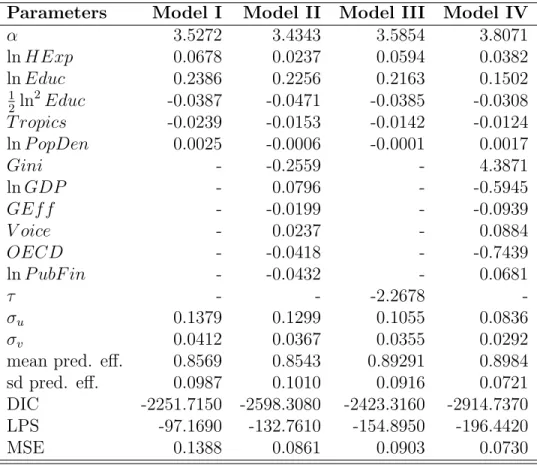
Hereafter, we report the results for the half-normal distribution given the better performance indicators obtained for model IV. Table II reports the mean of the posterior distributions of the parameters for the four models. In general, we observe that including covariates affecting the scale of the inefficiency component increases the mean and diminishes the dispersion of the predictive posterior efficiency. Regarding the coefficients, preserving the scaling property allows us to interpret directly the effect of covariates on the inefficiency in Model IV given that γ = ∂ ln uit/∂hi. We limit the analysis to the signs, which suggest that higher equality, income,
could be intuitively expected. In contrast, higher levels of democracy and public finance of health services lead to lower efficiency.
Table II
Posterior means of the parameter distributions with half-normal distributed inefficiency
Parameters Model I Model II Model III Model IV
α 3.5272 3.4343 3.5854 3.8071 ln HExp 0.0678 0.0237 0.0594 0.0382 ln Educ 0.2386 0.2256 0.2163 0.1502 1 2ln 2Educ -0.0387 -0.0471 -0.0385 -0.0308 T ropics -0.0239 -0.0153 -0.0142 -0.0124 ln P opDen 0.0025 -0.0006 -0.0001 0.0017 Gini - -0.2559 - 4.3871 ln GDP - 0.0796 - -0.5945 GEf f - -0.0199 - -0.0939 V oice - 0.0237 - 0.0884 OECD - -0.0418 - -0.7439 ln P ubF in - -0.0432 - 0.0681 τ - - -2.2678 -σu 0.1379 0.1299 0.1055 0.0836 σv 0.0412 0.0367 0.0355 0.0292
mean pred. eff. 0.8569 0.8543 0.89291 0.8984 sd pred. eff. 0.0987 0.1010 0.0916 0.0721 DIC -2251.7150 -2598.3080 -2423.3160 -2914.7370 LPS -97.1690 -132.7610 -154.8950 -196.4420 MSE 0.1388 0.0861 0.0903 0.0730
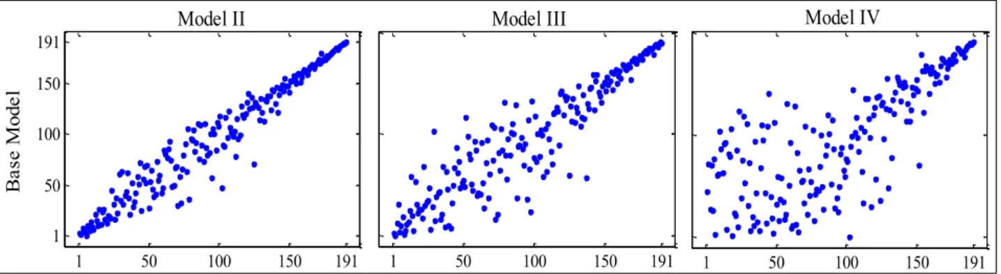
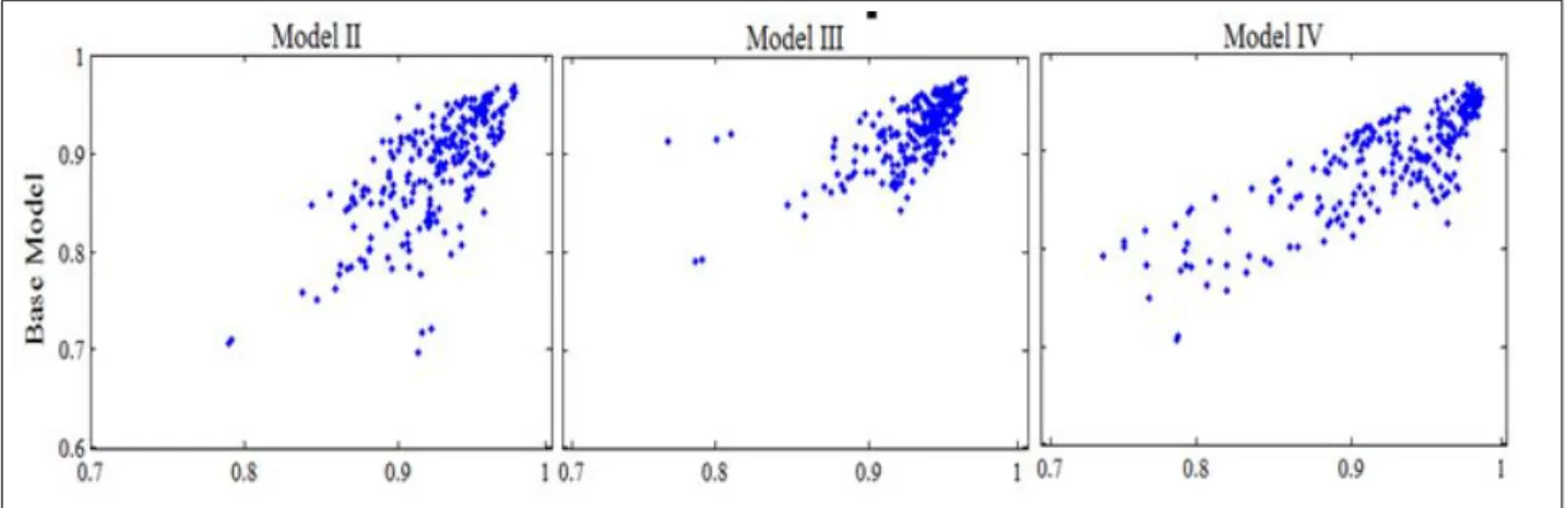
However, the most interesting conclusions come from the efficiency rankings since they allow for comparisons among countries. Figure 2 shows efficiency rankings’ scatter plots comparing the base model against the other three models. For Model II, which includes the covariates in the frontier, most countries preserve a similar position except for small changes in the middle rankings. The ranking correlation to the base model is 0.94. Model III, capturing unobserved heterogeneity in the inefficiency, shows a greater dispersion in middle positions but the first and last ranked countries barely change. The ranking correlation to the base model is 0.87. Finally, Model IV, the one with observed covariates in the scale parameter of the inefficiency, exhibits the greatest changes specially in top and middle positions, and presents the lowest
correlation against the base model (0.67). In particular, the highest ranked countries present major movements in their positions, specially when covariates are included in the inefficiency; while badly performing countries are always roughly the same regardless of the model used. This latter group is composed mainly of central African countries (e.g. Zambia, Botswana, Zimbabwe), which share some characteristics related to low income, tropical diseases, etc.
1 50 100 150 191 Model IV 1 50 100 150 191 Model III 1 50 100 150 191 1 50 100 150 191 B as e M od el Model II
Figure 2. Efficiency rankings - Base model vs. heterogeneity models
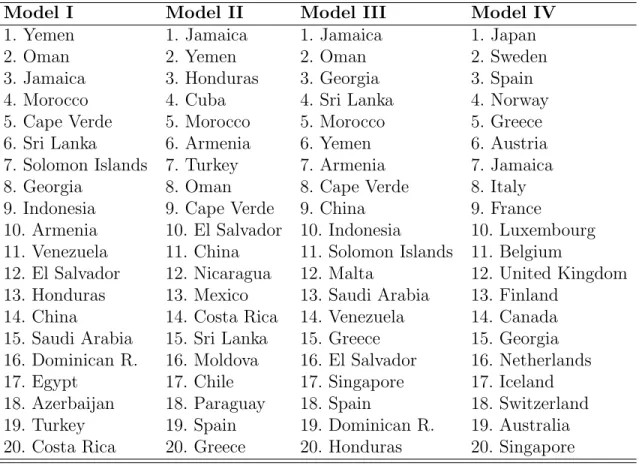
In order to observe in detail the changes that occur in the top ranked countries under the different models, Table III shows the top 20 most efficient countries under all four models. Although there are differences, the ranking is quite stable when we consider the first three models. All of these include countries from Middle East, Asia, North of Africa and Latin America. However, this changes completely when observed heterogeneity affects the scale of inefficiencies. In Model IV, the developed countries rank in the first positions as might be intuitively expected. For example, Japan, Sweden and Norway are the top 3 countries under this model while they are ranked 30, 55 and 58 under the base model. The opposite is also observed for some developing countries which are surprisingly very efficient when heterogeneity is not considered such as Yemen and Cape Verde, among others.
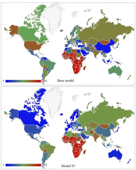
Changing the scale of the inefficiency through observed covariates has an effect over the rankings and this is illustrated in Figure 3. While most of the African countries continue to show low efficiency; there is a significant change in the classification of the top and middle ranked observations. The best performing countries, in particular, the developed countries are very
Table III
Top 20 most efficient countries
Model I Model II Model III Model IV 1. Yemen 1. Jamaica 1. Jamaica 1. Japan 2. Oman 2. Yemen 2. Oman 2. Sweden 3. Jamaica 3. Honduras 3. Georgia 3. Spain 4. Morocco 4. Cuba 4. Sri Lanka 4. Norway 5. Cape Verde 5. Morocco 5. Morocco 5. Greece 6. Sri Lanka 6. Armenia 6. Yemen 6. Austria 7. Solomon Islands 7. Turkey 7. Armenia 7. Jamaica 8. Georgia 8. Oman 8. Cape Verde 8. Italy 9. Indonesia 9. Cape Verde 9. China 9. France
10. Armenia 10. El Salvador 10. Indonesia 10. Luxembourg 11. Venezuela 11. China 11. Solomon Islands 11. Belgium
12. El Salvador 12. Nicaragua 12. Malta 12. United Kingdom 13. Honduras 13. Mexico 13. Saudi Arabia 13. Finland
14. China 14. Costa Rica 14. Venezuela 14. Canada 15. Saudi Arabia 15. Sri Lanka 15. Greece 15. Georgia 16. Dominican R. 16. Moldova 16. El Salvador 16. Netherlands 17. Egypt 17. Chile 17. Singapore 17. Iceland 18. Azerbaijan 18. Paraguay 18. Spain 18. Switzerland 19. Turkey 19. Spain 19. Dominican R. 19. Australia 20. Costa Rica 20. Greece 20. Honduras 20. Singapore
sensitive to the inclusion of relevant covariates such as income and inequality that distinguish them from developing countries.
The difference in the rankings obtained with Model IV is justified by significant moves and shrinkages of the individual posterior efficiency distributions. Figure 4 shows the posterior 90% credible intervals of efficiencies for some selected countries. It can be seen that the intervals are narrower when the observed heterogeneity affects the scale of the inefficiency since the estimations uncertainty diminishes. Moreover, the gap between the worst and the best performing countries increases under Model IV, resulting in less overlaps of the posterior distributions. Countries with the lowest indicators on the heterogeneity variables such as the African countries obtain even lower scores, while developed countries improve. The case of US is remarkable, it occupies position 45 under Model IV, while it ranks 140 under the base model. Less dispersion and overlaps of the posterior efficiency distributions allow for more reliable conclusions about the
Base model
Model IV
Figure 3. Countries’ efficiency rankings by color rankings obtained.
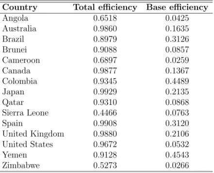
As mentioned previously, one of the advantages of preserving the scaling property is the de-composition of the one-sided error term into a base and a heterogeneity component. In particular, considering half-normal distributed inefficiencies, uit = |Uit∗| · exp(hi, γ) where Uit∗ ∼ N (0, σU2).
Table IV presents this decomposition in terms of efficiency for the selected countries in Figure 4. We observe that countries such as Yemen, Brazil and Colombia present higher base efficiency but lower total efficiency than developed countries. This may indicate that these countries present good managerial skills in health provision but under their specific characteristics, they exploit
0.4 0.5 0.6 0.7 0.8 0.9 1 Zimbabwe Yemen United States United Kingdom Spain Sierra Leone Qatar Japan Colombia Canada Cameroon Brunei Brazil Australia Angola Model I Model II Model III Model IV
Figure 4. 90% credible intervals of the posterior efficiency distributions for selected countries with half-normal inefficiencies
their management abilities to a lesser extent than the developed countries. One of the countries taking great advantage of environmental characteristics is the USA, whose efficiency in health provision seems to be almost totally dependent in their particular attributes. These results are in line with those obtained by contrasting the base model and Model IV. Other group of coun-tries, mainly from Africa exhibit low base and low total efficiency. This may indicate both, poor natural managerial abilities, and inability to perform well under their relative bad conditions. This may explain why these countries present very bad performance under all models whether heterogeneity is considered or not.
Overall, we observe that allowing heterogeneity to change the scale but not the shape of inef-ficiency distributions has relevant effects on shrinking and moving the distributions of posterior individual efficiencies. The covariates are found to be inefficiency related and their inclusion affecting the scale of the one sided error component distribution has a large impact on the coun-tries’ efficiency ranking. This may change the conclusions derived from the study and have possible implications over health policies.
Table IV
Efficiency decomposition for selected countries Country Total efficiency Base efficiency
Angola 0.6518 0.0425 Australia 0.9860 0.1635 Brazil 0.8979 0.3126 Brunei 0.9088 0.0857 Cameroon 0.6897 0.0259 Canada 0.9877 0.1367 Colombia 0.9345 0.4489 Japan 0.9929 0.2135 Qatar 0.9310 0.0868 Sierra Leone 0.4466 0.0763 Spain 0.9908 0.3120 United Kingdom 0.9880 0.2106 United States 0.9672 0.0532 Yemen 0.9128 0.4543 Zimbabwe 0.5273 0.0266
B. Application to Airlines
The airline industry is an interesting sector where performance and efficiency have been studied in the literature through parametric and non-parametric methods. Usually, production functions are employed to evaluate technical efficiency and environmental covariates are often included in the frontier as exogenous variables (see Coelli et al., 1999).
In this application we use a Cobb-Douglas cost function with an output quadratic term to evaluate economic efficiency of the airline industry. The model in (6) can be easily extended to a cost function and as in the previous application we consider individual characteristics to capture firms heterogeneity. We use a data set of 24 US domestic airlines over 15 years, from 1970 to 1984, with a total of 246 observations. This is a revised sample obtained from a data set used by Greene (2008).5
We estimate four stochastic frontier models similar to those proposed in the previous ap-plication. For each model the inefficiency component is assumed to follow: a) half-normal, b)
5The original data set includes 256 observations, ten years of observations for an extra airline company. We
truncated normal, or c) exponential distributions. We impose regularity conditions on prices and output in order to accomplish positive elasticities. The general specification that encompasses our four models is the following:
ln Cit= α + β1ln P mit+ β2ln P fit+ β3ln P lit+ β4ln P eit
+ β5ln(yit) + β612ln2(yit) + β7t + β8t2 + hitδ + vit+ uit
vit ∼ N (0, σv2); uit= |Uit|
a) Uit ∼ N (0, σ2U it· (exp(hitγI1+ τitI2))2)
b) Uit ∼ N (µ · exp(hitγI1+ τitI2), σU it2 · (exp(hitγI1+ τitI2))2)
c) Uit ∼ exp(λit· exp(hitγI1+ τitI2)),
(8)
where Cit is the total cost supported by airline i at time t in the output production, and P mit,
P fit, P lit, P eit are the input prices of material, fuel, labor and equipment, respectively. Cost
and prices are normalized by the property price. yit is the output of airline i at time t and it is
an index that aggregates regular passenger, mail, charter, and other freight services. With the purpose to capture possible technological changes over the 15 years covered by the sample we include a trend and its square into the model.
Regarding heterogeneity, the vector of observed covariates is hit = [Loadit, Stageit, P ointsit],
and τit is the unobserved heterogeneity unknown parameter. Variables in hit are load factor,
average stage length and points served. Load factor is the effective performed tonne-passenger per kilometer by the airline as a proportion of the total available tonne-passenger per kilometer. This is a capital utilization ratio which can be seen as a measure of either demand or operational optimization. Stage length is the ratio of total performed kilometers to the total number of departures. It defines whether or not the airline makes long or short flights and measures scale effects. Finally, the number of points served is a measure of network size and its effects.6
The base model (Model I) does not consider any type of heterogeneity; therefore, δ = 0, γ = 0 and I1 = I2 = 0. The last two assumptions apply for Model II, which considers only
6The first two covariates are commonly used in productivity and efficiency applications as well as other variables
technological heterogeneity by including hit in the cost function. As in the WHO application,
Model III accounts only for unobserved inefficiency heterogeneity through τit. Also, it is possible
to think of covariates in hit to be related with inefficiencies in the sense that the length of flights
may have an effect on the unproductive time of aircrafts; different utilizations of the aircrafts may imply different fix costs sharing; and, the network size may affect coordination and routes optimization. Therefore, Model IV considers the scale of the non-negative error component to be affected by these observed covariates.7
Table V
Model comparison criteria assuming different distributions for the inefficiency Distribution Model I Model II Model III Model IV Model V Half normal DIC -332.6250 -479.2080 -350.2240 -374.8520 -485.1709 LPS -32.1260 -77.6020 -40.1970 -52.5360 -78.5218 MSE 0.0264 0.0093 0.0259 0.0172 0.0112 Truncated normal DIC -403.6720 -606.3150 -413.9810 -525.8170 -614.7094 LPS -13.7340 -33.6520 -15.3840 -21.6690 -33.6910 MSE 0.0257 0.0096 0.0255 0.0178 0.0093 Exponential DIC -309.3740 -455.6980 -317.1460 -353.3810 -453.8130 LPS -1.5550 -11.6580 -2.1830 -9.5760 -11.6927 MSE 0.0318 0.0207 0.0297 0.0238 0.0214
From Table V we observe that the results are robust, both in terms of fit and predictive performance, to the inefficiency component distributions. Models that include either observed or unobserved heterogeneity present better values for the DIC, LPS and MSE than those obtained with the base models. Moreover, the best performance is exhibited by models that include exogenous variables in the cost function. Therefore, we conclude that load factor, stage length and the number of served points are more likely to be technological related than inefficiency related factors. This leads us to propose an extra model (Model V) that includes the observed covariates in the frontier but also accounts for unobserved heterogeneity in the inefficiency. This model presents improvements in most of the performance indicators across distributions.
7We considered a fifth model that included both observed and unobserved heterogeneity in the sale parameter
of inefficiency, but the results were roughly the same than those obtained in Model IV. As in the WHO application, this could mean that the covariates used capture all relevant heterogeneity in the inefficiency.
These results differ from those obtained by Greene (2008), where no differences were reported when heterogeneity variables were included in the mean of a truncated inefficiency component compared to a model with the covariates in the cost function. This could be due to the fact that we include the covariates in a way that they affect the scale but not the shape of the inefficiency distribution. Also, we impose regularity conditions in prices, which lead our models to present the expected coefficient signs.8
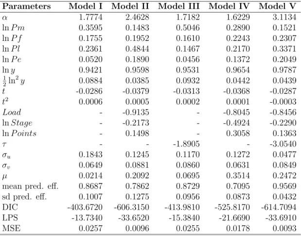
Regarding distributions, it is not possible to identify which one leads the different models to perform the best. In general, models with inefficiency component following a half-normal distri-bution exhibit the best LPS and models with truncated normal distributed inefficiencies present the best DIC. However, as in the WHO application, rankings are almost unaltered across distri-butions. So, hereafter, we report results with truncated normal inefficiencies. Table VI reports the posterior means of the parameter distributions. We can observe that the inclusion of either unobserved or observed heterogeneity that affects the scale but not the shape of the inefficiencies diminishes the predictive efficiency dispersion and moves its mean toward 1. Regarding the coef-ficients, we can check that increasing the aircraft utilization and the flights length have negative effects in costs and inefficiency, while a larger network has the opposite effect. Interpretations of the effect of covariates over inefficiency can be done in the same way as in the WHO case given the scaling property.
Including any type of heterogeneity change, the estimations of posterior mean efficiencies with respect to the base model as we observe in Figure 5. Also choosing where to include covariates is important. Figure 6 shows that mean efficiencies are very different if we include them in the cost function or in the inefficiency parameters. Moreover, if covariates are found to be technological related as in this case, we still can model unobserved effects on the inefficiency. In fact, including unobserved heterogeneity in Model V has important effects on shrinking and moving the posterior efficiencies compared to Model II. In Figure 6, we observe that posterior mean efficiencies move close to the frontier for most of observations. This may indicate that the unobserved component
Table VI
Posterior means of the parameter distributions with truncated normal distributed inefficiencies
Parameters Model I Model II Model III Model IV Model V α 1.7774 2.4628 1.7182 1.6229 3.1134 ln P m 0.3595 0.1483 0.5046 0.2890 0.1521 ln P f 0.1755 0.1952 0.1610 0.2243 0.2307 ln P l 0.2361 0.4844 0.1467 0.2170 0.3371 ln P e 0.0520 0.1890 0.0456 0.1372 0.2049 ln y 0.9421 0.9598 0.9531 0.9654 0.9787 1 2ln 2y 0.0884 0.0385 0.0932 0.0442 0.0439 t -0.0286 -0.0379 -0.0313 -0.0368 -0.0287 t2 0.0006 0.0005 0.0002 0.0001 -0.0003 Load - -0.9135 - -0.8045 -0.8456 ln Stage - -0.2173 - -0.4924 -0.2290 ln P oints - 0.1498 - 0.3058 0.1363 τ - - -1.8905 - -3.0540 σu 0.1843 0.1245 0.1170 0.1272 0.0477 σv 0.0649 0.0881 0.0860 0.0631 0.0849 µ 0.0214 0.2092 0.0695 0.3514 0.2472 mean pred. eff. 0.8687 0.7862 0.8729 0.7095 0.9569 sd pred. eff. 0.1007 0.1275 0.0956 0.0873 0.0432 DIC -403.6720 -606.3150 -413.9810 -525.8170 -614.7094 LPS -13.7340 -33.6520 -15.3840 -21.6690 -33.6910 MSE 0.0257 0.0096 0.0255 0.0178 0.0093
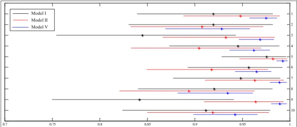
captures some factors that were attributed to inefficiency under Model II. However, their relative positions are preserved and the effect on rankings is very little. At an individual level, Figure 7 shows 90% posterior credible intervals for posterior efficiencies for 10 selected airlines in their last observed year. We can see a strong shrinkage effect on these intervals when we take into account the unobserved heterogeneity in the inefficiency that preserves the scaling property.
Preserving the scaling property makes individual inefficiency decomposition possible. In this case, for the truncated normal inefficiency: uit = |Uit∗| · exp(τit) where Uit∗ ∼ N (µ, σU2).
Table VII presents this decomposition in terms of efficiency for Model V and for the 10 selected airlines plotted in Figure 7. Although there are small differences in the total efficiency among airlines, when it is decomposed we observe large differences in their natural managerial skills. The difference between the base and total efficiency allows us to distinguish the way unobserved firm
Figure 5. Mean efficiencies under truncated normal distribution - Base model vs. heterogeneity models
Figure 6. Mean efficiencies under truncated normal distribution - Model II vs. Model IV and Model V
effects are handled by airlines managers. For instance, airline 12 presents lower base efficiency but higher total efficiency than airline 17, suggesting that the former handles better their specific characteristics.
Summing up, performance indicators suggest that firm characteristics such as the distance among destinations, the capacity offered, and the size of the network differentiates the airlines in terms of technology (e.g. type of aircraft). However, dispersion of individual posterior efficiencies is the lowest when exogenous variables are included in the inefficiency component when the scaling property is preserved. This holds when observed covariates are technological and unobserved heterogeneity in the inefficiency is added.
0.7 0.75 0.8 0.85 0.9 0.95 1 1 2 3 4 5 6 7 8 9 10 Model I Model II Model V
Figure 7. 90% credible intervals of the posterior efficiency distributions for selected airlines with truncated normal inefficiencies
Table VII
Efficiency decomposition for selected airlines Airline ID Total efficiency Base efficiency
1 0.9651 0.4568 2 0.9411 0.2822 5 0.9562 0.3888 7 0.9488 0.3499 8 0.9803 0.6404 9 0.9527 0.3641 12 0.9713 0.3211 17 0.9472 0.5270 18 0.9728 0.5505 19 0.9537 0.3707
V. Conclusions and Extensions
In stochastic frontier analysis the inefficiency component may be erroneously estimated when firm characteristics are not taken into account. These firm characteristics induce heterogeneity that might result in different firm frontiers, or may have an impact directly on the inefficiencies. In this work we put forward the modeling of heterogeneity in a Bayesian context by capturing both the observed and unobserved heterogeneity in the inefficiency component distribution. Firm characteristics are included through either exogenous variables or a random parameter which are allowed to be time-varying and such that the scale but not the shape of the inefficiency is
altered. The inefficiencies are assumed to follow half-normal, truncated normal and exponential distributions that preserves this property. Finally, the models were fitted to two, well known, data sets previously studied only in the frequentist context. The WinBugs package was used to implement the Bayesian inference. Results were compared to those obtained with frontier models that ignore heterogeneity or include heterogeneity just in the frontier.
Our findings suggest that considering firms’ heterogeneity that have effects on the scale but not in the shape of inefficiencies leads the models to improve in terms of goodness of fit and predictive performance, and has a shrinkage effect that reduces the uncertainty on mean scores and rankings. The inclusion of unobserved heterogeneity in the inefficiency is also found to be relevant when exogenous variables are not available or when they are found to be technology related and consequently, should be more investigated. Regarding this issue, we propose a very intuitive procedure by including a random parameter in the parameters of the inefficiency component distribution.
A future research possibility is the study of different specifications to capture unobserved effects in the inefficiency, as well as, the use of different distributions. A second area is the inclusion of dynamic effects in the inefficiency specification, see e.g. Tsionas (2006). Work is currently in progress on these areas.
References
Aigner, D., C. Lovell, and P. Schmidt (1977). Formulation and estimation of stochastic frontier production function models. Journal of Econometrics 6, 21–37.
Alvarez, A., C. Amsler, L. Orea, and P. Schmidt (2006). Interpreting and testing the scaling property in models where inefficiency depends on firm characteristics. Journal of Productivity Analysis 25, 201–212.
Battese, G. E. and T. Coelli (1995). A model for technical inefficiency effects in a stochastic frontier production model for panel data. Empirical Economics 20, 325332.
Caudill, S. and J. Ford (1993). Biases in frontier estimation due to heteroscedasticity. Economics Letters 41, 17–20.
Caudill, S., J. Ford, and D. Gropper (1995). Frontier estimation and firm-specific inefficiency measures in the presence of heteroskedasticity. Journal of Business and Economics Statis-tics 13, 105–111.
Coelli, T., S. Perelman, and E. Romano (1999). Accounting for environmental influences in stochastic frontier models: With application to international airlines. Journal of Productivity Analysis 11, 251–273.
Ferreira, J. and M. Steel (2007). Model comparison of coordinate-free multivariate skewed dis-tributions with an application to stochastic frontiers. Journal of Econometrics 137, 641–673. Good, I. (1952). Rational decisions. Journal of the Royal Statistical Society B 14, 107–114. Greene, W. (1990). A gamma-distributed stochastic frontier model. Journal of Econometrics 46,
141–164.
Greene, W. (2004). Distinguishing between heterogeneity and inefficiency: Stochastic frontier analysis of the World Health Organization’s panel data on national health care systems. Health Economics 13, 959–980.
Greene, W. (2005). Reconsidering heterogeneity in panel data estimators of the stochastic frontier model. Journal of Econometrics 126, 269–303.
Greene, W. (2008). The Econometric Approach to Efficiency Analysis. The Measurement of Productive Efficiency and Productivity Growth, Chapter 2, pp. 959–980. Oxford University Press, Inc.
Griffin, J. and M. Steel (2004). Semiparametric Bayesian inference for stochastic frontier models. Journal of Econometrics 123, 121–152.
Griffin, J. and M. Steel (2007). Bayesian stochastic frontier analysis using WinBUGS. Journal of Productivity Analysis 27, 163–176.
Griffin, J. and M. Steel (2008). Flexible mixture modelling of stochastic frontiers. Journal of Productivity Analysis 29, 33–50.
Hadri, K. (1999). Estimation of a doubly heteroscedastic stochastic frontier cost function. Journal of Productivity Analysis 17, 359–363.
Huang, H. (2004). Estimation of technical inefficiencies with heterogeneous technologies. Journal of Productivity Analysis 21, 277–296.
Huang, H. and J. Liu (1994). Estimation of a non-neutral stochastic frontier production function. Journal of Productivity Analysis 5, 171180.
Koop, G., J. Osiewalski, and M. Steel (1997). Bayesian efficiency analysis through individual effects: Hospital cost frontiers. Journal of Econometrics 76, 77–106.
Koop, G., M. Steel, and J. Osiewalski (1995). Posterior analysis of stochastic frontier models using Gibbs sampling. Comput Stat 10, 353–373.
Kumbhakar, S., S. Ghosh, and J. J. McGuckin (1991). A generalized production frontier ap-proach for estimating determinants of inefficiency in U.S. dairy farms. Journal of Business and Economic Statistics 9, 279286.
Kumbhakar, S. and K. Lovell (2000). Stochastic Frontier Analysis. New York: Cambridge University Press.
Meeusen, W. and J. van den Broeck (1977). Efficiency estimation from Cobb-Douglas production functions with composed errors. International Economic Review 8, 435–444.
Reifschnieder, D. and R. Stevenson (1991). Systematic departures from the frontier: A framework for the analysis of firm inefficiency. International Economic Review 32, 715723.
Simar, L., K. Lovell, and P. van den Eeckaut (1994). Stochastic frontiers incorporating exogenous influences on efficiency. Discussion paper no. 9403, Institut de Statistique, Universit Catholique de Louvain.
Spiegelhalter, D., N. Best, B. Carlin, and A. Van der Linde (2002). Bayesian measures of model complexity and fit. Journal of the Royal Statistical Society 64 (4), 583–616.
Stevenson, R. (1980). Likelihood functions for generalized stochastic frontier estimation. Journal of Econometrics 13, 57–66.
Tandon, A., C. Murray, J. Lauer, and D. Evans (2000). Measuring overall health system perfor-mance for 191 countries. GPE Discussion Paper Series 30.
Tsionas, E. (2002). Stochastic frontier models with random coefficients. Journal of Applied Econometrics 17, 127–147.
Tsionas, E. (2006). Inference in dynamic stochastic frontier models. Journal of Applied Econo-metrics 21, 669–676.
van den Broeck, J., G. Koop, J. Osiewalski, and S. MFJ (1994). Stochastic frontier models: A Bayesian perspective. Journal of Econometrics 61, 273–303.
Wang, H. (2002). Heteroscedasticity and non-monotonic efficiency effects of a stochastic frontier model. Journal of Productivity Analysis 18, 241–253.
Wang, H. and P. Schmidt (2002). One step and two step estimation of the effects of exogenous variables on technical efficiency levels. Journal of Productivity Analysis 18, 129–144.
WHO (2000). Health Systems: Improving Performance. The World Health Report. Geneva: World Health Organization.