A Work Project, presented as part of the requirements for the Award of a Master Degree in Economics from the NOVA – School of Business and Economics and INSPER.
ANALYSIS OF THE BRAZILIAN YIELD CURVE: A NO-ARBITRAGE FACTOR-AUGMENTED VECTOR AUTOREGRESSION APPROACH
BRUNO LUIZ DE MIRANDA SANTOS - 887
A Project carried out on the Master in Economics Program, under the supervision of: Professor. Dr. Ricardo Brito / INSPER and Professor Dr. André Silva / Universidade Nova de Lisboa
Abstract
This dissertation: ANALYSIS OF THE BRAZILIAN YIELD CURVE: A NO-ARBITRAGE FACTOR-AUGMENTED VECTOR AUTOREGRESSION APPROACH, applies a parsimonious method to analyse the Brazilian term structure exploiting a vast number of macroeconomic variables. The procedure, developed in Moench (2008), combines the short-term interest rate with the principal components extracted from a large macroeconomic dataset. The short-term dynamics are described by a factor-augmented vector autoregression. Subsequently, the term structure is obtained by the no-arbitrage method. The results in-sample and out-of-sample of the so called No-arbitrage Factor Augmented Vector Autoregression (NAFAVAR) model is compared with the model in Diebold and Li (2006), since this model delivers both in-sample fitting and out-of-sample forecasts. The results of the NAFAVAR model outperforms the competitor model in some maturities of the term structure, which could be helpful for out-of-sample forecasts. The NA-FAVAR model seems to adapt well to the Brazilian interest rate market, which could help financial agents to evaluate and forecast securities using a model with macroeconomic interpretation.
Keywords: Factors, VAR, Interest Rates, No-Arbitrage Models.
JEL Codes: C38, E43, E44, E47. 1. Introduction
Latent-factor models are largely accepted to describe and forecast interest rates. Nelson and Siegel (1987), Svensson (1994) and Vasicek (1977), for instance, use the traditional method of decomposing yields into latent factors in order to deliver an in-sample fit to the observable data. Other models are used to forecast out-of-sample interest rates, such as those mentioned by Duffee
(2002) and Diebold and Li (2006). Generally, it is accepted that three factors describe practically the whole amount of the interest rates’ variation, named as level, slope and curvature, depending on which features of the term structure they affect. Unfortunately, those models do not provide any economic explanation of the yield curve dynamics. Moench (2008) uses a procedure that not only generates better forecast results but also provides economic interpretations.
Ang and Piazessi (2003) combine the traditional latent factor model with two macroeconomic components using a Taylor-rule approach. Their results show that the economic factors explain a considerable part of the interest rates’ variation, resulting in an improvement in the forecast outcomes. Although there were developments in the latent-economic-factors based models throughout the following years, it was only with Bernanke and Boivin (2005) that the term structure was modeled in a “data-rich environment” approach, based on the fact that central banks use a large amount of economic information to set a course of action through monetary policies. In this regard, Bernanke and Boivin suggest that common factors could be extracted from a large number of macroeconomic time series to explain the term structure dynamics of interest rates throughout a structural vector autoregression analysis.
Moench (2008) added no-arbitrage restrictions to the Bernanke (2005) model in order to extrapolate the short-term dynamics to the entire yield curve. He structured his model using a Factor Augmented Vector Autoregression (FAVAR) to depict the fundamental features of short-term yield through factors extracted from large datasets of macroeconomic variables and then derive the whole term structure imposing no-arbitrage restrictions on the parameters. The first step is the extraction of common factors of the macroeconomic dataset using Stock and Watson (2002a,b) approach. This methodology consists of modelling the covariability of the macroeconomic time series in terms of some unobserved latent factors using the principal
component approach. Second, a no-arbitrage VAR of interest rates on the factor is implemented. The development of the NAFAVAR could increase the capability of the different market agents in understanding the relationship between interest rates and macroeconomic variables. The better forecast of the results could also improve the valuation of several market securities, such as options and other derivatives, equities and interest rate related financial instruments.
In this dissertation, the objective is to apply the no-arbitrage factor augmented vector autoregression approach, suggested by Moench (2008), for the Brazilian financial market in order to predict the term structure of interest rate and compare its results with the traditional latent model forecasts.
The results show that the NAFAVAR model outperformed the competitor’s model (Diebold-Li Model) by almost half of the model’s RMSE (Root Mean Square Error) in the out-of-sample forecast for six and twelve months ahead. Although the Diebold-Li model provides a better in-sample fit, the NAFAVAR model provides a suitable fit and macroeconomic interpretations of the results.
This dissertation is structured as follows: Section 2 describes the data selected for this research; Section 3 shows the no-arbitrage factor augmented VAR model and its specifications; Section 4 presents the in-sample results of the models; In section 5, the model is applied in out-of-sample estimations; and Section 6 concludes.
2. Dataset
In order to estimate factors which could summarize the cross-sectional dynamics of the Brazilian economy, several economic time series were gathered. In total, 161 monthly time series compose the panel data. The study comprises the period from January 2003 to May 2016. The series were
classified as follows: real output, income, employment rates, working hours, consumption, stock prices, exchange rates, money quantity, credit quantity aggregates, price indexes, average hourly earnings and miscellaneous. The series used to estimate the NA-FAVAR in the Brazilian economy were taken from Banco Central do Brasil, IBGE, IPEA Data, FGV, and several other institutions. The stationarity of each time series were assessed by Dickey-Fuller Stationarity Test followed by the necessary transformations in order to respect the no-unitary root rule. As transformation, it was utilised the first difference, logarithmic difference, logarithmic conversion, and logarithmic conversion of the division between two consecutive periods of the time series.
The Brazilian interest rate term structure is analysed using zero coupon bond yields with maturities of 1, 2, 3, 4, 5, 6, 7, 8, 9, 11, 12, 24, 36 and 60 months. The interest rates are continuously-compounded and have been gathered from the Brazilian Central Bank (Banco Central do Brasil). All time series are standardized in order to have mean zero and unit variance.
3. Model
The intention of this analysis is to follow as strictly as possible the procedure developed in Moench (2008). The NAFAVAR model is estimated in two steps. First, the common factors are calculated using Stock and Watson (2002 a, b) approach. Subsequently, we add the one-month interest rate in order to derive the joint dynamics. Here, the interest rate is assumed to be unconditionally orthogonal to all the factors. The factors are ordered by the size of their eigenvalues (extracted from the variance-covariance matrix of the dataset). The quantity of factor was selected using two criteria: 1. parsimony; and 2. as much factors as necessary to explain more than 99.9% of the variance of the entire dataset. This criteria gives 4 factors as the enough quantity. Going further, the Hannan-Quinn information criterion is applied to obtain the optimum number of lags for the
VAR on factors and interest rate reaching 4 lags as optimum. Secondly, we estimate a VAR of the interest rate yields on the common factors and the one-month interest rates in order to derive the price of risk parameters following Ang (2006) approach.
The FAVAR model summarises information from a large number of time series into non-observable variables or factors (variables not directly observed but rather inferred), which could be interpreted as a diffuse concept, such as “economic activity” or “credit conditions”. The factors are forces that affect cross-sectionally the entire economy.
The common factors extraction formulation could be summarised as follows:
𝑋𝑡= Λ𝐹𝐹𝑡+ Λ𝑟𝑟𝑡+ 𝑒𝑡 (1) (𝐹𝑡 𝑟𝑡) = 𝜇 + Φ(𝐿) ( 𝐹𝑡−1 𝑟𝑡−1) + 𝜔𝑡 (2) where,
𝑋𝑡 is the observable macroeconomic variables vector (Mx1)of period t, with T observations Λ𝐹 𝑎𝑛𝑑 Λ𝑟are factor loading matrices (Mxk)and (Mx1)
𝐹𝑡 𝑖𝑠 𝑡ℎ𝑒 vector of the factors (kx1) 𝑟𝑡 is the one month interest rate
𝑒𝑡 is the idiosyncratic components vector(Mx1) 𝜇 is the vector of constant(k + 1x1)
𝜔𝑡is the vector of reduced form shocks with var − covar matrix Ω
𝑍𝑡= 𝝁 + 𝚽𝑍𝑡−1+ 𝝎𝑡 (3)
where,
𝑍𝑡 = (𝐹𝑡´, 𝑟𝑡, 𝐹𝑡−1´ , 𝑟𝑡−1, … , 𝐹𝑡−𝑝+1´ , 𝑟𝑡−𝑝+1)
𝑟𝑡= 𝛿´𝑍 𝑡
and 𝝁, 𝚽, 𝝎𝒕 , 𝛀 denote the companion form equivalents of 𝜇, Φ, 𝜔𝑡 , Ω.
To make the FAVAR in (3) be in accordance with the no-arbitrage assumption the martingale dynamics is introduced, as follows:
𝑀𝑡+1 = exp(−𝛿𝑡´𝑍
𝑡− 1/2𝜆𝑡´𝛀𝜆𝑡− 𝜆𝑡´𝝎𝑡+1) (4)
where 𝜆𝑡 is the market price of risk and its dynamics can be derived as follows:
𝜆𝑡 = 𝜆0+ 𝜆1𝑍𝑡 (5)
It is possible to see that 𝜆𝑡 is dependent only on contemporaneous observations of the factors.
The following equation guarantees the no-arbitrage assumption:
𝑃𝑡(𝑛) = 𝐸𝑡(𝑀𝑡+1𝑃𝑡+1(𝑛−1)) ⇒ 𝑃𝑡(𝑛) = exp (𝐴𝑛+ 𝐵𝑛´𝑍𝑡)
where n is the maturity of the bond and A and B are derived as follows:
𝐴𝑛 = 𝐴𝑛−1+ 𝐵𝑛−1(𝝁 + 𝛀𝜆0) + 1/2𝐵𝑛−1´ 𝛀𝐵𝑛−1 (6)
𝐵𝑛´ = 𝐵𝑛−1´ (𝚽 − 𝛀𝜆1) − 𝛿´ (7)
When calculating 𝐴1 and 𝐵1, it is easy to see that 𝐴0 = 0 and 𝐵0 = −𝛿´. Further maturities follow
Finally, once the yields are affine in the state variables, the yield is obtained by the following equation:
𝑦𝑡(𝑛)= −(1/𝑛)𝐴𝑛− (1/𝑛)𝐵𝑛´𝑍𝑡 (8)
The model is entirely defined by equations (1), (3), (6), (7) and (8).
The extraction method implied in equation (1), suggested by Stock and Watson (2002a,b), is described below.
Let 𝐹̂ and 𝛬̂ be the estimate of the factors and the factor loadings, respectively, and derived as follows:
𝐹̂ = √𝑇𝑉
Λ̂ = √𝑇𝑋′𝑉
where V denotes the eigenvectors corresponding to the k largest eigenvalues of the TxT variance-covariance matrix XX´ of the macro dataset, subjected to normalisation (F´F/T=Ik).
Once r is observable, it is important to guarantee the unconditionally orthogonality between r and the unobserved factors F. Moench (2008) isolates it from the latent factors F by regressing the macro variables onto r and getting the principal components from the residuals of each regression. The number of factors is fixed due to limited computational constraints created by the market prices of risk and the parsimonious criteria.
After the principal component estimation, the companion form equivalent of the parameters , , and also 𝝎𝒕 are calculated by a VAR with four lags on the short-term interest rate.
of squared fitting errors of the model following the nonlinear least square approach proposed by Ang et al. (2006) in order to describe the dynamics of the evolution of the state prices of risk, what is done by minimising the following equation on the parameters 𝜆0 and 𝜆1:
𝑆 = ∑𝑇𝑡=1∑𝑁𝑛=1(𝑦̂𝑡(𝑛)− 𝑦𝑡(𝑛))2 (9)
where:
𝑦̂𝑡(𝑛) = 𝑎̂𝑛 + 𝑏̂𝑛´𝑍𝑡
It is assumed that the market prices of risk are affected only by contemporaneous factors observations. In that way, the parameters 𝜆0 and 𝜆1 are set as follows:
𝜆0 = (𝜆̃0´´, 01𝑥(𝑘+1)(𝑝−1)) ´
𝜆1 = ( 𝜆̃1 0(𝑘+1)𝑥(𝑘+1)(𝑝−1)
0(𝑘+1)(𝑝−1)𝑥(𝑘+1) 0(𝑘+1)(𝑝−1)𝑥(𝑘+1)(𝑝−1)
)
where 𝜆̃0 𝑖𝑠 𝑎 (𝑘 + 1) matrix and 𝜆̃1 𝑖𝑠 𝑎 (𝑘 + 1)𝑥(𝑘 + 1) matrix.
The parameters 𝜆0 and 𝜆1are initially set as constant-non-zeros and zeros, respectively.
4. Empirical Results
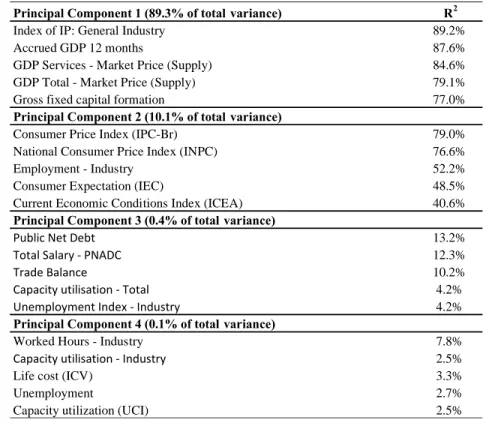
After performing the first step, which comprises the extraction of the common components of the economic dataset, we determine the percentage of the variation of all time series which could be explained by the factors. Table 1 shows the amount of the variance of the whole dataset explained by the four factors with the largest eigenvalues. The first factor alone explains 89.3% of the entire panel’s variance while, in Moench (2008), the first factor explains only 25.10% of the variance of all USA macroeconomic variables present in the dataset.
Table 1 analyses the correlation between the factors and variables which are commonly regarded as important instruments to describe the interest rate dynamics, such as, GDP, unemployment and inflation rate. In table 1, also, shows the percentage of the variance of the entire dataset explained by each of the four factors. Due to identification restrictions (non-singular rotation), the factors do not present a structural economic interpretation, but Bernanke et al. (2003) interprets them as diffuse concepts, such as “economic activity” or “credit conditions”, which could not be described by a small number of series, but are rather implicit in a large economic dataset.
Table 1 - Share of variance explained by factors
Principal Component 1 (89.3% of total variance) R2
Index of IP: General Industry 89.2%
Accrued GDP 12 months 87.6%
GDP Services - Market Price (Supply) 84.6%
GDP Total - Market Price (Supply) 79.1%
Gross fixed capital formation 77.0%
Principal Component 2 (10.1% of total variance)
Consumer Price Index (IPC-Br) 79.0%
National Consumer Price Index (INPC) 76.6%
Employment - Industry 52.2%
Consumer Expectation (IEC) 48.5%
Current Economic Conditions Index (ICEA) 40.6%
Principal Component 3 (0.4% of total variance)
Public Net Debt 13.2%
Total Salary - PNADC 12.3%
Trade Balance 10.2%
Capacity utilisation - Total 4.2%
Unemployment Index - Industry 4.2%
Principal Component 4 (0.1% of total variance)
Worked Hours - Industry 7.8%
Capacity utilisation - Industry 2.5%
Life cost (ICV) 3.3%
Unemployment 2.7%
Capacity utilization (UCI) 2.5%
We regress the yields on factors and also on output and inflation rate in order to have preliminary indications of the explanatory capacity of the factors as exogenous variables to estimate the interest rates. These tests attempt clarify whether the factors regression on interest rates generates better explanations than a commonly known Taylor-rule model of inflation and output. These regressions follow Davidson and MacKinnon (1993) approach. Afterwards, it was performed unrestricted
regressions of the interest rates on the common factors.
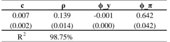
Table 2 - Policy rule based on individual variables
c ρ ϕ_y ϕ_π
0.007 0.139 -0.001 0.642
(0.002) (0.014) (0.000) (0.042)
R2 98.75%
Table 2 shows the parameters in the first line, the standard errors in the second line and the adjusted R2 of the regression of a policy rule based on inflation and output with partial adjustments based
on one-month lag of the interest rate analysed, following the equation bellow: 𝑟𝑡 = 𝑐 + 𝜌𝑟𝑡−1+ (1 − 𝜌)(𝜙𝑦𝑦𝑡+ 𝜙𝜋𝜋𝑡) + 𝑒𝑡
where 𝑦 denotes the GDP and 𝜋 the annual rate of inflation measured as of IPCAs inflation index, the period analysed comprises data from January 2003 to May 2006.
Table 3 - Policy rule based on factors
c ϕ_r ϕ_F1 ϕ_F2 ϕ_F3 ϕ_F4
0.0015 0.9868 0.0005 -0.0015 -0.0002 0.0236 (0.0013) (0.0104) (0.0003) (0.0008) (0.0032) (0.0107)
R2 99.50%
Table 3 shows in the first line the parameters, the standard errors in the second line, and the adjusted R2 of the regression of a policy rule based on the four factors extracted from the dataset
with partial adjustments based on one-month lag of the interest rate analysed following the equation bellow:
𝑟𝑡 = 𝑐 + 𝜙𝑟𝑟𝑡−1+ 𝜙𝐹1𝐹1𝑡+ 𝜙𝐹2𝐹2𝑡+ 𝜙𝐹2𝐹3𝑡+ 𝜙𝐹4𝐹4𝑡+ 𝑒𝑡
where 𝐹1 𝑡𝑜 𝐹4 denote the common factors and 𝑟 represents the interest rate one-month lag.
The period analysed comprises January 2003 to May 2006.
factors-base model than the output-inflation regression on the short-term interest rate.
Table 4 summarises the correlation between interest rates and the common factors. It shows that the correlation between the factors and the interest rates declines for higher maturities, which is expected once the long term maturities hold more uncertainties regarding potential changes in the economic environment.
Table 4 - Correlation of model factors and yields
y(1) y(2) y(3) y(6) y(12) y(24) y(36) y(60) PC1 -0.68 -0.67 -0.66 -0.66 -0.66 -0.65 -0.65 -0.65 PC2 -0.45 -0.46 -0.47 -0.47 -0.48 -0.48 -0.48 -0.48 PC3 -0.14 -0.14 -0.14 -0.13 -0.13 -0.13 -0.13 -0.13 PC4 -0.18 -0.16 -0.15 -0.14 -0.13 -0.12 -0.11 -0.11 y(1) 1.00 1.00 0.99 0.99 0.98 0.98 0.98 0.97 PC1 -0.67 -0.66 -0.66 -0.65 -0.65 -0.65 -0.65 -0.65 PC2 -0.48 -0.49 -0.50 -0.51 -0.51 -0.51 -0.52 -0.52 PC3 -0.15 -0.15 -0.15 -0.14 -0.14 -0.14 -0.14 -0.14 PC4 -0.16 -0.14 -0.12 -0.11 -0.09 -0.08 -0.07 -0.07 y(1) 0.99 0.99 0.98 0.97 0.96 0.96 0.95 0.95 PC1 -0.64 -0.62 -0.62 -0.61 -0.61 -0.60 -0.60 -0.60 PC2 -0.67 -0.68 -0.69 -0.70 -0.70 -0.70 -0.70 -0.70 PC3 -0.17 -0.18 -0.18 -0.19 -0.20 -0.20 -0.20 -0.20 PC4 0.00 0.02 0.04 0.06 0.08 0.09 0.10 0.10 y(1) 0.85 0.82 0.80 0.78 0.77 0.76 0.75 0.74 PC1 -0.58 -0.56 -0.56 -0.55 -0.55 -0.54 -0.54 -0.54 PC2 -0.85 -0.85 -0.85 -0.85 -0.85 -0.85 -0.85 -0.85 PC3 -0.35 -0.38 -0.40 -0.42 -0.43 -0.44 -0.44 -0.45 PC4 0.13 0.13 0.13 0.14 0.14 0.14 0.14 0.14 y(1) 0.62 0.60 0.59 0.59 0.58 0.58 0.57 0.57
Panel A: Contemporaneous correlation of principal components and yields
Panel B: Correlation of 1 month lagged of principal componets and yields
Panel C: Correlation of 6 month lagged of principal componets and yields
Panel D: Correlation of 12 month lagged of principal componets and yields
In order to study the relationship between the factors and the yield curve even further, we run unrestricted regressions on interest rates and we observe the behaviour of the adjusted R2 over the
maturities. The adjusted R2 decreases for higher maturities, which implies that the current
macroeconomic variables play a bigger role on the short interest rates, but still have an significant effect on long term-yields.
Table 5-Unrestricted regression of yields on factors (whole panel) x10-2 y(3) y(6) y(9) y(12) y(24) y(36) y(60) cst 0.3 0.9 1.5 1.9 3.1 0.7 3.5 0.2 0.3 0.4 0.5 0.6 531.0 0.9 F1 0.1 0.1 0.0 -0.2 -0.1 -0.2 -0.2 0.1 0.1 0.1 0.1 0.2 0.2 0.2 F2 -0.2 -0.4 -0.5 -0.5 -0.5 -0.4 -0.2 0.1 0.2 0.3 0.3 0.4 0.4 0.5 F3 0.3 0.5 0.5 0.4 -0.8 -2.4 -4.4 0.5 0.8 1.0 1.2 1.5 1.7 2.1 F4 4.4 8.8 11.7 14.4 18.9 20.9 25.1 1.6 2.7 3.4 3.8 4.9 5.7 7.1 y(1) 97.7 92.8 88.7 85.9 77.7 75.1 78.0 1.6 2.7 3.3 3.8 5.6 5.6 6.9 R2 0.99 0.96 0.94 0.92 0.86 0.82 0.76
Table 5 comprises the unrestricted regression of all interest rate maturities on all factors (including the one-month interest rates).
To study the potential effects of the market expectation on the yields, we also regress the yields on the factors extracted from a panel without macroeconomic time series which embodies market beliefs and predictions for a future economic outlook.
Table 6 - Unrestricted regression of yields on factors (panel without predictive time series)
x10-2 y(3) y(6) y(9) y(12) y(24) y(36) y(60) cst 0.4 0.9 1.3 1.7 2.7 3.0 2.9 1.1 1.9 2.4 2.7 3.4 4.0 5.0 F1 0.0 0.0 0.0 0.0 0.1 0.2 0.2 0.1 0.1 0.2 0.2 0.3 0.3 0.4 F2 0.2 0.4 0.5 0.6 0.5 0.5 0.5 0.1 0.2 0.2 0.2 0.3 0.3 0.4 F3 0.0 0.1 0.2 0.3 0.5 0.7 0.8 0.1 0.2 0.2 0.2 0.3 0.4 0.5 F4 0.0 0.0 -0.1 -0.2 -0.4 -0.5 -0.7 0.1 0.2 0.3 0.3 0.4 0.4 0.6 y(1) 96.8 92.8 89.8 87.5 81.4 80.4 82.8 0.9 1.5 1.9 2.1 3.2 3.2 4.0 R2 0.99 0.96 0.94 0.92 0.85 0.80 0.73
The unrestricted regressions of yields on factors, extracted from a panel composed by only macroeconomic aggregates, provide lower adjusted R2 for higher maturity, what could support the
4.1. Estimation of the yield curve – In-Sample fit
The following results report the estimation of the NA-FAVAR model subjected to the restrictions given by equations (6) and (7), related to the no-arbitrage approach.
The data show that the model delivers a good fit of the term structure on average, what can be observed in Figure 1, which expresses the yields for all maturities in comparison with the original interest rates observed in May 2016.
Figure 1-Average realised and model annualized yield – from January 2003 to May 2016
Figure 1 shows the term curve in-sample fit of the NAFAVAR model in comparison to the real interest rates of the selected maturities for May 2016. This figure displays a very important feature of the model which is the combination of the analysis of a vast number of macroeconomic variables summarised into factors with no-arbitrage property which links all the maturities. This attribute is particularly important for hedge funds and asset management firms in the mark to market of their securities. Instead of calibrating the parameters of a traditional model such as Diebold and Li (2006), it would be only necessary to have a large macroeconomic dataset, what would reduce significantly the arbitrariness of parameters selection and give a more consistent fitting process.
Figure 2 - Average realised and models NAFAVAR and Diebold-Li for 6, 12, 36 and 60 months yield - January 2003 to May 2016
Table 7 - RMSE in-sample results
Maturity 1 2 3 4 5 6 7 8 Diebold Li 0.0182 0.0189 0.0192 0.0194 0.0195 0.0197 0.0198 0.0199 NA-FAVAR 0.0082 0.0080 0.0084 0.0091 0.0098 0.0106 0.0113 0.0119 Maturity 9 10 11 12 24 36 60 Diebold Li 0.0202 0.0204 0.0206 0.0208 0.0226 0.0246 0.0269 NA-FAVAR 0.0124 0.0129 0.0134 0.0138 0.0145 0.0137 0.0147
The model seems to seize the variation of the interest rates well in-sample, as can be seen in Figure 2, which shows a comparison between the model and the yields for selected maturities. The model, as a whole, appears to explain the variation of the interest rates properly.
Table 7 informs the parameters of NA-FAVAR model in-sample. The first part of the table displays the parameters of the NA-FAVAR model related to the lags of the principal components obtained through the OLS approach. It is important to notice that many parameters in the diagonal are statistically insignificant, what suggests small conditional correlation among the model’s factors. The following part displays the state space of the risk prices, which are remaining factors of the interest rate assessing parameters A and B.
Table 8 - Parameter estimates for no-arbitrage FAVAR model for Brazilian market
µ
PC1 1.31E+10 1.87E+09 6.62E+08 -1.50E+08 -2.01E+03 PC1 0.00E+00
PC2 1.87E+09 4.16E+08 -5.50E+07 8.79E+06 -2.99E+02 PC2 -1.91E+03
PC3 6.62E+08 -5.50E+07 2.78E+08 -1.32E+07 -8.32E+01 PC3 0.00E+00
PC4 -1.50E+08 8.79E+06 -1.32E+07 1.72E+08 1.39E+01 PC4 0.00E+00
PC5 -2.01E+03 -2.99E+02 -8.32E+01 1.39E+01 3.17E-04 PC5 1.19E-02
Ω
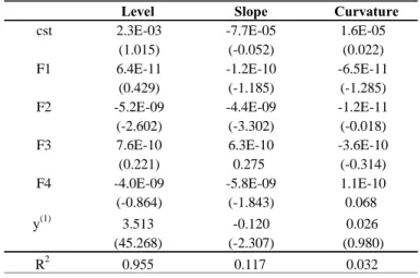
As of the latent yield curve assessment, the term structure is derived in three components (level, slope and curvature), which explains the biggest part of the variation of the yields. Table 8 relates the factors extracted from the dataset with the latent factors of the traditional models. Firstly, the level, slope and curvature are estimated using Diebold-Li model. Then, we regress these latent
factors onto the FAVAR’s factors . These regressions are displayed in the table below. It is interesting to note that the FAVAR’s factors explain 95.5% of the level component variation, but only 11.7% and 3.2% of the slope and curvature variation respectively, what can suggest that slope and curvature could be least related to the economic environment variations.
Table 9 - Regression of latent yield factors on the model factors
Level Slope Curvature
cst 2.3E-03 -7.7E-05 1.6E-05
(1.015) (-0.052) (0.022)
F1 6.4E-11 -1.2E-10 -6.5E-11
(0.429) (-1.185) (-1.285)
F2 -5.2E-09 -4.4E-09 -1.2E-11
(-2.602) (-3.302) (-0.018)
F3 7.6E-10 6.3E-10 -3.6E-10
(0.221) 0.275 (-0.314)
F4 -4.0E-09 -5.8E-09 1.1E-10
(-0.864) (-1.843) 0.068
y(1) 3.513 -0.120 0.026
(45.268) (-2.307) (0.980)
R2 0.955 0.117 0.032
5. Out-of-sample forecasts for the Brazilian Yield Curve
One of the premises for the application of the FAVAR approach developed by Bernanke et al. (2005) is that the local central bank analyses a vast dataset of information to establish the short-term interest rate on its economy. In part 4 of this dissertation, it was shown that the NA-FAVAR model is an interesting model to fit the yield curve in-sample, and, doing so, it is also a good tool to investigate relationships between the yield curve and the macroeconomic environment. The current part studies the application of the model to forecast the yield curve one month, six months and twelve months ahead and was carried out in the period of January 2003 to May 2016.
The forecast process of the no-arbitrage factor-augmented VAR is described as follows. The yields are estimated as of:
𝑦̂𝑡+ℎ|𝑡(𝑛) = 𝑎̂𝑛+ 𝑏̂𝑛´𝑍̂𝑡+ℎ|𝑡 (10)
where Z is a vector with lagged and contemporaneous principal components and also the one-month interest rate, estimated until period t. The parameters 𝑎̂𝑛 and 𝑏̂𝑛´ were estimated by applying a VAR on the states, and minimising the fitting errors, exactly as shown in part 4.
The parameters 𝑍̂𝑡+ℎ|𝑡 of the states are calculated by iterating forward equation (2), i.e.:
𝑍̂𝑡+ℎ|𝑡 = 𝚽̂ℎ𝑍𝑡+ ∑ℎ−1𝑖=0 𝚽̂ 𝝁𝑖 (11)
Hannan-Quinn criterion is used to estimate the number of lags for the FAVAR equation, with a maximum of 12 month lags.
Figure 3 - Forecast results – NA-FAVAR – one month ahead
Table 10 provides the root mean squared errors (RMSE) from both models, showing that Diebold-Li models deliver a better out-of-sample forecast performance for one month ahead for all maturities, which was expected due to the lower volatility of the interest rates in small periods of time.
Table 10 - RMSE out-of-sample results – one month ahead Maturity 1 2 3 4 5 6 7 8 Diebold Li 0.0182 0.0189 0.0192 0.0194 0.0195 0.0197 0.0198 0.0199 NA-FAVAR 0.0082 0.0080 0.0084 0.0091 0.0098 0.0106 0.0113 0.0119 Maturity 9 10 11 12 24 36 60 Diebold Li 0.0202 0.0204 0.0206 0.0208 0.0226 0.0246 0.0269 NA-FAVAR 0.0124 0.0129 0.0134 0.0138 0.0145 0.0137 0.0147
Figure 5 displays the yield curve prediction delivered by both models for six month ahead forecast. Surprisingly, the NAFAVAR model delivers a lower RMSE (Table 10) than Diebold-Li’s for all maturities, what gives support for the development of factor models based on large macroeconomic datasets in order to predict interest rates in a data-rich environment as suggested by Bernanke (2005).
Figure 4 - Forecast results – NA-FAVAR – six months ahead
Table 11 - RMSE out-of-sample results – six months ahead
Maturity 1 2 3 4 5 6 7 8 Diebold Li 0.0237 0.0245 0.0248 0.0249 0.0251 0.0252 0.0253 0.0252 NA-FAVAR 0.0238 0.0222 0.0213 0.0206 0.0203 0.0202 0.0202 0.0203 Maturity 9 10 11 12 24 36 60 Diebold Li 0.0255 0.0256 0.0257 0.0257 0.0265 0.0279 0.0296 NA-FAVAR 0.0202 0.0201 0.0200 0.0198 0.0163 0.0151 0.0153
Figure 5 provides the forecast of the yield curve twelve months ahead for both models. In this case, NAFAVAR results outperformed the competitor model only for the case of higher maturities. It is also interesting to notice that the NAFAVAR model seems to be well adapted to a high volatile
environment.
Figure 5 - Forecast results – NA-FAVAR – twelve months ahead
Table 12 - RMSE out-of-sample results – twelve months ahead
Maturity 1 2 3 4 5 6 7 8 Diebold Li 0.0276 0.0284 0.0287 0.0288 0.0290 0.0291 0.0292 0.0292 NA-FAVAR 0.0325 0.0288 0.0266 0.0250 0.0241 0.0236 0.0231 0.0227 Maturity 9 10 11 12 24 36 60 Diebold Li 0.0294 0.0294 0.0295 0.0295 0.0295 0.0300 0.0309 NA-FAVAR 0.0220 0.0214 0.0208 0.0201 0.0159 0.0153 0.0152
6. Conclusion
This dissertation made an effort to adapt the no-arbitrage factor-augmented vector autoregression model suggested by Moench et al. (2008) to the Brazilian term structure in a data rich environment. The model used the FAVAR approach to model the yield curve in the short-term (Bernanke et al. 2006), and the no-arbitrage concept to estimate the long-term yield curve, as suggested by Ang et al. (2006), summarised by Moench (2008). The model, applied to the Brazilian economy, seems to explain the yield curve rather accurately and the out-of-sample results for some maturities show lower RMSE than the competitor model, Diebold-Li’s model, capturing part of the variation of the interest rates. It is also interesting to analyse that the NAFAVAR model seems to be useful in a high volatile environment such as the Brazilian interest rate market, which was predicted by Moench (2008).
References
Ang, Andrew, Piazzesi, Monika, 2003. A no-arbitrage vector autoregression of term structure dynamics with macroeconomic and latent variables. Journal of Monetary Economics. 50 (4), 745-787.
Ang, Andrew, Piazzesi, Monika, Wei, Min, 2006. What does the yield curve tell us about GDP growth? Journal of Monetary Economics. 127 (1-2), 359-403.
Bernanke, Ben S., Boivin, Jean, Eliasz, Piotr S., 2005. Measuring the effects of monetary policy: A factor-augmented vector autoregressive (FAVAR) approach. The Quarterly Journal of Economics. 120 (1), 387-422.
Bernanke, Ben S., Boivin, Jean, 2003. Monetary policy in a data-rich environment. Journal of Monetary Economics. 50 (3), 525-546.
Bernanke, Ben S., Reinhart, Vincent R., Sack, Brian P., 2004.Monetary policy alternatives at the zero bound: An empirical assessment. Brookings Paper on Economic Activity 2, 1-78.
Bliss, Robert R. 1997. Testing term structure estimation methods. Advances in Futures and Options Research 9, 197-231
Davidson, Russell, MacKinnon, James G., 1993. Estimation and inference in Econometrics. Oxford University Press, New York.
Dewachter, Hans, Lyrio, Marco, 2006. Macro factors and the term structure of interest rates. Journal of Money, Credit, and Banking 38 (1), 119-140.
Diebold, Francis X., Li, Canlin, 2006. Forecasting the term structure of government bond yields. Journal of Econometrics 127 (1-2), 337-364
Diebold, Francis X., Rudebusch, Glenn D., Aruoba, Boragan S., 2006. The macroeconomy and the yield curve: A dynamic latent factor approach. Journal of Econometrics 127 (1-2), 309-338 Duffee, Gregory R., 2002. Term premia and interest rate forecasts in affine models. Journal of Finance 57 (1), 405-443.
Fonseca, Marcelo, Pereira, Pedro, 2015. Credit shocks and monetary policy in Brazil: A structural FAVAR approach.
Giannone, Domenico, Reichlin, Lucrezia, Sala, Luca, 2004. Monetary policy in real time. NBER. Macroeconomics Annual 161-225
Moench, Emanuel, Uhlig, Harald, 2005. Towards a monthly business cycle chronology for the euro area. Journal of Business Cycle measurement and Analysis. 2 (1), 43-69.
factor-augmented VAR approach. Journal of Econometrics 146 (2008) 26 - 43
Nelson, Charles R., Siegel, Andrew F., 1987. Parsimonious modelling of yield curves. Journal of Business 60 (4), 473-489.
Stock, James H., Watson, Mark W., 2002a. Forecasting using principal components from a large number of predictors. Journal of the American Statistical Association 97, 1167-1179.
Stock, James H., Watson, Mark W., 2002b. Macroeconomic forecasting using diffusion indexes. Journal of Business & Economic Statistics 20 (2), 147-162.
Vasicek, Oldrich, 1977. An equilibrium characterization of the term structure. Journal of Financial Economics 5 (1977) 177-188.