DOI: 10.7127/rbai.v8n200247
Protocolo 247/14 – 06/10/2013 Aprovado em 30/03/2014
SPATIAL AND TEMPORAL DISTRIBUTION OF THE WATER CONTENT OF A RED-YELLOW ARGISSOL CULTIVATED WITH BEANS (PHASEOLUS
VULGARIS L.) IRRIGATED BY CENTER PIVOT
Elder Sânzio Aguiar Cerqueira1, Daniel Marçal de Queiroz2, Nerilson Terra
Santos3, Nilce Mazarello Mendes Cerqueira4, Raimundo Rodrigues Gomes Filho5, Ely das
Virgens Santos6
ABSTRACT
This study aimed to identify and assess the spatial and temporal distribution of the water content in a red-yellow argissol cultived with bean, irrigated by central pivot. The samplings were made at a depth of 30 cm, in systematic grid of 10.0 by 10.0 m with 108 and 54 sampling points in conventional tillage (CT) and no tillage (NT), respectively, sampled at four stages of crop development: V3 (1st trifoliated leaf), R6 (flowering), R8 (filling of string beans) and R9 (physiological maturity). The water content of the soil was determined by the greenhouse standard method and the analysis of spatial dependence was obtained with the GS+ Program. The semivariograms presented dependence spatial in conventional tillage, adjusting to the spherical model with ranges of 68.5, 78.3, 73.3 and 75.4 m, and in no-tillage system with ranges of 172.3, 210.9, 193.7 and 100.0 m for the steps V3, R6, R8 and R9, respectively. The relationship between the nugget effect and sill indicated that the spatial dependence was strong, lower than 25%. Using the graphical representation of the surface, the area studied presented higher water content at the low elevation and lower water content at the part of high elevation. Overall, the soil water content in CT showed a narrower range of spatial dependence on the scale, compared to soil water content in NT. The spatial distribution mapping of water content in the soil showed that there is a stability of the time variability for water content in the two cultivating systems.
Keywords: agriculture of precision, geoestatistical, irrigation.
1 Prof. Doutor, Deptº de Engenharia Agrícola, UFS, CEP 49100-000, São Cristóvão, SE, Fone (79)21056999, e-mail: eldersanzio@gmail.com
2 Prof. Doutor, Deptº de Engenharia Agrícola, UFV, Viçosa, MG. 3 Prof. Doutor, Deptº de Informática, UFV, Viçosa, MG.
4 Profª. Mestre, Deptº de Direito, Faculdade Pio Décimo, Aracaju, SE. 5 Prof. Doutor, Deptº de Engenharia Agrícola, UFS, São Cristóvão, SE.
DISTRIBUIÇÃO ESPACIAL E TEMPORAL DO TEOR DE ÁGUA DE UM ARGISSOLO VERMELHO-AMARELO CULTIVADO COM FEIJÃO
(PHASEOLUS VULGARIS L.) IRRIGADO POR PIVÔ CENTRAL RESUMO
Este trabalho objetivou identificar e avaliar a distribuição espacial e temporal dos teores de água de um Argissolo Vermelho-Amarelo, cultivado com feijão, irrigado por pivô central. Foram feitas amostragens compostas na profundidade de 30 cm, em grade sistemática de 10,0 por 10,0 m com 108 e 54 pontos amostrais nos plantios convencional (PC) e direto (PD), respectivamente, amostrados nas quatro etapas de desenvolvimento da cultura: V3 (1ª folha trifoliolada), R6 (floração), R8 (enchimento das vargens) e R9 (maturação fisiológica). O teor de água do solo foi determinado pelo método padrão da estufa, e a análise da dependência espacial foi obtida com o Programa GS+. Os semivariogramas, no PC, apresentaram dependência espacial, ajustando-se o modelo esférico com alcances de 68,5, 78,3, 73,3 e 75,4 m, e no PD com alcances de 172,3, 210,9, 193,7 e 100,0 m, para as etapas V3, R6, R8 e R9, respectivamente. A relação entre o efeito pepita e o patamar indicou que a dependência espacial era forte, menor que 25%. Utilizando a representação gráfica da superfície, a área estudada apresentou um maior teor de água na parte de baixa elevação e menor na parte de alta elevação. O teor de água do solo no PC, em geral, apresentou magnitude de dependência espacial à escala menor quando comparada com o teor de água do solo no PD. Os mapeamentos da distribuição espacial do teor de água no solo demonstraram que existe uma estabilidade temporal da umidade nos dois sistemas de plantio.
Palavras-chave: agricultura de precisão, geoestatística, irrigação.
INTRODUTION
The soil, for more uniform in their appearance, it may vary significantly in their physicochemical properties, and one should adopt a methodology for data collection that allow qualify you over the area of interest (PORTUGAL, et al., 2010).
The water, as needed in all physiological and biochemical processes of crop, is one of the
most important process in agricultural production. To meet the needs of the crop, if the water be applied insufficient quantity it results in hidric stress, if applied in large quantities can cause losses by runoff and percolation, with consequences on the quality and crop productivity. A major water application systems is irrigation, it has reduced the frustration risks of crop and it has prompted the producers to invest increasingly in irrigated agriculture. The
application of water in crop according to the need of each installment, due to the variability of soil water content, can promote the achievement of higher yields, water use efficiency and economic return, but most managements systems irrigation do not take into account this variability, generally applying the same irrigation depth in all area to be irrigated. The spatial variability of soil water could allow a more adequate irrigation management, and maintenance of water content always an interval where there was no excess or energy expenditure on the part of the crop to extract the water from the soil.
For the study of spatial distribution, classical statistics is not appropriate, considering that all observations are independent. In this case, the use of geostatistics has been instrumental, since it takes into account the geographical location and spatial dependence between observations. According to Ortiz (2002), studies using geostatistics to characterize the variability of soils have become increasingly frequent. Besides characterizing a region, knowledge of the variability of soil may indicate the amount and distribution of samples to be removal, allowing better detail of the area and results. Gajem et al. (1981), using sample spacing of 2 m, they identified models for semivariograms of soil moisture, with a range of about 30 m and found significant variability in
the data. Chen et al. (1995) concluded that one must consider the spatial variability in the experimental design for estimating the number of samples of soil moisture. Libardi et al. (1986) worked with samples taken every 0.5 m along a transection of 150 m, seeking to assess the spatial variation of moisture and concluded that the range values were 16 m for moisture. Vauclin et al. (1983) studied the spatial variation of the content water and stored and verified that all properties presented a spatial dependent, reaching between 25 and 50 m. Ferraz et al. (2012) and Silva et al. (2010) evaluated the spatial variability of yield of the coffee crop, found different values of nugget effect and range.
The spatial variability of water content in the soil, using geostatistical methods (CARVALHO et al., 2013), can be an important tool to predict the locations that require monitoring of soil moisture to promote better management of the irrigation system, which would prevent water waste, reduce energy consumption and to obtain better crop production on site.
Therefore, the aim of this study was to identify and analyze the spatial and temporal distribution of the water content of a Red-Yellow Argissol cultivated with beans (Phaseolus vulgaris L.) irrigated by center pivot.
MATERIALS AND METHODS
This work was conducted in the experimental field of the Plant Science Department, Federal University of Viçosa, municipality of Coimbra, MG, in the period from July to November of 2003, comprising the geographical coordinates of WGS 84 datum: 20° 49'51 "to South latitude, 42° 45'57 "west longitude from Greenwich and altitude of 721 m above mean sea level. The experiment used 75% of an area of 2.72 ha irrigated by center pivot being 1.36 ha cultivated with conventional tillage (PC) and 0.68 ha cultivated with no tillage (NT). The soil was characterized as Red-Yellow Argisol, terrace phase. The relief in the experimental area is flat, and its largest slope does not exceed 0.02 m m-1, located in conventional tillage in the east-west direction. We used the bean cultivar Carioca commercial group of type BRSMG Talisman.
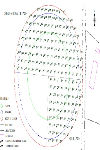
Sampling was carried out according to a grid of 10.00 per 10.00 m (Figure 1), totaling 108 sampling points for CT and 54 sampling points for NT. 688 soil samples were collected during the five stages of crop development. All georeferenced points were located with Total Station and the soils collects were made with two soil samples at each site at a depth of 0-15 cm and 15-30 cm, which were homogenized. The samples were used to determine the water
content of the soil by greenhouse standard method. (EMBRAPA, 1997).
Figure 1 – Scheme of the mesh used in soil sampling to determine the water content in conventional tillage (CT) and no tillage (NT).
The geostatistical study used for the values of soil water content, supplied the following stages of development of the bean: V3 (first trifoliate leaf), R6 (flowering), R8 (filling of string beans) and R9 (physiological maturity). (SCHOONHOVEN e PASTOR-CORRALES, 1987).
RESULTS AND DISCUSSION
The descriptive statistic for values of water content, based on dry weight, in the five stages of crop development is shown in Table 1. The smallest coefficient of variation was found in V3 (CV = 15.49%) and V3 (CV = 8.91%) CT and NT, respectively. The R6, R8 and R9 steps presented on CT the coefficient of variation with 17.15, 15.74 and 20.62%, and on NT 9.28, 10.82 and 12.63%, respectively. There is a greater dispersion of the observed values around the arithmetic mean for the CT in relation to NT. This average dispersion can also be verified by the minimum and maximum values of each stage.
Table 1 – Statistics of water content in the soil
(g/100g) in tillage conventional and no tillage in their respective stages
Tillage Convencional No Tillage
V3 R6 R8 R9 V3 R6 R8 R9 X 27.70 27.17 29.61 24.97 34.81 34.26 36.50 29.92 σ 2 18.44 21.70 21.72 26.52 9.61 10.13 15.57 14.33 σ 4.29 4.66 4.66 5.15 3.10 3.18 3.95 3.78 CV 15.49 17.15 15.74 20.62 8.91 9.28 10.82 12.63 Mnimum Value 18.61 19.43 21.89 17.25 25.51 24.62 28.89 20.21 Maximum Value 37.38 37.23 41.90 41.31 41.27 41.11 45.73 38.78 n 108 108 108 108 53 54 54 54 Cs (error) (0.23) 0.20 (0.23) 0.62 (0.23) 0.71 (0.23) 1.04 (0.33) -0.45 (0.32) -0.40 (0.32) 0.23 (0.32) 0.10 Cc (error) (0.46) -0.70 (0.46) -0.45 (0.46) -0.30 (0.46) 0.33 (0.64) 0.45 (0.64) 0.32 (0.64) -0.71 (0.64) -0.38
where, V3, R6, R8 and R9 – stages of crop development; X - average; σ2 – variance; σ – standard deviation; CV –
coefficient of variation; n - number of samples; Cs - asymmetry coefficient; and Cc - kurtosis coefficient.
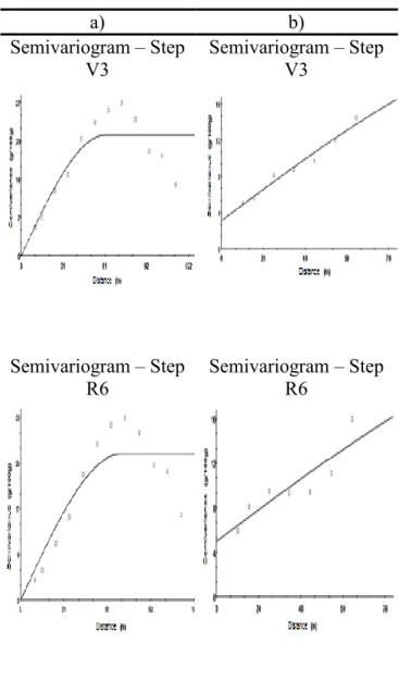
The parameters and adjusted models and selected of the semivariograms of soil water contents obtained experimentally in four stages of crop development for the CT and NT are shown in Table 2 and Figure 2.
It is observed in Table 2 and also in Figure 2, that the nugget effect (C0) on the CT is smaller, relative to NT. It may be due to small structures of straw on the coverage of the NT, they are not captured by the scale of adopted sampling.
The semivariogram on CT presented spatial dependence, adjusting the spherical model with ranges of 68.5, 78.3, 73.3 and 75.4 m, and on NT with ranges of 172.3, 210.9, 193.7 and 100.0 m for steps V3, R6, R8 and R9, respectively. This difference between the two tillage systems is probably due to the greater capacity of water retention in the soil in NT, in function on the straw layer, resulting in higher amplitude spatial dependence, ie, even with a larger grid still detects the spatial variability of the water content of the soil.
Table 2 – Model and parameters of
semivariograms of the experimental data of particle size, on the system conventional tillage (CT) and no tillage (NT)
Steps Models Nugget Effect (Co)
Landing
(Co+C) Range (Ao) *r
2 (%) *RSS IDE(%) V3 (CT) Spherical 0.01 22.93 68.50 87.3 57.9 0.04 R6 (CT) Spherical 0.01 28.98 78.30 91.9 87.5 0.03 R8 (CT) Spherical 0.01 28.02 73.30 85.3 139.0 0.04 R9 (CT) Spherical 0.10 34.78 75.40 87.7 185.0 0.29 V3 (NT) Spherical 3.13 23.24 172.30 96.8 2.19 13.47 R6 (NT) Spherical 4.91 24.51 210.90 78.8 11.80 20.03 R8 (NT) Spherical 7.06 36.11 193.70 94.2 6.48 19.55 R9 (NT) Spherical 2.60 25.19 100.00 99.8 0.507 10.32
*r2 is the coefficient of determination, and RSS is the sum
of squares of waste.
By analyzing the scope range of the four stages of crop development to the soil water content, on the CT, it was noticed that the scope varied from 68.5 to 78.3 m. Therefore, study of soil water content should not be done with grid greater than 68.5 m, as there is a risk of losing information about the spatial dependence. In the NT system, it was realized that the scope ranged from 100.0 to 210.9 m and it should not do the study of soil water content with grid greater than 100.0 m, thus also runs the risk of losing information about the spatial dependence.
a) b) Semivariogram – Step V3 Semivariogram – Step V3 Semivariogram – Step R6 Semivariogram – Step R6 Semivariogram – Step R8 Semivariogram – Step R8
Semivariogram – Step
R9 Semivariogram – Step R9
Figure 2 – Semivariogram of the experimental data of soil water content, in the systems: a) conventional tillage (CT) and b) no tillage (NT)
The index of spatial dependence (ISE) defined by Cambardella et al. (1994), allowed us to classify the spatial dependence of soil water content as strong spatial dependence, ie, the nugget effect was less than 25% of the landing for the CT and NT in four stages of crop development. Although the ISE of NT is in the range of strong spatial dependence, according to the classification used, its average value is about 186 times the value of the CT of ISE, showing that in areas of NT, the control of the soil water content can have grid larger, reducing the cost of controlling of this variable.
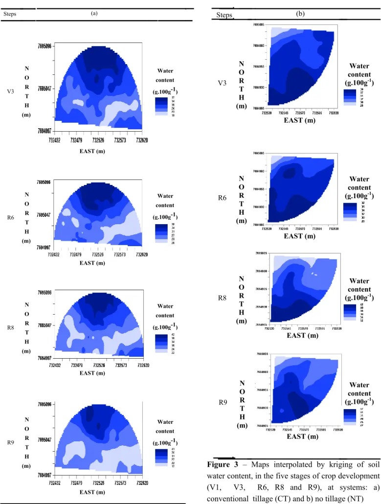
The maps of soil water content in the four stages of crop development, CT and NT (Figure 3) show a big difference in this variable between the two systems. It is noted that on PC, the soil water content has a variation between 17 and 42 g (100 g)-1 and the NT between 22 and 42 g (100
g)-1. This fact corresponds to a soil water content
lower 22.7% on CT in relation to the NT,
because the coverage with straw layer results in a slower evaporation of water in the NT.
The values of soil water content of CT (Figure 3a) indicate that the highest values tend to concentrate in the top half of the map corresponding to the north face of the area. While the positions occupied by the values of soil water content for NT (Figure 3b) show higher values of water content in the lower half of the map corresponding to the south face of area.
In general, it is observed that on the maps of soil water content on the CT and NT, there are small differences between the stages of crop development. There is greater variation of soil water content on CT in relation to NT.
The knowledge of the existence of spatial variability can be applied in precision agriculture, for example, from the use of maps of soil water content. The correct interpretation of such maps, can lead to more efficient use of existing natural resources, thus providing lower cost of production, while preserving the environment.
The spatial dependence detected on the map of soil water content is a clear indication that the farmer will have to conduct a management water use in a different way compared to their all area. This result has found a similarity between the maps in the four stages of crop development in relation to the concentration trend of higher values of water content.
V3 N O R T H (m) EAST (m) Water content (g.100g-1) N O R T H (m) EAST (m) Water content (g.100g-1) R6 N O R T H (m) EAST (m) Water content (g.100g-1) N O R T H (m) EAST (m) Water content (g.100g-1) R8 N O R T H (m) EAST (m) Water content (g.100g-1) N O R T H (m) EAST (m) Water content (g.100g-1) R9 N O R T H (m) EAST (m) Water content (g.100g-1) N O R T H (m) EAST (m) Water content (g.100g-1)
Figure 3 – Maps interpolated by kriging of soil water content, in the five stages of crop development (V1, V3, R6, R8 and R9), at systems: a) conventional tillage (CT) and b) no tillage (NT)
V3
R6
R8
The maps generated for the water content may indicate to the farmer how much water it should be applied in each region of the map. Furthermore, the results indicate that the amount to be applied in each region of the map tend to be the same along the crop development.
CONCLUSIONS
The mapping of the spatial distribution of soil water content showed that there is stability in the temporal variability of soil moisture in both tillage systems, allowing to predict where to install sensors for the determination of soil water content for irrigation monitoring in real time and may be used to define a irrigation management differentiated in the area.
The soil water content variable in conventional tillage, in general, presents magnitude of spatial dependence to a lesser extent compared with the soil water content variable in no tillage.
The model of spatial variability can be applied in precision agriculture using cross of informations as maps of water content in the soil, expecting that the spatial variability contributes with agricultural decisions and with better use of
soil and water resources.
Amplitude variations of the spatial dependence between the four stages of crop development, indicate that inferences about the soil water content variable should consider the applied management system, the spatial variation of this attribute and the steps of the development at the crop cycle.
REFERENCES
ALVAREZ, V. H. e CARRARO, I. M. Variabilidade do solo numa unidade de amostragem em solos de Cascavel e de Ponta Grossa – Paraná. Revista Ceres, Viçosa, MG, v. 23, 1976.
CAMBARDELLA, C. A.; MOORMAN, T. B.; NOVAK, J. M.; PARKIN, T. B.; KARLEM, D. L.; TURCO, R. F.; KONOPA, A. E. Field-scale variability of soil properties in central Iowa soil.
Soil Science Society of American Journal,
Madison, v. 58, p. 1501-1511, 1994.
CARVALHO, L. C. C.; SILVA, F. M.; FERRAZ, G. A. S.; SILVA, F. C.; STRACIERI, J. Variabilidade espacial de atributos físicos do solo e características agronômicas da cultura do café. Coffee Science, Lavras, v. 8, n. 3, p. 265-275, jul./set. 2013.
CHEN, J.; HOPMANS, J. W.; FOGG, G. E. Sampling design for soil moisture measurements in large field trials. Soil Science, v. 159, n. 3, p. 155-161, 1995.
SCHOONHOVEN, V. A. e PASTOR-CORRALES, M. A. Sistema estándar para la evaluación de germoplasma de fríjol. Cali: Centro Internacional de Agricultura Tropical, 1987. 56p.
EMBRAPA – EMPRESA BRASILEIRA DE PESQUISA AGROPECUÁRIA. Manual de métodos de análise de solo. 2. ed. Rio de Janeiro: Centro Nacional de Pesquisa de Solos, 1997. 212 p.
FERRAZ, G. A. S.; SILVA, F. M.; CARVALHO, L. C. C.; ALVES, M. C.; FRANCO, B. C. Variabilidade espacial e temporal do fósforo, potássio e da produtividade de uma lavoura cafeeira.
Engenharia Agrícola, Jaboticabal, v. 32, n. 1, p.
140-150, jan./fev. 2012.
GAJEM, Y. M.; WARRICK, A. W.; MYERS, D. E. Spatial dependence of physical properties of a typic torrifluvent soil. Soil Science Society
of American Journal, v. 45, n. 4, p. 709-715,
1981.
GS+. GS+ Geostatistics for the Environmental Sciences. Version 5.3.1. Gamma Design Software, Michigan, 2000.
GUIMARÃES, E. C. Variabilidade espacial de atributos de um latossolo vermelho escuro textura argilosa da região do cerrado, submetido ao plantio direto e ao plantio convencional. Campinas, SP: FEAGRI/UNICAMP, 2000. Tese (Doutorado).
LIBARDI, P. L.; PREVEDELLO, C. L.; PAULETTO, E. A.; MORAES, S. O. Variabilidade espacial da umidade, textura e massa específica de partículas ao longo de uma transeção. Revista Brasileira de Ciência
do Solo. Campinas, SP, v. 10, n. 2, p. 85-90,
1986.
ORTIZ, G. C. Aplicação de métodos geoestatístico para identificar a magnitude e a estrutura da variabilidade espacial de variáveis físicas do solo. Piracicaba, SP: Escola Superior de Agricultura “Luiz de Queiroz”, 2002. Dissertação (Mestrado).
PORTUGAL, A. F.; COSTA, O. D. V.; COSTA, L. M. Propriedades físicas e químicas do solo em áreas com sistemas produtivos e mata na região da zona da mata mineira. Revista Brasileira de
Ciências do Solo, 34:575-585, 2010.
SILVA, F. M.; ALVES, M. C.; SOUZA, J. C. S.; OLIVEIRA, M. S. Efeitos da colheita manual na bienalidade do cafeeiro em Ijaci, Minas Gerais. Ciência e
Agrotecnologia, Lavras, v. 34, n. 3, p.
625-32, maio/jun. 2010.
VAUCLIN, M.; VIEIRA, S. R.; VAUCHAUD, G.; NIELSEN, D. R. The use of cokriging with limited field observation. Soil Science Society of
America Journal, Madison, v. 47, p. 175-184,