Juliana Pinheiro Pires Supervisors:

(1)

UNIVERSITY

OF

BRASILIA

POST

GRADUATION

PROGRAM

IN

CHEMISTRY

RECONSTRUCTION

OF

NEOGENE

SEA

SURFACE

TEMPERATURES

IN

CEARA

RISE

(SOUTH

ATLANTIC)

BASED

ON

ALKENONES

Juliana

Pinheiro

Pires

Supervisors:

Prof.

Dr.

Fernanda Vasconcelos de Almeida

Dr. Jung-Hyun Kim

Brasilia

–

DF

(2)

JULIANAPINHEIROPIRES

RECONSTRUCTIONOFNEOGENESEASURFACETEMPERATURESIN CEARARISE(SOUTHATLANTIC)BASEDONALKENONES

Dissertationsubmittedto theInstitute

of Chemistry, University of Brasilia,

asa partial requirement for obtaining

titleofMasterinChemistry.

Area of concentration: Analytical

Chemistry.

Supervisors: Prof. Dr. Fernanda

Vasconcelos de Almeida and Dr.

Jung-HyunKim.

Brasilia -DF

(3)

APPROVAL

SHEETF

Communicate the approval of the Dissertation Defesnse of Master

of the student Juliana Pinheiro Pires, registration nº. 13/0086053, entitled

"Reconstruction of Sea Surface Temperatures Neogene In Ceara Rise

(South Atlantic ) Based On Alkenones " presented at PADCT room of the

Institute of Chemistry ( IQ ) of the University of Brasilia ( UnB ) on March 5,

2015 .

Prof. Dr. Fernanda Vasconcelos de Almeida

President of the sink (IQ/UnB)

Prof. Dr. Valéria Regina Bellotto

Titular Member (IQ/UnB)

Prof. Dr. Poliana Dutra Maia

Titular Member (FUP/UnB)

Prof. Dr. Marly Eiko Osugi

Substitute Member (IQ/UnB).

(4)

I dedicatethisthesistomyparentsRobertoandMariaGeralda,

whogavemeunconditionalsupportanddonotmeasureeffortsto

therealizationofmydreams.

DedicoessadissertaçãoaosmeuspaisRobertoeMariaGeralda,

peloapoioincondicionalepornãomediremesforços para

(5)

ACKNOWLEDGMENTS

Thank first to God for giving me strength and wisdom to walk the paths of

graduationandmasterandovercomethedifficulties.

To my parents, who were with me in the moments that I most needed and

advised me in the most difficult moments. You are responsible for the person I

havebecome.Iloveyou.

To my sister Luciana and my boyfriend Jonatan, who endured my moments of

anxietyandstress.Withoutthelove,friendship andfellowship ofyou,Icouldnot

concludethisimportantstageofmylife.

To the teacher Dr. Fernanda, who welcomed me in the laboratory and was

always willing to listen and help me. Thank you for being my supervisor and

givingmeallthesupportnecessaryfortheconclusionofthismaster.

Tomysupervisor Dr.Jung-HungKim,forsharingherexperienceandwisdom.

To Elsbeth Van Soelen, for all patience, attention and dedication and for being

mypartner inallstagesofthismaster.Thankyou.

To theAQQUA teachers, Valéria, Jez, Fernando, Ana Cristiand Alexandre, for

beingalwaysavailabletohelpandanswerquestions.

To my colleagues in AQQUA Group, especially Angela, Gabriel, Tati, Rosy,

Carla,Victor, Milena andDaniel, forsharing greatmomentsof relaxation, laugh

andforbealwayswillingtohelpme.

ToCNPq,forfinancialsupport.

TotheClimAmazon Projectforfinancialsupport.

ToUNBandtheInstituteofChemistry.

Andtoallwhowerepartofthishistory.

(6)

AGRADECIMENTOS

Agradeço primeiramente a Deus, por ter me concedido força e sabedoria para

trilharoscaminhos dagraduaçãoedomestradoevencerasdificuldades.

Aosmeus pais, queestiveram aomeu ladonos momentos quemaisprecisei e

meaconselharamnosmomentosmaisdificeis. Vocêssãoosresponsáveispela

pessoaquemetorneiedevoaosdoistudoquejáconsegui.Amovocês.

À minha irmã Luciana e ao meu namorado Jonatan, que aguentaram meus

momentos de ansiedade e de estresse. Sem o carinho, a amizade e o

companheirismodevocês,eunãoconseguiriaconcluirestaetapatãoimportante

deminha vida.

À professora Dra. Fernanda, que me acolheu no laboratório e sempre esteve

dispostaameouvireajudar.Obrigadaporserminhaorientadoraemedartodoo

suporteparaqueessemestradoserealizasse.

ÀminhacoorientadoraDra.Jung-HungKim,pelaexperiência esabedoria.

ÀElsbethVanSoelen,portodapaciência,atenção ededicação eporserminha

companheiraemtodasasetapasdessadissertação.Muitoobrigada.

AosprofessoresdoAQQUA,Valéria,Jez,Fernando,AnaCristieAlexandre,por

estaremsempredispostosaajudaretirardúvidas.

Aos colegas do Grupo AQQUA, especialmente Angela, Gabriel, Tati, Rosy,

Carla, Victor, Milena e Daniel, por proporcionarem ótimos momentos de

descontração,boasrisadaseestaremsempre dispostosameajudar.

AoCNPqeaoProjetoClimAmazon,peloauxíliofinanceiro.

ÀUnBeaoInstitutodeQuímica.

Eatodosquefizerampartedessahistória.

(7)

“Therealvoyage ofdiscoveryconsistsnotinseekingnewlandscapes,butin

havingneweyes.”

MarcelProust

“Averdadeira viagemdedescobrimentonãoconsisteemprocurarnovas

paisagens,masemternovosolhos.”

(8)

ABSTRACT

PIRES, J. P. Reconstruction ofNeogene sea surface temperatures inCeara

Rise (South Atlantic) based on alkenones. 2015. Dissertation (Master in

Chemistry)–UniversityofBrasilia,Brasilia,2015.

The Ceara Rise is a seismic peak located in the Atlantic Ocean and

receives both marine and terrigenous sediments. These sediments are

important for understanding the paleoclimatic and paleo-environmental

conditions in the ocean. With the goal of reconstructing the past sea surface

temperature (SST), the lipid biomarkers n-alkanes and alkenones were

analyzedinsedimentsofCearaRise.Thequantificationofbothbiomarkerswas

performed by Gas Chromatography with Flame Ionization Detector (GC-FID).

For the n-alkanes, analytical curves, which resulted in acceptable figures of

merit by official norms and the National Institute of Metrology, Quality and

Technology(Inmetro) were built. Because there is no alkenone standard

commercially available for the construction of analytical curves for alkenones,

thequantificationwasdonebycomparison oftheareasofanalytestothearea

ofastandard ketonecommerciallyavailable. Thequantification bycomparison

areaswasvalidatedbyT-Test,inwhichthevaluesofconcentrationofn-alkanes

obtained for this quantification method were compared with the calculated

concentrations from analytical curves, which led to satisfactory results. The

n-alkanes were evaluated according to the proxies Carbon Preference Index

(CPI) and Average Carbon Length (ACL). The results suggest that the main

source of organicmatter in the studied sediments originates from terrigenous

material transported by rivers and by wind action. The , proxy that use the

concentration of alkenones to calculate the SST, was used for climatic

reconstructionoftheregion.Theconcentrationrangeofalkenoneswas0.001to

0.516 µg g-1. According to the result of proxy, the estimated lowest

temperature was 22.5 °C, toward the end of Early Miocene, while the highest

temperature,28.5°C,washeldathalftheEarlyOligocene.

(9)

LIST

OF

FIGURES

Figure 1. Structure of methyl (Me) and ethyl (Et) long-chain alkenones. The

position of the double bounds are indicated by red circles. Adapted from

CASTAÑEDAetal.,2008... 20

Figure2.Illustrationofthe SSTproxy.Ontheleft,gaschromatogramofa sample with relatively cooler signal than the chromatogram on the right. Adaptedfrom CASTAÑEDAetal.,2008... 21

Figure3.LocationofCeara RiseintheAtlantic Ocean.AdaptedfromCURRY etal.,1994... 24

Figure4.StructuralmapoftheequatorialAtlanticandoftheboundariesofthe CearaRiseandSierraLeone Rise,fromKUMARetal.,1977... 25

Figure 5. Pesperctive view of Ceara Rise, ODP 154, site 925. Adapted from CURRYetal.,1994... 28

Figure6.ExtractsofsedimentsamplesfromCearaRise... 32

Figure 7. (A) Sodium sulfate column prepared in a Pasteur pipette and (B) systemtotransfertheextracttothevialthroughthecolumn... 33

Figure8.Generalschemeoftheanalytical workflow... 35

Figure9.Gaschromatographywithflameionization detector(GC-FID)Agilent 7650A... 37

Figure10.Recoveryfactors(%)ofrotoevaporationand concentrationstepsof thesolventwithanitrogenflow... 46

Figure 11. Comparing the concentrations obtained for different number of extractionsofalkenones……….…..46

Figure 12. Comparing the concentrations obtained for different number of extractionsofn-alkanes………... ……46

Figure13.Typicalchromatogramobtainedforn-alkanesextracts(sampleCRA 5R4)... 50

Figure14.Analyticalcurve ofC-22... 52

Figure15.Analyticalcurve ofC-23... 52

(10)

Figure17. Analyticalcurve C-25... 52

Figure18.Analyticalcurve ofC-26... 52

Figure 28. Representative chromatogram of sediment sample containing alkenones... 64

Figure 29. Calculated CPI values along the record at sites 925 A and 925 B, situatedatCearaRise... 70

Figure 30. ACL values calculated over the record sites 925 A and 925 B, situatedatCearaRise... 71

(11)

LIST

OF

TABLES

Table 1.Informationaboutthe CoreRecoveryA (CRA):period, age,sample´s

nameanddepth... 29 Table 2.Informationaboutthe CoreRecoveryB (CRB):period, age,sample´s

nameanddepth... 30

Table3.Basicinformationofthestudiedexplorationcore... 31 Table4. Informationaboutthestandardusedtomaketheanalyticalcurve..36 Table5.ChromatographicparametersoftheGC-FIDusedinthedetermination

ofalkenonesandn-alkanes... 38

Table6. Valuesofcorrelationcoefficientsobtainedfromtheanalyticalcurves.42 Table 7 Estimation of SD and CV to the standards of squalene and

nonadecanonethroughtherepeatabilityofareas(inpicoampere(pA))... 43

Table8.ValuesofT-calculatedfortheaveragecomparisontest... 45 Tabela9.LODandLOQobtainedfornonadecanoneandsqualene... 48 Table 10.Retention times (min) of n-alkanes used in the construction of

analyticalcurve………...49

Table 11. Concentrations (µg mL-1) and total areas of the external standard

analyticalcurve ofn-alkanesused………..………….…...50

Table12.Weightandsedimentconcentrations(µgmL-1)of14n-alkanesinthe

sediment samples of the cores CRA and CRB of Ceara Rise obtained by

interpolationintheanalytical curves... 56 Table 13. Concentrations (µg mL-1l) of n-alkanes in 14 samples of sediment

coresCRAandCRBofCearaRiseobtainedbycomparisonwiththeareaofthe

internalstandard... 60

Table 14.Concentrations(µgmL-1)ofalkenonesinsedimentsamplesofcores

CRA and CRB of Ceara Rise obtained by comparison with the area of the

internalstandard... 65

Table15.Concentrations(µgmL-1)ofalkenonesinsedimentsamplesofcores

CRA and CRB of Ceara Rise obtained by comparison with the area of the

(12)

LIST

OF

ABBREVIATIONS

AND

ACRONYMS

ANVISA NationalHealthSurveillanceAgency

ACL AverageChainLength

AQQUA GrupodeAutomação,QuimiometriaeQuímicaAmbiental

Be Berilium

C-22 N-docosane

C-23 N-tricosane

C-24 N-tetracosane

C-25 N-pentacosane

C-26 N-hexacosane

C-27 N-heptactosane

C-28 N-octacosane

C-29 N-nonacosane

C-30 N-triancontane

C-31 N-hentriacontane

C-32 N-dotriacontane

C-33 N-titriacontane

C-34 N-tetratriacontane

C-35 N-pentatriacontane

C37:2 Alkenonewith37carbonsandtwounsaturations

C37:3 Alkenonewith37carbonsandthreeunsaturations

C37:4 Alkenonewith37carbonsandfourunsaturations

C38:2 Alkenonewith38carbonsandtwounsaturations

C38:3 Alkenonewith38carbonsandthreeunsaturations

CRA CoreRecoveryA

CRB CoreRecoveryB

CO2 CarbonDioxide

CV CoefficientofVariation

CPI CarbonIndexPreference

(13)

DSDP DeepSeaDrilling Project

Et Ethyl

FID FlameIonizationDetector

GC GasChromatograph

GDGT GlycerolDiakylGlycerolTetraethers

ICH InternationalConference ofHarmonization

INMETRO InstitutoNacionaldeMetrologia,QualidadeeTecnologia

IS Internal standard

KYR Thousand years

LOD LimitofDetection

LOQ LimitofQuantification

Ma MillionYearsAgo

mbsf Metersbelowseafloor

Me Methyl

MeOH Methanol

Na2SO4 SodiumSulfate

N2 Nitrogengas

NOAA NationalOceanicandAtmosphericAdministration

ODP OceanDrillingProject

OLR OutofLinearRange

pA Picoampere

R Correlation Coefficient

RT RetetionTime

SD StandardofDesviation

SST SeaSurface Temperature

TLE TotalLipidExtract

UCM Unresolved ComplexMixture

UnB Universidade deBrasília

(14)

1. INTRODUCTION...15

2. BIBLIOGRAPHICREVIEW...17

2.1CENOZOICCLIMATE EVOLUTION... 17

2.3. PROXIES CARBON PREFERENCE INDEX AND AVERAGE CHAIN LENGTHANDSOURCEOFN-ALKANES... 22

2.4.STUDYAREA... 24

2.4.1.PREVIOUSWORK... 26

3. MATERIALSANDMETHODS...28

3.1.SAMPLECOLLECTIONANDPREPARATION... 28

3.2.ORGANICGEOCHEMISTRY... 31

3.2.1.CLEANING GLASSWARE... 31

3.2.2.LIPIDEXTRACTIONANDPURIFICATION... 31

3.2.2.1.EXTRACTIONOFALKENONESANDN-ALKANES...32

3.2.2.2.PREPARATIONOFINTERNAL STANDARDS... 33

3.2.2.3.SEPARATIONOFFRACTIONSOFALKENONESANDN-ALKANES33 3.2.3.DETERMINATIONANDQUANTIFICATIONOFALKENONES... 35

3.2.4.DETERMINATIONANDQUANTIFICATIONOFN-ALKANES... 36

3.3.VALIDATION... 38

3.3.1.DETERMINATIONOFOUTLIERSINANALYTICALCURVES... 38

3.3.2.LINEARITY... 39

3.3.3.REPEATABILITYTEST... 39

3.3.4.TTESTFORCOMPARISONOFCONCENTRATIONS... 39

3.3.5.RECOVERYTESTS... 40

3.3.6.LIMITSOFDETECTIONANDQUANTIFICATION... 41

4.RESULTSANDDISCUSSION... 42

4.1.METHODVALIDATION... 42

4.1.1.VERIFICATIONOFOUTLIERS... 42

4.1.2.LINEARITY... 42

(15)

4.1.5.RECOVERYTESTS... 46

4.1.6.LIMITSOFDETECTIONANDQUANTIFICATION... 48

4.2.QUALITATIVEDETERMINATIONOF N-ALKANES... 48

4.3.QUANTITATIVEDETERMINATIONOFN-ALKANES... 51

4.4.QUALITATIVEDETERMINATIONOFALKENONES... 64

4.5.QUANTITATIVEDETERMINATIONOFALKENONES... 65

4.6. PROXIES CARBON PREFERENCE INDEX AND AVERAGE CHAIN LENGTH... 69

4.7.RECONSTRUCTIONOFSST... 71

5.CONCLUSIONS... 75

6.BIBLIOGRAPHICREFERENCE... 77

(16)

1. INTRODUCTION

Studiesbasedonpastclimatechangearefrequentlyusedtounderstand

current climatestrendsand alsomakingforecasts.Themainclimate datareferto

rainfallpatternsandtemperaturevariations(VILLALBAetal.,2009).

Thetoolsproxiesareequationsthatrelateproportionsofmoleculeswith

different environmental conditions. They play an important role in the

reconstruction oftemperature profilesandarewidelyused inpaleoenvironmental

studies asanaturalregisterofenvironmentalchanges(CASTAÑEDAetal.,2008;

MANNetal.,2008).Amongthevariousproxiesappliedtoachievethisgoal,those

using organic molecules considered biomarkers have shown great potential for

application indeterminingthesurfacetemperatureofthesea.

The determination of sea surface temperature (SST) is one of the

fundamentalparameterforthereconstructionofpastclimateconditions,aswellas

for understanding the hydrological cycle and wind systems. (EGLINTON et al.,

2008).

Considering these aspects, the present study aims to evaluate the

temperature changes on sediment core from the Ocean Drilling Program (ODP)

154, site925usinglipidbiomarkers.Site925sedimentsamples wereretrieved in

the Ceara Rise (South Atlantic), located 800 kilometers east of the mouth of

AmazonRiver.Thesedimentscontainorganic matterderivedfrombothterrestrial

and marine sources. Therefore, core site 925 will provide valuable information

whichcanhelptolinkpaleoenvironmentalandpaleoclimaticconditionsonlandto

thoseintheocean.

This study is part of the international project CLIM-AMAZON, the joint

Brazilian-European researchfacility for climate and geodynamic research on the

(17)

i. to set up the analytical structure for the extraction and analysis of

lipid biomarkers in sediment samples in the analytical chemistry

laboratory at the Chemistry Institute in the University of Brasilia

(UnB),AQQUA group;

ii. to analyzen-alkanesandalkenones, twotypesoflipidbiomarkers,

inmarinecoresedimentsofCearaRise(SouthAtlantic)atdifferent

coredepthlevels;

iii. to generate analytical data for reconstruct the past sea surface

(18)

2. BIBLIOGRAPHIC

REVIEW

2.1 CENOZOIC CLIMATE EVOLUTION

The Cenozoic, the most recent era, coversthe period from 65.5 million

yearsago(Ma)topresent(AppendixA).Thiseraisdividedintothreesub-periods:

Paleogene (65.5- 23 Ma),Neogene (23 – 2.5 Ma,the sub-period containing the

Miocene and Pliocene epochs) and Quaternary (2.5 Ma to the present day)

(HELMOND,2010).

TheCenozoicpresentsacomplexclimaticevolutionandthisinformation

isobtained mainlyfromthestudyofdeep-seasedimentcores.In general,climate

changesovertimearedrivenbyshiftinthedistributionofsunlight(LISIECKIetal.,

2007),tectonicprocesses(FEARYetal.,1990)andorbitalcycles(ZACHOSetal.,

2001).

Due to the high temperatures recorded during the early Cenozoic, the

planet was characterized as 'Greenhouse World' (HELMOND, 2010). The

concentrationofgreenhousegases,mostlyfromvolcanicemissions,isamongthe

factsthatledtothishightemperature,becausethepartialpressureofgasessuch

as carbon dioxide (CO2) affects the level of precipitations, the stability of the ice

sheets and atmospheric and oceanic circulation. In a period of less than 10,000

yearsinthetransitionbetweenthePaleoceneandEocene(~55Ma),anincrease

of approximately 5 °C was recorded (ZACHOS et al., 2008).This warming trend

hasspreadfromtheearlyEocene(~50Ma),periodinwhichtherewererecordsof

extremehightemperatures,untiltheOligocene(~33Ma)(PEARSONetal.,2007).

From then, the lowering of the concentration of greenhouse gases has

shownthatclimaticevolution wascharacterizedbyaglobalcoolingtrend,andthis

coincided with the appearance of glaciers inAntarctica (PEARSONet al., 2007).

Thetrendtolowertemperatures, whichpersisteduntilthelateOligocene(FEARY

(19)

concentration of oxygen isotopes (δ18_O), _parameter _used _to _study _changes _in

volume of ice and water temperature (LISIECKI et al., 2007; PEARSON et al.,

2007; ZACHOSet al.,2001;. ZACHOS etal., 2008). Coolinghappenedmilder in

the tropicsbut,atthe poles,ledto adeclineof5-10 °CinSST (PEARSON etal.,

2007).

InthemiddleMiocene (15Ma)andearlyPliocene(6Ma) smallintervals

ofheatwereregistered,resultinginareductioninthevolumeofglaciers.However,

it is observed thatthe general trend in the Cenozoic wasthe globalcooling, due

mainly to the expansion of ocean passages and thermal isolation of Antarctica

(FEARY etal.,1990;ZACHOSetal.,2001;LISIECKIetal.,2007).

The climatic changes that occurred during the Neogene are especially

important because they resulted in significant impacts on the fauna and flora,

givingrisetomodernclimaticregimesandbiomes(PETERetal.,2004).

Itisestimatedthatattheendofthecentury, theconcentrationofCO2in

the atmosphere will be similar to what occurred in the warm period of the early

Pliocene, inwhichtheSST was3 °Cwarmerthan thecurrentlyregistered.Thus,

understanding climate changes that occurred in the Neogene is of fundamental

importancetopredictthefutures climatetrends(HAYWOODetal.,2009).

Theregionalimpactofsuchchanges,forinstanceontheAmazonbasin,

is yet unclear. The marine sediment cores, which contain both terrestrial and

marine organicmatter allow understanding the relationshipbetween the oceanic

and climatic conditions, from the Miocene to the present day. This is possible

through the analysis of organic material recovered outside the Amazon Basin in

Ceara Rise (South Atlantic). Climatic variations in this region may also serve to

understanding climatedynamics that affect variousparts of the globe (BOOT, et

(20)

2.2. LIPID

BIOMARKER

PROXY

FOR

CLIMATE

RECONSTRUCTION

Proxies can relate the variation of temperature with environmental

changes through a calibration, which allows to estimate the climatic conditions

overtheyears(CASTAÑEDAetal.,2008;MANNetal.,2008).

The determination of SST isone of thefundamental parametersfor the

reconstructionofpastconditions,aswellasforunderstandingthehydrologicaland

wind systems(ENGLITON etal.,2008;KIM etal., 2009).SSTalso influencesair

temperature,oncethelandsurfacehasalowerspecificheatthanthewaterbodies

(FRITZSONSetal.,2008).

For the determination of SST, there are temperature proxies that were

developedfromthestudyofgeochemicalproperties, suchastheratioofisotopes

of carbon or oxygen, primary tool for climatic reconstruction of the Cenozoic

(FEARYetal.,1991;ZACHOSetal.,2001).However,proxiesthatuseinformation

at the molecular level are more specific because they do not require many

additionaldatatothedefinitionofprofiles(VILLALBAetal.,2009;CASTAÑEDAet

al., 2008; EGLINTON et al., 2008; EIGENBROD et al., 2010). The biological

markers,knownasbiomarkers,arethemajororganicmoleculesusedforthisform

ofproxy.

Biomarkers are complex organic molecules derived from living

organisms, especially plants and bacteria, which may be deposited with the

sediments and provide environmental information from the time they were

deposited.Theirconcentrationdependsonfactorssuchasoceantemperatureand

lightlevel(CASTAÑEDAetal.,2008;EGLINTONetal.,2008;SMITHetal.,2013;

BLYTH et al., 2008; MEYERS et al.,2003; SACHS et al., 2013; SPERA et al.,

(21)

theypossessahighdegreeofpreservation(CASTAÑEDAetal.,2008;EGLINTON

et al.,2008;BLYTHetal.,2008).

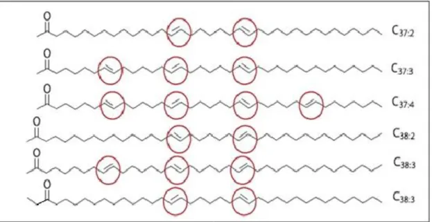
One of the major organic biomarkers for studying paleotemperatures

variationarealkenones,longchainketoneswhichhave37carbonswithtwo,three

orfourunsaturations(C37:2,C37:3andC37:4,respectively)or38carbonswithtwoor

threeunsaturations(C38:2,C38:3,respectively)(Figure1).Theyareproducedmainly

bytwospeciesofunicellular algae:Emilianiahuxluji andGeophyrocpsaoceanica

(CASTAÑEDAetal.,2008;EGLINTONetal.,2008;SACHSetal.,2013;HEBERT

et al., 2003.).These algae reside above the photic zone and require sunlight for

photosynthesis(CASTAÑEDAetal.,2008;EGLINTONetal.,2008;SACHSetal.,

2013).

Figure1.Structureofmethyl(Me)andethyl(Et)long-chainalkenones.Thepositionofthedouble boundsareindicatedbyredcircles.AdaptedfromCASTAÑEDAetal.,2008.

By using the alkenones abundance it is possible to calculate the

unsaturation indexofketones( )(Equation1),aproxydevelopedbyBrasselet

al.in1986andconsideredoneoftheoldestandmostappliedproxiesthatuseratio

of organic compounds (CASTAÑEDA et al., 2008; EGLINTON et al., 2008;

(22)

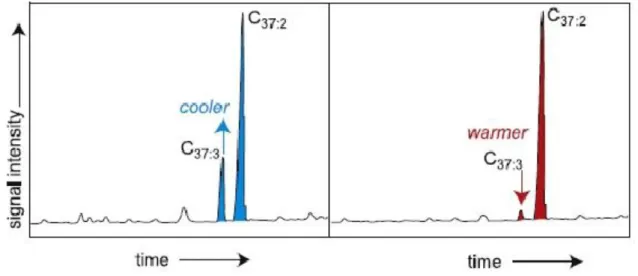
Amarinesediment core studyshowed that the index wassensitive to

paleotemperature fluctuations in the late Pleistocene (BRASSEL et al., 1986),

showingthatwhenthetemperatureoftheseasurfaceincreases,theconcentration

ofC37:3decreasesrelativetotheconcentrationofC37:2(Figure2)(CASTAÑEDAet

al.,2008;EGLINTONetal.,2008).

Figure2.Illustrationofthe SSTproxy.Ontheleft,gaschromatogramofasamplewith relativelycoolersignalthanthechromatogramontheright.AdaptedfromCASTAÑEDAetal.,

2008.

LaterstudiesbyPrahletal.(1987)showed thattheconcentrationof C37:4

in sediments was very low and did not produce significant differences in SST.

Thus, the index developed by Brassel et al. was modified, generating

(Equation2),in which theconcentration ofC37:4isdisregarded (CASTAÑEDA

et al., 2008; SMITH et al., 2013; SACHS et al., 2013). The indexrelates to

(23)

where istheproxythatrelatestheconcentrationofalkenoneswith37carbon

atomsandtwoandthreeunsaturation,[C37:2]and[C37:3]respectively,andSSTis

the sea surfacetemperature (CASTAÑEDAet al.,2008;EGLINTON et al.,2008;

SMITHetal.,2013;PRAHL etal.,2006).

Thisproxypresentsanempiricalrelationshipbetween andSSTandthe

calculated values vary between zero and one. According to the literature, when

assumes avalueequaltooneunit,itfollowsthattheSSTisequivalentto29

°C, with some variations, because the constant calculation can take different

values, which depend on the region where the calibration was performed

(EGLINTONetal.,2008;FRITZSONSetal.,2008;TONEYetal.,2012).

2.3. PROXIES CARBON PREFERENCE INDEX AND AVERAGE

CHAIN LENGTH AND SOURCE OF

N

-ALKANES

The n-alkanes (long-chain hydrocarbons) are biomarkers which provide

important paleoenvironmental informations as well as alkenones. Through

information onthe sizeof thechains ordistribution of thenumberofcarbons it is

possible toidentifywhetherthereisapredominanceofterrigenousmaterialtaken

totheseaorifthesen-alkanesareproducedinwaterbodies(CASTAÑEDAetal.,

(24)

Carbon preferenceindex(CPI) measurestherelativeabundance ofodd over

even carbonchainlengths (CASTAÑEDAetal., 2008;JENG etal., 2006).CPI is

calculatedaccordingtoequation4.

CPI= X (4)

whereC25andC26arerespectivelytheconcentrationofn-alkanesthathave25to

26 carbonsandsoforth.

If the calculated value for the CPI is between 5 and 10, there is a

predominance ofchains withoddnumberof carbons,meaningthat thesourceof

n-alkanes is predominantly from terrigenous plants (JENG et al., 2006). Most of

these n-alkanes with odd chains are derived from the wax layer that coats the

leaves (EGLINTON etal., 1962). These waxeshelp protect the leaves, inhibiting

insect attack, reducing water loss and protecting against excessive ultraviolet

radiation (EGLINTON et al., 1967; EGLINTON et al., 2008; SPERA, 2012;

CASTAÑEDAetal.,2008;DUANetal.,2010).

CPIvaluesnear1indicate predominanceofchainswithevencarbonnumber.

In most cases, these alkanes are produced by marine microorganisms or

introducedbypetrogeniccontamination(JENGetal.,2006).

Thevalueobtained fromtheaveragechainlength(ACL)has relation withthe

originofn-alkanesandwiththetemperature.TheACLisbasedontherelationship

betweentheaveragenumberofcarbonatomsandtheabundanceofoddcarbons,

asshowninEquation5.LowvaluesofACLindicatethatthesourceofn-alkanesis

predominantly from marineorganisms or petrogenic hydrocarbons, similar to the

CPI, presenting a linear relationship between these two proxies (JENG et al.,

2006). On the other hand, low values of ACL also indicate the record of colder

temperatures (JENG et al., 2006; MEYERS et al., 2003; CASTAÑEDA et al.,

(25)

ACL= (5)

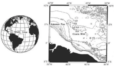
2.4. STUDY AREA

Ceara Rise, a seismic ridge currently situated 2600-3200 meters below

sea level,islocated intheAtlantic Ocean(Figure 3) some800kilometers eastof

theAmazonRiver,surroundedonthenorth,westandsouthbydistaldepositsfrom

Amazon Fan(HEINRICHetal.,2013).

Figure3.LocationofCearaRiseintheAtlanticOcean.AdaptedfromCURRYetal.,1994.

Some 80 million years ago, estimated time of origin of Ceara Rise

according tostudiesbytheageofigneous baseascension(SUPKOet al.,1977),

theregionwassubjectedtointensevolcanicextrusion,generatingfracturesupto2

km thick.ThisperiodwasmarkedbyfitsofplatesintheNorthandSouthAtlantic,

(26)

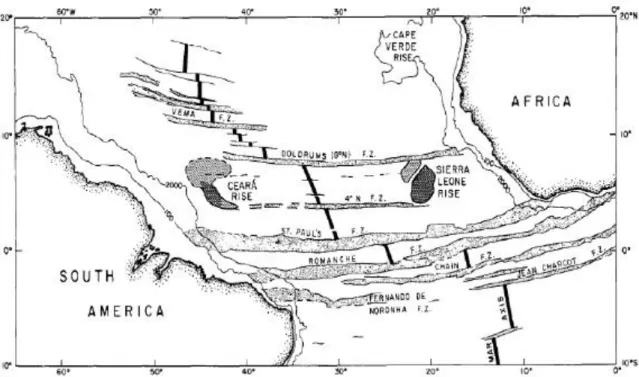
After the cessation of extrusive activity, the volcanic pile resulting from

suchseismic activitywasdividedintotwosegments(Figure4):theCearaRise,to

the west,andtheSierraLeoneRise,totheeast(KUMARetal.,1977).

Figure4.StructuralmapoftheequatorialAtlanticandoftheboundariesoftheCearaRiseand SierraLeoneRise,fromKUMARetal.,1977.

Since itsformation,thedepositionof limestoneandsiliceousmaterialhas

decreased the elevation of theCeara Rise.However, withthe growth of Amazon

FanintheEarlyMiocene,therewasalsotheintensificationofinfluxofterrigenous

material,whichisgreaterduringperiodsoflowsealevelandgeneratedaveryhigh

sedimentationintheregion(KUMARetal.,1977;HEINRICHetal.,2013).

Amazon Fanis abodyof sediments ofdeepsubmarine waterlocated on

the continental margins of Brazil and contains eroded material of the Amazon

Riverbasin.With sedimentsoriginatedfrom thisplaceitispossibletounderstand

the effect of climate changes that occurred during the Quaternary, because the

equatorialregionsplayedanimportantroleintransportingheattohighlatitudesin

(27)

presentinCearaRisecomesfromAmazon(KUMARetal.,1977),whichmakesit

able to monitor the changes that have occurred over the years in the region

(DOBSON etal.,2001).

This terrigenous material is usually deposited in the deepest parts of the

rise, which has distinctstratigraphic sequence due tothe deposition ofclays and

silts.InthehigherpartsoftheCearaRise,wherethesedimentationrateislow,the

main constitution of sedimentsis pelagic material, in other words, it comes from

theopensea(KUMARet al.,1977).

Therearealsocertainareasofhemipelagicssediments,consistingofboth

terrigenous and pelagic material. Thus, it is observed that the distribution of

sediments has large influence of deepwater’s movement (KUMAR et al., 1977).

ThedepthoftheseathatsurroundstheCearaRiseisapproximately4500meters

and surfacewatersshowlittleseasonalvariability(HEINRICHetal.,2013).

Therefore, the region is essential for understanding the dynamics of the

climatic phenomena occurred near the Amazon Fan, one of the largest modern

submarinefans (FLOODetal.,1997).

2.4.1. PREVIOUS WORK

ThepresentstudyisacontinuationoftheworkdevelopedbyDobson etal.

(2001) andotherresearchers, asCurryetal.(1995)and Murayamaet al.(1997),

who also studied and analyzed different properties of the samples collected in

CearaRise,site925.

TheworkofCurryetal.(1995)presentsadetaileddescriptionofsampling

performed at site 925, specifying the drilling techniques, the division of the core

into subparts and the relationship between depth and age of each sample,

(28)

presented data of percentage of carbonates, magnetic susceptibility

measurements, particle size and x-ray diffraction analyses, besides

lithostratigraphicdescription ofthesamples (AppendixB).

Murayamaetal.(1997)studiedsamplesfromsite925HoleB,toevaluate

the variation of 10Be,based on the rate of accumulation of sediments, to explain

the input of terrigenous material from the area of the Amazon drainage. They

concludedthattheratiobetween10Beand9Bewasnearlyconstantanddecreases

withdepth.Inaddition,10Beismainlyassociatedwithterrigenousfraction.

Subsequently, Dobson et al. (1997) performed chemical extractions to

isolate componentsand calculate the terrigenousmass accumulation ratesof 47

sediment samples from Ceara Rise. From the analysis of the elemental

composition, they observed both terrigenous material source and the rate of

accumulation of mass changed over the years, probably due to the influence of

Andeanupliftandtheincreaseoftheflowof theAmazonRiver.

In a following study, Dobson etal. (2001) evaluated the sources of river

discharge inSouth Americadescribing the rate of accumulation ofmass in other

57 coresediment samplesfromCearaRise.

Recently, Heinrich et al. (2013) studied the content of calcareous

dinoflagellate in sediment samples in Ceara Rise that corresponded to the

Neogene. The fossils of these species that develop in the oceans are able to

reflect the aquatic environment. They are also tools used for understanding the

oceanographicchanges,thedevelopmentoftheAmazonRiverandtheconditions

ofthewatersurfaceintheCearaRise,site926,wheretherewerelowacumulation

rates of calcareous dinoflagellates under 12 Ma and the subsequent increase

(29)

3. MATERIALS

AND

METHODS

3.1. SAMPLE COLLECTION AND PREPARATION

The sediments usedin this study areoriginated from the exploration site

925,onthetopoftheCearaRise(Figure5).Theexpeditiontookplacein1994and

the samples were collected by Curry et al. To ensure the completeness of

informationfromcoresamples,threeparallelholes(A,BandC)weremade,andin

thisstudytwoofthemareanalyzed,AandB.Thesamplesoriginatedfromthesite

925 A vary between 303 and 660 meters below seafloor (mbsf). However, the

samples fromsite925B varybetween zero and312mbsf.Theseintervals range

fromtheearlyOligocene(~30millionyearsago)tothepresentday(CURRYetal.,

1995). The depth and the corresponding age (Tables 1 and Table 2) for each

sample were obtained through the study of nannofossil (CURRY et al., 1995).

Information aboutholesAandBareshowninTable3.

(30)

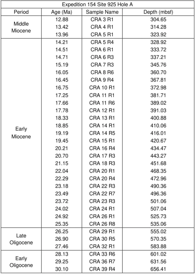
Table1.InformationabouttheCoreRecoveryA(CRA):period,age,sample´snameanddepth.

Expedition154Site925HoleA

Period Age(Ma) SampleName Depth(mbsf)

Middle Miocene

12.88 13.42 13.96

CRA3R1

CRA4R1

CRA5R1

304.65 314.28 323.92 Early Miocene 14.21 14.51 14.71 15.19 16.05 16.45 16.75 17.25 17.66 17.78 18.33 18.85 19.19 19.45 20.21 20.70 21.15 22.04 22.29 23.18 23.49 23.72 24.02 24.92 25.35

CRA5R4

CRA6R1

CRA6R3

CRA7R3

CRA8R6

CRA9R4

CRA10R1

CRA11R1

CRA11R6

CRA12R1

CRA13R1

CRA14R1

CRA14R5

CRA15R1

CRA16R4

CRA17R3

CRA18R3

CRA20R1

CRA20R4

CRA22R3

CRA22R7

CRA23R3

CRA24R1

CRA26R1

CRA26R8

328.92 333.72 337.21 345.76 360.70 367.81 372.98 381.71 389.02 391.03 400.88 410.06 416.01 420.67 434.47 443.27 451.68 468.35 472.96 490.36 496.36 501.06 507.04 525.73 535.06 Late Oligocene 26.25 26.90 27.46

CRA29R1

CRA30R5

CRA32R1

555.02 570.35 583.88 Early Oligocene 28.13 29.25 30.10

CRA33R6

CRA36R7

CRA39R4

(31)

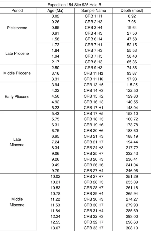
Table2.InformationabouttheCoreRecoveryB(CRB):period,age,sample´snameanddepth.

Expedition154Site925HoleB

Period Age(Ma) SampleName Depth(mbsf)

Pleistocene 0.02 0.26 0.65 0.91 1.58

CRB1H1

CRB2H3

CRB3H4

CRB4H3

CRB6H4

0.92 7.95 19.64 27.50 47.58 LatePliocene 1.73 1.84 1.94 2.17

CRB7H1

CRB7H3

CRB7H5

CRB8H3

52.15 55.53 58.40 65.36 MiddlePliocene 2.50 3.16 3.31

CRB9H3

CRB11H3

CRB11H6

74.86 93.87 97.93 EarlyPliocene 3.94 4.22 4.50 4.92 5.23

CRB13H5

CRB14H3

CRB15H2

CRB16H3

CRB17H1

115.25 122.50 129.80 140.55 148.04 Late Miocene 5.43 5.75 6.31 6.75 6.95 7.24 8.34 9.06 9.26 9.49 9.79

CRB17H5

CRB18H3

CRB19H6

CRB20H6

CRB21H3

CRB21H7

CRB24H3

CRB25H7

CRB26H3

CRB26H6

CRB27H4

153.10 160.72 173.78 183.60 188.19 194.44 217.72 232.43 236.41 241.04 246.96 Middle Miocene 10.02 10.21 10.53 10.78 11.22 11.53 11.84 12.24 12.55 13.07

CRB27H7

CRB28H3

CRB28H7

CRB29H4

CRB30H3

CRB30H7

CRB31H4

CRB32H3

CRB32H7

CRB33H7

(32)

Table3.Basicinformationofthestudiedexplorationcore.

CoreCode ODP154SITE925A ODP154SITE925B

Lat/long(°) 4°12.249N,43°29.334W 4°12.248N,43°29.349W

Enddepth(m) 930,4 318

Begindate 14thfebruary1994 8thfebruary1994

Enddate 19thfebruary1994 10thfebruary1994

Objective Studythehistoryofdeep-watercirculation

In total, 72 sediment samples were analyzed in the present work. The

samples werestoredinbagsat-18°Cuntillabanalyses.

3.2. ORGANIC GEOCHEMISTRY

3.2.1. CLEANING GLASSWARE

Initially, all glassware were washed with detergent and tap water. Then, the

materials werewashed withdeionizedwaterandmaintainedforatleastonenight

in a solution 2-5 % of Extran MA 02 in deionized water. Removed from the

detergent solution,the materials werewashed with deionized waterand dried in

an ovenat100°Cfor2hours.Finally,theopeningsoftherecipients weresealed

with aluminum foil.During laboratorywork, eachmaterial was washed twicewith

methanol(MeOH)andtwicewithdichloromethane(DCM)beforeuse

.

(33)

3.2.2.1. EXTRACTION OF ALKENONES AND

N-

ALKANES

For biomarker analysis, about 15 g of each sample was wrapped in

aluminum foil and freeze dried (Liotop L101) for 24 hours. After drying, the

samples were homogenized using a mortar and pestle until it formed a fine

powder.

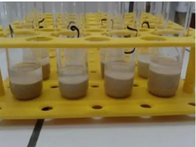
3 gofthehomogenizedsamplewereplacedincentrifugetubesand5mL

of DCM/MeOH (2/1) solution was added (Figure 6). The centrifuge tube was

placed in an ultrasonic bath (Cole-Parmer 8893) for 5 min and subsequently

centrifugedat300rpmfor5min(KindlyKCS).Thesupernatantwascollectedand

theextraction procedurewasrepeatedfourmoretimes.

Figure6.ExtractsofsedimentsamplesfromCearaRise.

The resulting total lipid extract (TLE) was evaporated on a rotary

evaporator (IKA RV 10 Basic) with heating bath at 30 °C. The final volume was

transferred to a previously weighed vial of 4 mL through a column containing

sodiumsulfate (Na2SO4)and cottonatthebottom(Figure 7)and thencompletely

(34)

TLE.100µLofeachinternalstandardsolution(scaleneandketone)wereaddedto

the TLEandtheextractwasdriedagain.Themethod usedwasadaptedfromthe

workofKimetal.(2009),followedbyvalidation.

A B

Figure7.(A)SodiumsulfatecolumnpreparedinaPasteurpipetteand(B)systemtotransferthe extracttothevialthroughthecolumn.

3.2.2.2. PREPARATION OF INTERNAL STANDARDS

The internal standardused foranalysis ofalkenones waspreparedusing

a solution of 2-nonadecanone in hexane. To prepare the solution, 10 mg of

2-nonadecanone wasweighed(ShimadzuModelAX200)inavialandsuccessive

dilutions weremadetoobtaintheconcentration of1µgmL-1.Theprocessfor the

preparation of solution of squalene in hexane (1 µg mL-1) used as internal

standardinthenonpolarfractionwasthesameusedforalkenones.

3.2.2.3. SEPARATION OF FRACTIONS OF ALKENONES AND

N-

ALKANES

To separatetheTLEinfractionscontaining n-alkanes,alkenonesandthe

(35)

the aluminum oxide was kept in an oven at 150 °C for 2 hours and placed in a

desiccator for 1hourwith desiccantagent. Toprepare thecolumn, it wasused a

smallpipettewithcottonatthebottomandapproximately4cmofaluminumoxide.

First,the TLEwasdiluted in2.5mLofhexane/DCM (9/1)andtransferred

to the column. The column was then washedtwice with 2.5 mL of hexane/DCM

(9/1)solution toelutethenonpolarfractionofTLE.

For separating the fraction corresponding to alkenones, the vial that

contained the extract was washed with a 2.5 mL of hexane/DCM (1/1) solution

three timesand transferred to a previously weighed vialof 1 mL using the same

columnusedforthenonpolarfraction.

To separate the fraction corresponding to polar compounds, the

procedure described above was repeated using 2.5 mL of DCM/MeOH (1/1)

solution.

Finally, the solvent of each fraction was completed evaporated using

nitrogen flow and themass of each fraction was determined. The scheme of the

(36)

Figure8.Generalschemeoftheanalyticalworkflow.

3.2.3. DETERMINATION AND QUANTIFICATION OF ALKENONES

The fractioncorrespondingtothe alkenoneswasanalyzed usingamodel

7890AGas ChromatographcoupledtoaFlameIonization Detector(GC-FIDfrom

Agilent Technologies). All samples were dissolved in 50 µL of hexane and

injected using an Agilent 7650A autosampler. The column used was a silica

capillary (phase DB-5, 25 m x 0.32 mm, film thickness 0.25 µm). The injected

sample volume was 1 µL and the column flow was 2.4 mL min-1, at constant

pressure.

The quantification ofalkenones wastaken inrelation tothe integration of

theareaunderthepeak.Theareaunderthepeakofalkenoneswasobtainedand

compared to the area under the peak of the internal standard. Each component

(37)

3.2.4. DETERMINATION AND QUANTIFICATION OF

N

-ALKANES

The fraction corresponding to the n-alkanes was analyzed by GC-FID

(same equipment used for alkenones quantification, Figure 9) and quantification

of n-alkanes was taken in relation to the integration of the area under the peak.

The area under the peak of n-alkanes was obtained and compared to the area

under thepeakoftheinternalstandard.

Additionally,ananalyticalcurvewasmade.Thiscurveservedasatoolfor

assessmenttheinternalstandard quantificationmethod.

For building the analytical curve, 1.1 mL of n-alkanes standard solution

(SupelcoAnalyticalC8-C40AlkanesCalibrationStd,500-5000µgmL-1inCH2Cl2)

was diluted to 10 mL of hexane. The eight points of the analytical curve was

constructed (0.055, 0.165, 0.33, 0.66, 1.1, 2.2, 4.4 and 5.5 µg mL-1) with

successive dilutionsofthe standard.

Thestandards usedtoconstructtheanalyticalcurvearelistedinTable 4.

Table4.Informationaboutthestandardusedtomaketheanalyticalcurve.

Register number

Numberofcarbon Name Concentration

(µgmL-1₎

629-97-0 22 N-Docosane 499.0

638-67-5 23 N-Tricosane 500.5

646-31-1 24 N-Tetracosane 501.0

629-99-2 25 N-Pentacosane 501.0

630-01-3 26 N-Hexacosane 500.5

593-49-7 27 N-Heptacosane 501.0

630-02-4 28 N-Octacosane 501.0

(38)

638-68-6 30 N-Triacontane 500.5

630-03-8 31 N-Hentriacontane 500.0

544-85-4 32 N-Dotriacontane 500.5

630-05-7 33 N-Tritriacontane 501.1

14167-59-0 34 N-Tetratriacontane 500.0

630-07-9 35 N-Pentatriancontane 500.1

Figure9.Gaschromatographywithflameionizationdetector(GC-FID)Agilent7650A.

Theparametersusedinthedeterminationofalkenonesandn-alkanesare

(39)

Table5.ChromatographicparametersoftheGC-FIDusedinthedeterminationofalkenonesand

n-alkanes.

Parameters Alkenonesmethod N-alkanesmethod

Injector

Column

Detector

Temperature(°C) Injectionmode Purgeflowtosplitvent

Carriergas

Temperatureprogramming

Pressure Totalruntime(min)

Temperature(°C)

Makeupgas

Flow(mLmin-1)

300 Splitless

40mLmin-1_at_0.5_min Helium

70 °C (hold time 0

min); 20 °C min-1

until200°C;3°Cmin-1 until 320 °C; 320 °C during25min

Constant 71 330 Nitrogen 24 300 Splitless

40mLmin-1_at_0.5_min Helium

70 °C (hold time 0

min);20°Cmin-1 until

130 °C; 4 °C min-1

until 320 °C; 320 °C

during30min

Constant 71 330 Nitrogen 24

3.3. VALIDATION

3.3.1. DETERMINATION OF OUTLIERS IN ANALYTICAL CURVES

Grubb'stest,knownasGtest,wasusedtoverifythepossiblepresenceof

outliers in the analytical curves. In this test, the sample standard deviation is

compared with thedeviation of thesuspected measured in relation tothe media,

accordingtoequation6:

(40)

Wherexisthevalueofthemeasure, istheaveragevalueandsisthestandard

deviation. If the calculated value of G is greater than the tabular value, the

measureisanoutlierandshouldbeexcludedfromtheline(MILLERetal.,2005).

3.3.2. LINEARITY

The analyticalcurvesforquantificationofn-alkanesweregeneratedfrom6points

intriplicate.Thelinearityofthesecurveswasevaluatedinrelationtoitscoefficient

correlation (R). According the National Institute of Metrology, Quality and

Technology(Inmetro),alinearrelationshipisobtainedforvaluesofRgreaterthan

0.90(Aragão,2009).

3.3.3. REPEATABILITY TEST

The precision of the analytical method was evaluated for repeatability.

According to recommendations of the Guide to International Conference on

Harmonisation (ICH) and the National Health Surveillance Agency (ANVISA)

ResolutionNumber899,thevalueofthenumericprecisionlevelofrepeatabilityis

estimated by the coefficient of variation (CV)of nine determinationscovering the

entire calibration range, with samples in triplicate (Equation 7) (RIBEIRO et al.,

2008).

CV= (7)

Solutions withexternalstandards of2-nonadecanoneand squalene were

used inthefollowingconcentrationlevelsforthistest:0.11,1.0e5µgL-1.

(41)

The t test for comparison of averages was used to assess whether the

concentration obtained using the internal standard method are statistically equal

tothevaluesof concentrationobtained fromtheexternalstandardmethod.

In this test, the valueof t-calculated is compared with the t-tabular value

for a normal distribution with g degrees of freedom. Ifthe calculated valueof t is

less than the tabular, it can be considered that the values are statistically equal.

Otherwise, the valuesare statistically different. Thecalculated value of t and the

number of g degrees of freedom are calculated, respectively, according to

equations8and9.

t= (8)

g= (9)

where and are,respectively,theaverageandthestandarddeviationofthe

concentration values calculatedfrom thecomparison withtheareaofthepattern,

and are the average and standard deviation of the concentration values

calculated from the analytical curves and and are the number of

replicatesforeachcase.

3.3.5. RECOVERY TESTS

Tests were performed to evaluate the recovery factor of the analytes in

thefollowingrespects:

a)Rotoevaporationandconcentrationwithaflowofnitrogen gas;

(42)

Sedimentsamplescollected atLakeParanoa (anartificial waterreservoir

located intheDistrito Federal,Brazil)wereusedtocarryouttherecoverytests.

For evaluation of the rotoevaporation step followed by concentration in

nitrogen gas, 100 µL of squalene solution (1mg mL-1) was added to 25 mL of

DCM/MeOH (2:1 v/v) and it was subjected to concentration steps. This solution

was analyzed by GC-FID and the results were compared with those obtained

whenthesolution isnotrotoevaporatedandconcentratedundernitrogenflow.

The same procedure described above was performed with respect to

alkenones,using100µLof2-nonadecanonesolution (1mgmL-1).

Finally, therecoverywascomparedwhenperformingdifferentnumbersof

extractions. Forthis step,the lakesediment was extractedfive (inthe same way

as coresamples), ten,fifteenandtwentytimes,andanalyzedbyGC-FID.

3.3.6. LIMITS OF DETECTION AND QUANTIFICATION

The limit of detection (LOD) is the lowest concentration of the analytical

which can be detected by the technique and can be determined from the visual

method.Inthismethod,analysisof sampleswithlowanalyteconcentrationswere

performed andtheLODisthelowestconcentrationthatresultsinapeakthatcan

beseen(RIBEIRO etal., 2008).

The quantificationlimitwastakenas thelowestconcentrationpointofthe

(43)

4. RESULTS

AND

DISCUSSION

4.1. METHOD VALIDATION

4.1.1. VERIFICATION OF OUTLIERS

Grubb's test was performed to identify possible outliers in the analytical

curves. TheG valuescalculated werecompared with thetabularvalue (P =0.05

of significance and G critic equal to 1.155). Since none of the calculated values

was greater than the critic value of G, it can be concluded that there were no

outliersinthecurvesandnovaluehasbeenrejected.

4.1.2. LINEARITY

The analytical curves were constructed from six points with different

concentrationsofn-alkanes,intriplicate.Thevaluesofthecorrelationcoefficients

obtainedareshowninTable6.

Table6.Valuesofcorrelationcoefficientsobtainedfromtheanalyticalcurves.

N-_alcane _R

N-Docosane 0.9973

N-Tricosane 0.9977

N-Tetracosane 0.9974

N-Pentacosane 0.9979

N-Hexacosane 0.9973

N-Heptacosane 0.9977

N-Octacosane 0.9978

(44)

N-Triacontane 0.9982

N-Hentriacontane 0.9978

N-Dotriacontane 0.9975

N-Tritriacontane 0.9977

N-Tetratriacontane 0.9974

N-Pentatriacontane 0.9963

AccordingtoInmetroallcurvescanbeconsidered linear.

4.1.3. REPEATABILITY

Therepeatabilitywasevaluatedtakingintoaccountthestandarddeviation

(SD)andcoefficientofvariation (CV).Solutionsofsqualene and2-nonadecanone

standardswereusedintriplicateatthreeconcentrationlevels:0.11,1.0and5.0µg

mL-1(Table).

Table7EstimationofSDandCVtothestandardsofsqualeneandnonadecanonethroughthe repeatabilityofareas(inpicoampere(pA)).

Concentration Area1 Area2 Area3 Average SD CV(%)

0.11µgmL-1 1.21 1.03 1.22 1.15 0.10 9.08

Squalene

2-Nonadecanone

1.0µg mL-1 8.17 8.08 8.50 8.25 0.22 2.71

5µgmL-1 52.97 46.09 48.09 49.05 3.54 7.22

0.11µgmL-1 1.01 1.01 1.06 1.03 0.03 2.75

1.0µg mL-1 7.95 9.18 10.11 9.08 1.09 11.95

5µgmL-1 55.23 36.66 49,.29 47.06 9.48 20.15

According Ribani et al. (2004) the maximum value for the coefficient of

(45)

the exception of alkenones with concentration equal 5 µg mL-1, the others

coefficients of variation are smaller than 12%, validating the method of

determination in trace level for n-alkanes and alkenones. None of the samples

showed alkenones concentrations equal to or higher than 5 µg mL-1 and it is

believed thatthehighcoefficientforthemostconcentratedsamplesisdueto loss

of linearitytheendsofacurve.

4.1.4. T TEST FOR COMPARISON OF CONCENTRATIONS

The test forcomparison ofvalues wasused to validate thequantification

performed from internal standard method. In this test, the values obtained from

the internal standard method were compared with the concentrations obtained

from the external standard method, taking in consideration the value of t

calculatedaccordingtoEquation8.

This test was performed for the following Samples: CRB 4-3H, CRB

14H-3, CRB 24H-3, CRB 30H-7 , CRA-1 and CRA 14R-1 and CRA 18 R-3

(46)

Table8.Valuesoft-calculatedfortheaveragecomparisontest.

t-calculated

Sample C-22 C-23 C-24 C-25 C-26 C-27 C-28 C-29 C-30 C-31 C-32 C-33 C-34 C-35

CRB3H-4 1.475 1.133 0.747 0.881 0.908 0.740 0.961 0.780 0.892 0.734 0.796 0.853 1.230 1.525 CRB14H-3 4.758 7.415 2.909 1.756 1.068 0.212 0.625 0.402 2.653 0.148 1.013 1.092 2.035 1.379 CRB24H-3 3.411 1.561 1.076 0.351 0.011 0.279 0.099 0.419 0.094 0.530 0.194 0.351 0.181 0.218 CRB30H-7 9.408 5.873 4.264 7.784 1.160 0.859 0.563 2.245 1.314 0.066 0.684 0.797 8.795 0.396

CRA14R-1 2.931 2.274 1.563 1.488 1.339 1.072 1.413 0.626 1.186 1.011 0.397 0.770 0.145 1.611

CRA18R-3 0.275 1.818 1.908 3.548 3.783 1.100 1.501 1.908 6.920 1.922 0.299 0.229 0.344 3.398

The number of degrees of freedom for the samples, calculated according to Equation 7, was 2. Comparing the T-calculated and the

respectivedegreeoffreedom withthet-tabulated value(9.925),itcanbeseenthatforallsamplesused inthistest,thevalueofthecalculated

concentration from the internal standard method is statistically equal to the concentrations calculated from the external standard method for

(47)

R e co v e ry fa ct o r( % )

4.1.5. RECOVERY TESTS

Therecoverymethodwasevaluatedintermsoftheconcentration step

andforthecompletemethod.

Toevaluatethestageofrotoevaporationandconcentrationwithflowof

nitrogen gas, solutions with squalene (1mgmL-1) and 2-nonadecanone (1mg

mL-1)standardswereused.Therecoveryfactorforalkenones andn-alkanes is

showninFigure 10.

120 100 110,0 80 60 40 20 0 63,0 Alkenones N-alcanes Compounds evaluated

Figure10.Recoveryfactors(%)ofrotoevaporationandconcentrationstepsofthesolventwitha nitrogenflow.

To assess the recovery factor of the complete method, superficial

sediment samples from Lake Paranoa were extracted in ultrasonic bath five

times (as the method used for all the samples), ten, fifteen and twenty times.

(48)

Co n ce n tr ati o n (u g m L -1 ) Co n ce n tr ati o n (u g m L -1 )

Alkenones

7 6 5 4 3 2 1 0

Five extractions Ten extractions Fifteen extractions Twenty extractions

Number of extractions

Figure11. Comparingtheconcentrationsobtainedfordifferentnumberofextractionsofalkenones.

N

_-alkanes

90 80 70 60 50 40 30 20 10 0

Five extractions Ten extractions Fifteen extractions Twenty extractions

Number of extractions

Figure12.Comparingtheconcentrationsobtainedfordifferentnumberofextractionsofn-alkanes.

When five extractions were performed, the concentration of extracted

(49)

highest concentration extracted. For alkenones, the best result was obtained

whentheextraction wasperformedtentimesand,forn-alkanes,fifteentimes.

Afterreachingthemaximum,theconcentrationofanalyteintheextract

decreases,probablyduetotheextensivetimerequiredofrotoevaporationtoget

thevolumeof1mL.

ItcanbeseenbycomparingFigure11and12thattheconcentrationsof

alkenones obtained in the recoverytest are lower than those obtainedfor the

n-alkanes. This can be explained by the fact that there was Unresolved

Complex Mixture (UCM) in the chromatograms offraction of ketonesand also

bytheabsenceofalkenonesobjectsofstudyinParanoaLakesamples.Thisis

becausethesedimentscollectedinthelakeareshallowandprobablytherewas

notenoughtimeforalkenonesweredeposited inthematrix.

4.1.6. LIMITS OF DETECTION AND QUANTIFICATION

TheLOD,obtainedbythevisualmethod,andtheLOQobtainedforthe

squaleneand2-nonadecanonestandardsareshowninTable9.

Table9.LODandLOQobtainedfornonadecanoneandsqualene.

Parameter LOD(µgmL-1) LOQ(µgmL-1)

2-nonadecanone 0.0313

-Squalene 0.0181 0.055

4.2. QUALITATIVE DETERMINATION OF

N-

ALKANES

The qualitative determination of n-alkanes was made from the

correlation of retention time of aliphatic hydrocarbons present in the standard

(50)

The retention times(RT) of n-alkanes usedfor this comparison andto

constructtheanalytical curvesareshowninTable10.

Table2.Retentiontimes(min)ofn-alkanesusedintheconstructionofanalyticalcurves

N-_alcane _Code _RT_(in_minutes)

N-Docosane C-22 34.1

N-Tricosane C-23 36.4

N-Tetracosane C-24 38.6

N-Pentacosane C-25 40.7

N-Hexacosane C-26 42.8

N-Heptacosane C-27 44.8

N-Octacosane C-28 46.7

N-Nonacosane C-29 48.6

N-Triacontane C-30 50.4

N-Hentriacontane C-31 52.2

N-Dotriacontane C-32 54.2

N-Tritriacontane C-33 56.3

N-Tetratriacontane C-34 58.6

N-Pentatriacontane C-35 61.3

Thesamplesshowchromatographicprofilesimilartothatobtainedfor

(51)

Figure11.Typicalchromatogramobtainedforn-alkanesextracts(sampleCRA5R4).

The other chromatograms obtained for the nonpolar fractions of the

(52)

Table11.Concentrations(µgmL )andtotalareasoftheexternalstandardanalyticalcurveofn-alkanesused.

(µgmL )

4.3. QUANTITATIVE DETERMINATION OF

N-

ALKANES

Analyticalcurveswereconstructedfromn-alkanespresentintheexternalstandard.Thecurves(Figure14to27)wereplottedusingthe

referent areas of each n-alkane (dependent variable) versus the known concentrations (independent variable) from 8 standard solutions

preparedfromdilutingthestocksolution (Table11).

-1

Averagearea(pA)

Concentration

-1 C-22 C-23 C-24 C-25 C-26 C-27 C-28 C-29 C-30 C-31 C-32 C-33 C-34 C-35

0.055 1.2 1.2 1.2 2.0 1.2 1.1 1.5 1.1 1.5 1.1 1.2 1.0 1.1 1.2

0.165 3.1 3.1 2.9 4.5 3.1 2.7 3.2 2.9 3.1 2.6 2.9 2.7 2.7 2.4

0.33 5.8 5.9 5.8 6.7 6.0 5.6 6.1 5.6 5.9 5.4 5.9 5.5 5.6 5.9

0.66 11.5 11.6 11.4 12.2 12.3 11.0 12.2 11.7 12.6 10.9 11.6 11.4 11.6 13.2

1.1 23.3 23.5 23.5 24.8 24.5 22.7 23.7 23.4 23.4 22.7 23.0 23.1 23.3 23.3

2.2 34.2 34.9 34.8 37.2 35.4 34.6 35.3 35.1 37.2 34.0 34.6 34.9 34.8 38.7

4.4 65.0 66.5 66.5 70.1 67.7 65.8 67.7 66.9 69.2 65.5 66.1 67.4 67.2 66.9

(53)

Ar ea (p A) Ar ea (p A) Ar ea (p A) Ar ea (p A) Ar ea (p A) Ar ea (p A) 90 80 70 60 50 40 30 20 10 0

0 1 2 3 4 5 6

90 80 70 60 50 40 30 20 10 0

0 1 2 3 4 5 6

Concetraction(µgmL-1₎

Figure12.AnalyticalcurveofC-22.

90 80 70 60 50 40 30 20 10 0

0 1 2 3 4 5 6

Concentraction(µgmL-1₎

90 80 70 60 50 40 30 20 10 0

0 1 2 3 4 5 6

Figure15.AnalyticalcurveC-25.

90 80 70 60 50 40 30 20 10 0

0 1 2 3 4 5 6 Concentraction(µgmL-1₎

90 80 70 60 50 40 30 20 10 0

0 1 2 3 4 5 6 Concentraction(µg/ml)

(54)

Ar ea (p A) Ar ea (p A) Ar ea (p A) Ar ea (p A) Ar ea (p A) Ar ea (p A) 90 80 70 60 50 40 30 20 10 0

0 1 2 3 4 5 6

90 80 70 60 50 40 30 20 10 0

0 1 2 3 4 5 6

90 80 70 60 50

90 80 70 60 50 40 30 20 10 0

0 0,5 1 1,5 2 2,5 3 3,5 4 4,5 5 5,5 6 Concentraction(µgmL-1

40 30 20 10 0

100 90 80 70 60 50 40 30 20 10 0

0 1 2 3 4 5 6

90 80 70 60 50 40 30 20 10 0

(55)

Ar ea (p A) Ar ea (p A)

Table12.EquationslinesandR foreachn-alkane.

90 80 70 60 50 40 30 20 10 0 90 80 70 60 50 40 30 20 10 0

0 1 2 3 4 5 6

Concentraction(µgmL-1_l)

Figure19.AnalyticalcurveofC-34. Figure20.AnalyticalcurveofC-35.

Theequationsofthelinesofeachrespectiven-alkaneandRare

showninTable12.

2

Equationline R

C-22 y=14.485+2.1032 0.9973 C-23 y=14.836+2.0247 0.9977 C-24 y=14.836+1.9342 0.9974 C-25 y=15.653+2.6065 0.9979

C-26 y=14.992+2.320 0.9973

C-27 y=14.67+1.7372 0.9977

(56)

The areas were obtained from the integration of the peaks and

interpolatedintheequationsofthelinesfor theexternal standardmethod.The

resulting concentration (in µg mL-1) was divided by the mass of each sample

multiplied by the volume present in each vial (50 µL) extract to give a final

concentrationinµgg-1ofsediment (Table13).

Fortheinternal standardmethod, theconcentrationswere obtainedby

the comparison with the area of the standard squalene. In this quantification

method,the areaof squalene, whoseconcentration inthe sampleisknown, is

(57)

Table3.Weightandsedimentconcentrations(µgg-1)of14n-alkanesinthesedimentsamplesofthecoresCRAandCRBofCearaRiseobtainedbyinterpolationintheanalyticalcurves.

Concentration(inµgg-1)

Weight

Sample C-22 C-23 C-24 C-25 C-26 C-27 C-28 C-29 C-30 C-31 C-32 C-33 C-34 C-35 (ing)

CRB-1H-1 2.02 <0 0.0385 0.0230 0.0415 0.0218 0.0524 0.0164 0.1119 0.0240 0.1173 0.0194 0.0575 <0 0.0159

CRB-2H-3 3.09 0.0562 0.0784 0.0581 <0 <0 0.0801 OLR OLR OLR OLR OLR 0.0792 OLR OLR

CRB-3H-4 3.11 0.0111 0.0177 0.0259 0.0566 0.0752 OLR OLR OLR OLR OLR 0.0644 OLR 0.0279 0.0261

CRB-4H-3 3.13 0.0013 0.0039 0.0050 0.0115 0.0188 0.0355 0.0394 0.0708 0.0418 0.0746 0.0256 0.0376 0.0093 0.0103

CRB-6H-4 3.17 OLR <0 OLR <0 OLR <0 OLR OLR OLR OLR OLR OLR OLR OLR

CRB-7H-1 3.12 0.0237 0.0161 0.0160 0.0325 0.0293 0.0330 OLR OLR 0.0257 OLR 0.0123 OLR 0.0123 0.0322

CRB-7H-3 3.20 0.0042 0.0080 0.0099 0.0196 0.0235 0.0540 0.0346 OLR 0.0424 OLR 0.0311 OLR 0.0114 0.0255

CRB-7H-5 3.07 0.0033 0.0063 0.0074 0.0166 0.0220 0.0373 0.0343 0.0830 0.0378 0.0836 0.0265 0.0530 0.0100 0.0176

CRB-8H-3 3.17 0.0024 0.0065 0.0082 0.0186 0.0208 0.0452 0.0264 0.0808 0.0296 OLR 0.0190 0.0779 0.0078 0.0193

CRB-9H-3 3.16 0.0010 0.0039 0.0039 0.0094 0.0141 0.0225 0.0196 0.0458 0.0244 0.0526 0.0169 0.0316 0.0075 0.0091

CRB-11H-3 3.02 0.0053 0.0081 0.0125 0.0209 0.0317 0.0393 0.0407 0.0691 0.0674 0.0736 0.0479 0.0429 0.0268 0.0185

CRB-11H-6 3.14 OLR OLR 0.0717 OLR OLR <0 OLR OLR OLR OLR OLR <0 OLR OLR

CRB-13H-5 3.00 0.0086 0.0188 0.0232 0.0350 0.0492 0.0531 0.0568 0.0904 0.0606 0.0811 0.0479 0.0473 0.0274 0.0183

CRB-14H-3 3.06 0.0020 0.0053 0.0097 0.0174 0.0294 0.0383 0.0383 0.0611 0.0387 0.0613 0.0254 0.0324 0.0113 0.0103

CRB-15H-2 2.92 <0 <0 <0 OLR 0.0021 0.0054 0.0062 0.0113 0.0084 0.0134 0.0049 0.0066 0.0008 0.0015

(58)

57

CRB-17H-1 3.00 OLR OLR 0.0013 0.0049 0.0162 0.0362 0.0498 0.0776 0.0552 0.0704 0.0322 0.0352 0.0142 0.0073

CRB-17H-5 2.04 0.0034 0.0081 0.0097 0.0131 0.0156 0.0302 0.0207 0.0776 0.0262 0.1297 0.0186 0.0913 0.0066 0.0231

CRB-18H-3 3.19 OLR OLR OLR <0 OLR OLR OLR OLR OLR 0.0608 OLR <0 OLR OLR

CRB-19H-6 3.10 OLR OLR OLR <0 OLR OLR OLR OLR OLR 0.0383 OLR <0 OLR OLR

CRB-20H-6 2.93 OLR OLR OLR <0 OLR OLR OLR 0.0859 OLR 0.0488 OLR <0 0.0875 0.0703

CRB-21H-3 3.19 0.0051 0.0151 0.0110 0.0140 0.0210 0.0434 0.0303 OLR 0.0371 OLR 0.0240 0.0601 0.0095 0.0184

CRB-21H-7 3.19 0.0014 0.0036 0.0091 0.0170 0.0315 0.0367 0.0393 0.0508 0.0425 0.0551 0.0333 0.0306 0.0179 0.0138

CRB-24H-3 3.04 <0 0.0018 0.0023 0.0062 0.0105 0.0133 0.0138 0.0302 0.0166 0.0423 0.0115 0.0224 0.0157 0.0062

CRB-25H-7 3.09 0.0011 0.0030 0.0038 0.0079 0.0169 0.0177 0.0178 0.0337 0.0277 0.0383 0.0194 0.0190 0.0102 0.0060

CRB-26H-3 3.14 OLR <0 OLR <0 OLR OLR OLR OLR OLR <0 OLR <0 OLR OLR

CRB-26H-6 3.06 OLR <0 OLR <0 OLR <0 OLR OLR OLR OLR OLR OLR OLR OLR

CRB-27H-4 2.90 0.0011 0.0093 0.0077 0.0145 0.0224 0.0220 0.0250 0.0530 0.0352 0.0718 0.0303 0.0507 0.0178 0.0175

CRB-27H-7 3.03 <0 OLR 0.0019 0.0045 0.0080 0.0098 0.0108 0.0155 0.0094 0.0140 0.0054 0.0071 0.0015 <0

CRB-28H-3 3.05 0.0448 <0 0.0436 <0 0.0146 0.0246 0.0218 0.0396 0.0554 0.0456 0.0330 0.0236 0.0210 <0

CRB-28H-7 3.10 0.0123 <0 <0 0.0060 0.0038 0.0173 0.0181 0.0309 0.0315 0.0367 0.0163 0.0178 <0 <0

CRB-29H-4 3.15 0.0239 0.0025 0.0258 0.0096 0.0209 0.0185 0.0185 0.0341 0.0332 0.0283 0.0192 0.0150 0.0086 <0

CRB-30H-3 3.10 0.0019 0.0046 0.0067 0.0100 0.0156 0.0220 0.0166 0.0481 0.0384 <0 0.0209 0.0212 0.0110 0.0178

CRB-30H-7 3.04 0.0010 0.0077 0.0197 0.0362 0.0590 0.0689 0.0737 OLR 0.0762 0.0845 0.0559 0.0474 0.0277 0.0245

CRB-31H-4 3.00 OLR 0.0032 0.0044 0.0100 0.0155 0.0183 0.0192 0.0307 0.0234 0.0305 0.0169 0.0152 0.0059 0.0039