Recurrent frequency-size distribution of characteristic events

(1)

www.nonlin-processes-geophys.net/16/333/2009/ © Author(s) 2009. This work is distributed under

the Creative Commons Attribution 3.0 License.

in Geophysics

Recurrent frequency-size distribution of characteristic events

S. G. Abaimov1, K. F. Tiampo1, D. L. Turcotte2, and J. B. Rundle2

1_{Department of Earth Sciences, University of Western Ontario, London, Canada} 2_{Department of Geology, University of California, Davis, USA}

Received: 24 October 2008 – Revised: 31 March 2009 – Accepted: 3 April 2009 – Published: 28 April 2009

Abstract. Statistical frequency-size (frequency-magnitude) properties of earthquake occurrence play an important role in seismic hazard assessments. The behavior of earthquakes is represented by two different statistics: interoccurrent be-havior in a region and recurrent bebe-havior at a given point on a fault (or at a given fault). The interoccurrent frequency-size behavior has been investigated by many authors and generally obeys the power-law Gutenberg-Richter distribu-tion to a good approximadistribu-tion. It is expected that the recur-rent frequency-size behavior should obey differecur-rent statistics. However, this problem has received little attention because historic earthquake sequences do not contain enough events to reconstruct the necessary statistics. To overcome this lack of data, this paper investigates the recurrent frequency-size behavior for several problems. First, the sequences of creep events on a creeping section of the San Andreas fault are investigated. The applicability of the Brownian passage-time, lognormal, and Weibull distributions to the re-current frequency-size statistics of slip events is tested and the Weibull distribution is found to be the best-fit distribu-tion. To verify this result the behaviors of numerical slider-block and sand-pile models are investigated and the Weibull distribution is confirmed as the applicable distribution for these models as well. Exponents β of the best-fit Weibull distributions for the observed creep event sequences and for the slider-block model are found to have similar values rang-ing from 1.6 to 2.2 with the correspondrang-ing aperiodicitiesCV of the applied distribution ranging from 0.47 to 0.64. We also note similarities between recurrent time-interval statis-tics and recurrent frequency-size statisstatis-tics.

Correspondence to:S. G. Abaimov (sgabaimov@gmail.com)

1 Introduction

The statistics of earthquake occurrence exhibit two types of behavior. In this paper we will follow the terminology in-troduced by Abaimov et al. 2007b). The term “interoccur-rent”(or“interoccurrence”) refers to earthquake sequences on all faults in a region. The term“recurrent”(or “recur-rence”) refers to earthquake sequences on a single fault or fault segment. Earthquakes will be referred to as character-isticearthquakes if they have approximately the same rupture area equivalent to the area of the fault or fault segment. More specifically, the probability density function (pdf) of areas must have a well-defined maximum and a coefficient of vari-ation in the range 0.3 to 0.7. Two examples of characteristic earthquakes are the sequence of large earthquakes that have occurred on the Parkfield section of the San Andreas fault in California (Bakun et al., 2005) and the sequence of great earthquakes that have occurred on the southern section of the San Andreas fault (Biasi et al., 2005).

An important aspect of earthquake behavior concerns the statistical properties of time intervals between successive earthquakes. We refer to these as thetime-interval statis-tics. Another important aspect of earthquake occurrence is the distribution of earthquake sizes (magnitudes). We refer to these as thefrequency-sizestatistics. This paper investi-gates therecurrent frequency-sizestatistics ofcharacteristic

earthquakeson a fault(orfault segment) orat a given point on a fault. We will be primarily concerned with the slip am-plitudesS.

(2)

was also found for simulations of the slider-block model (Carlson and Langer, 1989), and for the sand-pile model (Bak et al., 1988).

Alternative measures of the size of an event are avail-able. Earthquake size can be measured not only by the earth-quake’s emitted energy or seismic moment, but also by the average slip amplitude. The energy of an eventEhas a power law dependence on the average slip amplitudeS

E_∝Sδ (1)

whereδ is typically equal to 3 (Kanamori and Anderson, 1975). Gutenberg-Richter power law dependence is invariant to power law transformations. Therefore Gutenberg-Richter power law statistics for a region are valid not only for the energy distributions but also for the frequency-amplitude distributions.

However, knowledge of only interoccurrent properties is often not sufficient to inherently improve seismic hazard es-timations. It is also necessary to know the statistical prop-erties of another type of behavior – therecurrent behavior at a given point on a fault or on a given fault. Unfortu-nately, there is much less information available on this type of behavior. The reason for this is that this type of behav-ior is much more difficult to investigate (Savage, 1994). For the interoccurrent frequency-size statistics of a region it is only necessary to count magnitudes of earthquakes that have occurred in this region. For the recurrent behavior it is re-quired to associate these earthquakes with a specific fault or fault segment. As a result, the question of which statistics correspond to the recurrent behavior of earthquakes remains controversial. In addition, while the recurrent time-interval statistics have been investigated by many authors (Abaimov et al., 2007a, b; Matthews et al., 2002; Molchan, 1990, 1991; Nishenko and Buland, 1987; Rikitake, 1982; Utsu, 1984), only a few attempts have been made to investigate the re-current frequency-sizestatistics (e.g., Abaimov et al., 2007a; Bakun et al., 2005).

This paper focuses on investigating the recurrent frequency-size statistics of characteristic earthquakes on a fault or at a given point on a fault. As a specific example we will consider the recurrent frequency-size statistics of creep events on a creeping section of the San Andreas fault. We previously carried out a detailed study of the recurrent time-interval statistics of these events (Abaimov et al., 2007a). We will note the strong similarities between time-interval and frequency size statistics for these events. Because of this similarity we will apply the same trial distributions in this paper for the frequency-size distributions that we previously applied to the time-interval distributions. For this reason we consider the Weibull, Brownian passage-time, and lognormal distributions. It can be argued that the Weibull distribution (also known as the Rosin-Rammler distribution) is the pre-ferred distribution since it is widely applied to both time in-terval statistics, i.e. earthquakes, and to frequency-size

statis-tics, i.e. fragments. We will conclude that the Weibull distri-bution is in fact the preferred trial distridistri-bution.

If there were no fault complexity and displacements were applied to a fault at a constant rate, then the statistics of re-current time-intervals and sizes would be identical. However, this would imply the applicability of the time-predictable or slip-predictable models (Shimazaki and Nakata, 1980). Abaimov et al. (2007a) studied the applicability of these models to the recurrent slip events on the San Andreas fault and found no well defined predictability. However, the simi-larities in the distributions of time-intervals and sizes demon-strated in this paper are striking.

In Appendix A we briefly describe these distributions. The measures of goodness-of-fit that we use to evaluate the appli-cability of these distributions are described in Appendix B. These include the Kolmogorov-Smirnov test, the root-mean-squared error test, and visual inspection.

Ideally, observed sequences of earthquakes on a fault would be used to establish the applicable statistical distribu-tion. However, the numbers of events in observed earthquake recurrent sequences are not sufficient to establish the validity of a particular distribution (Savage, 1994). To illustrate this, in Sect. 2 we will consider the sequence of earthquakes on the Parkfield segment of the San Andreas fault.

In Sect. 3 of this paper we study sequences with a large number of recurrent events. For this purpose we investigate a creeping section of the San Andreas fault. Creep events on the central section of the San Andreas fault have been studied extensively. Creep measurements have been carried out since the 1960s by US Geological Survey and show both steady-state creep and well defined slip events (Langbein, 2004; Schulz et al., 1982, 1983; Schulz, 1989). We consider the recurrent statistics of slip events that are superimposed on the steady-state creep. In this case, we have enough events to differentiate among alternative proposed distributions. In each case we compare the data (sample distribution) with the three trial distributions and provide tests of goodness-of-fit.

Although the creep records provide enough (up to 100) events in a sequence to differentiate among the alternative trial distributions, we extend our testing with the aid of nu-merical simulations. A slider-block model is often used to study earthquake behavior on a given fault (see e.g. Abaimov et al., 2007b; Abaimov et al., 2008; Carlson and Langer, 1989). Therefore, in Sect. 4 we investigate the recurrent be-havior of the stiff slider-block model.

(3)

2 Parkfield sequence

Ideally, recurrent sequences of earthquakes would be used to establish a preferred statistical distribution. Unfortu-nately, the number of earthquakes available through histori-cal records is generally too small for adequate statistihistori-cal test-ing.

As an example we consider the sequence of seven char-acteristic earthquakes that occurred on the Parkfield (Cal-ifornia) section of the San Andreas fault between 1857 and 2004 (Bakun et al., 2005). The slip rate is quite high (_≈30 mm/year) and the earthquake magnitudes are rel-atively small (m_≈6.0), thus the recurrent times are short (_≈25 years). Also, this fault is subject to a nearly constant driving velocity due to the relative motion between the Pa-cific and North American plates. Earthquakes on the Park-field section of the San Andreas fault occurred in 1881, 1901, 1922, 1934, 1966, and 2004 with magnitudes ranging be-tween 6.0 and 6.05 from instrumental estimates and from 5.9 to 6.1 using the modified Mercalli intensity for an epicenter location on the 2004 rupture (Bakun et al., 2005). For the size of an event here we use the seismic moment or energy of this event.

However, the small number of registered earthquakes makes the application of statistical estimations impossible (Savage, 1994). And this problem is relevant not only for the Parkfield sequence. Other earthquake sequences are also similarly short (e.g., Okada et al., 2003; Park and Mori, 2007). Studying sequences of smaller events also has intrin-sic difficulties. Although smaller earthquakes have shorter periods of recurrence, another problem appears when one at-tempts to reconstruct the associated recurrent statistics on a particular fault. In other words, while for large magni-tude earthquakes, like the Parkfield sequence, it is possible to associate the events with a particular fault, the sequences are short. In contrast, for small magnitude earthquakes it is generally impossible to reconstruct the recurrent statistics due to the difficulty of associating the earthquake waveform with the rupture of a particular fault or fault segment. Even nearby locations and waveforms could belong to different faults for small magnitude earthquakes. And, vice versa, dif-ferent waveforms can be generated by the same fault. There-fore it is impossible to solve the problem using only historic recorded earthquake sequences.

The sequence of Parkfield earthquakes does, however, give a suggestion that the actual recurrent frequency-size distri-bution of characteristic events is much more repetitive (has a much lower aperiodicity) than the interoccurrent power-law Gutenberg-Richter distribution. Indeed, it is difficult to as-sociate the almost repetitive magnitudes (in the range from 5.9 to 6.1) of the Parkfield sequence with the scale-invariant, power-law Gutenberg-Richter distribution. In fact, exactly repetitive distribution (δ-function, all magnitudes are equal) is often used in probabilistic seismic hazard assessments. Is the recurrent frequency-size distribution of characteristic

events indeed exactly repetitive? Do earthquake magnitudes have no variability? Is there an actual statistical distribution that should be used instead of the δ-function? This paper examines these questions.

3 Slip events on a creeping section of the San Andreas fault

We now consider the recurrent statistics of slip events on the creeping section of the San Andreas fault in California. To do this we utilize records from two creepmeters on the San Andreas fault (Schulz, 1989). One of these is located near the Cienega Winery, 16.9 km southeast of San Juan Bautista (station “cwn1”, latitude 36◦45.0′, longitude 121◦23.1′). The creep measurements have been recorded since June 1972 by the US Geological Survey (USGS), and show that the aver-age long-term creep rate is about 11.5 mm/year. The second creepmeter is located near Harris Ranch, 12.8 km southeast of San Juan Bautista, and 4.1 km northwest from cwn1 (sta-tion “xhr2”, latitude 36◦_46.3′_{, longitude 121}◦_25.3′_{). These}

creep measurements have been recorded by the USGS since April 1985, and show that the average long-term creep rate is in the range of 6 to 9 mm/year. The recorded data for both creepmeters can be downloaded from the USGS web site (Langbein, 2004).

Each creep record provides a unique opportunity to deter-mine the complete sequence of events taking place at a given creepmeter location. In contrast to earthquakes, the rate of occurrence for creep events is much higher. Also each ob-served sequence of creep events provides a complete record of all events which occurred at a given location. This pro-vides an opportunity to associate events not only with the given fault but also with a given point of this fault. There-fore the reconstruction of event sequences from creep records gives both the longest possible sequences (up to 100 events) and the most accurate determination of the location of recur-rent events.

For both creepmeters the data contain both daily and 10 min telemetry records. Although there are longer se-quences of daily records, the 10 min data also are used inde-pendently because they provide more accurate slip amplitude resolution. Details of our investigation of the creep events have been given in our previous publication (Abaimov et al., 2007a). The recurrent time-interval statistics were studied in detail. In this paper we carry out a similar analysis of the recurrent frequency-size statistics.

(4)

(a)

0 1 2 3 4 5 6 7 8 9

0 20 40 60 80

xhr2 10 minute record

Cumulative number of events,

N

(

S

≥

S0

)

Slip amplitude S

0, mm (b)

0 1 2 3 4 5 6 7 8 9 10

0 20 40 60

cwn1 10 minute record

N

(

S

≥

S0

)

Slip amplitude S 0, mm

(c)

0 1 2 3 4 5 6 7 8 9

0 20 40 60 80

xhr2 daily record

N

(

S

≥

S0

)

Slip amplitude S

0, mm (d)

0 1 2 3 4 5 6 7 8 9 10

0 20 40 60 80 100 120

cwn1 daily record

N

(

S

≥

S0

)

Slip amplitude S

0, mm

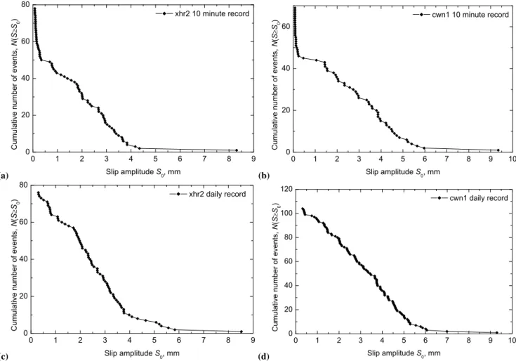
Fig. 1. Recurrent creep events (at a given point on a fault): cumulative number of slip events greater thanS0,N (S≥S0), versus the slip

amplitude,S0, for the(a)xhr2 10 min record,(b)cwn1 10 min record,(c)xhr2 daily record, and(d)cwn1 daily record. The cumulative

distribution functions are integrated from large to small amplitudes and are not normalized (similar to the Gutenberg-Richter distribution except only linear scales for both axes).

a stationary creeping state before the next jump, these two jumps are treated as separate. Otherwise, if one jump trig-gers another one in a transient, non-stationary process, these jumps are considered to be a single event.

Of course, there is a possibility that one independent event can occur shortly after another while the creep record is still in the non-stationary regime. For this case we would miss the real independent event. The same problem holds for a system with discrete events such as earthquakes when it is not possible to distinguish among aftershocks just immedi-ately after a mainshock. For the creep events the situation is even worse as sometimes the duration of an event can be comparable with the interval between events. In the creep records there are eight suspicious event occurrences (of the total 104 number of events) for the cwn1 daily record and four suspicious events (of the total 76 events) for the xhr2 daily record. Although this error can disturb the statistics we see that it is about 8% or less and therefore can be neglected. However, one important consequence is that this error can

produce outliers when amplitudes of several events are com-bined into one. In fact, we see one of these comcom-bined outliers with the amplitude about 9 mm in Fig. 1.

To filter the telemetry noise, threshold levels for slip am-plitude are used: 0.077 mm for 10 min xhr2 telemetry, 0.078 mm for 10 min cwn1 telemetry, 0.3 mm for xhr2 daily telemetry, and 0.31 mm for cwn1 daily telemetry. These thresholds are chosen to be as low as possible. For the ampli-tudes below these thresholds it is not possible to distinguish individual creep events from the noise in the signal.

(5)

Table 1.Creep event sequences: The recurrent slip amplitude statistics at a given point on a fault. For all sequences the parameters of the best-fit Brownian passage-time, lognormal, and Weibull distributions are given as well as the goodness-of-fit estimators.

Sequence Data or fit Data or fit parametersa Goodness-of-fit estimators

D_KS Q_KS Cdf

RMSE

Weibull plot RMSE

xhr2 10 min 51 events

Sample distribution µ=2.4 mm CV=0.56 Not applicable

Brownian passage-time µ=2.4±0.2 mm CV=0.72±0.08 0.18 0.07 0.09 0.3

Lognormal y=0.71¯ ±0.09b σy=0.65±0.06b

(CV=0.72±0.09)

0.14 0.2 0.07 0.2

Weibull τ=2.7±0.2 mm β=1.9±0.2

(CV=0.55±0.05)

0.09 0.8 0.04 0.09

cwn1 10 min 45 events

Lognormal y=1.10¯ ±0.08b σy=0.55±0.06b

(CV=0.59±0.07)

0.13 0.4 0.06 0.3

Weibull τ=3.9_±0.3 mm β=2.2_±0.2

(CV=0.47±0.05)

0.07 0.97 0.03 0.08

xhr2 daily 76 events

Lognormal y=0.73_¯ _±0.08b σy=0.73±0.06b

(CV=0.83±0.09)

0.15 0.07 0.07 0.19

Weibull τ=2.9_±0.2 mm β=1.78_±0.16

(CV=0.58±0.05)

0.08 0.7 0.04 0.09

cwn1 daily 104 events

Lognormal y=0.98_¯ _±0.07b σy=0.70±0.05b

(CV=0.80±0.07)

0.13 0.05 0.07 0.3

Weibull τ=3.63±0.19 mm β=2.00±0.16

(CV=0.52±0.04)

0.10 0.3 0.04 0.12

a_{The error bars are 95% confidence limits.}b_{Units of data in mm.}

characteristic events we impose an amplitude threshold of 0.3 mm and discard small amplitude events below this thresh-old. This approach appears to be reasonable. Indeed, the peak of non-characteristic events is narrow therefore its re-moval does not influence the statistics of the remaining char-acteristic events significantly.

The discussion above seems to be ambiguous because it appears as if we are removing the peak of small ampli-tudes only because it does not follow the ‘smooth’ curve of statistics and because we attribute these events to be non-characteristic. The difficulty here, as for the case of earth-quakes, is that we cannot determine the real extension of the rupture of an event under Earth’s surface. Therefore we do not have a specific, detailed criterion for the separation of characteristic events. The technique, described above, is in fact inspired by the numerical simulations of the slider-block model. As we will see below (Fig. 5a–c), the statistics of events in this model are quite similar to the statistics of creep events. We see the same peak for small amplitudes, followed

by an inverse “s”-shaped curve. But for events in the slider-block model we exactly know their spatial extension. Below we will attribute only system-wide events (when all blocks of the model participate in an avalanche) as the characteris-tic events. If then we take a closer look at what the influ-ence is of non-characteristic events in the distribution of the slider-block model, we see that the peak of small amplitudes is primarily composed by them. Figure 5d–f illustrate what happens if we filter the non-characteristic events out of the statistics. The only significant change is that we no longer see the peak of small amplitudes. This behavior is what led to our decision to remove the peak of small amplitudes for the statistics of creep events also in order to obtain the distri-butions only of characteristic events.

(6)

(a)

0 2 4 6 8 10

0.0 0.2 0.4 0.6 0.8 1.0

xhr2 10 minute event sequence Brownian passage-time fit Lognormal fit

Weibull fit

Cumulative distribution function,

P

(

S

)

Slip amplitude S, mm (b)

1 10

1E-3 0.01 0.1 1

1E-3 0.005 0.01 0.05 0.1 0.25 0.5 0.75 0.9 0.95 0.99 0.999

xhr2 10 minute event sequence Brownian passage-time fit Lognormal fit

Weibull fit

-ln(1-P

(

S

))

Slip amplitude S, mm

P

(

S

)

(c)

0 2 4 6 8 10

0.0 0.2 0.4 0.6 0.8 1.0

cwn1 10 minute event sequence Brownian passage-time fit Lognormal fit

Weibull fit

P

(

S

)

Slip amplitude S, mm _(d)

1 10

1E-3 0.01 0.1 1

1E-3 0.005 0.01 0.05 0.1 0.25 0.5 0.75 0.9 0.95 0.99 0.999

cwn1 10 minute event sequence Brownian passage-time fit Lognormal fit

Weibull fit

-ln(1-P

(

S

))

P

(

S

)

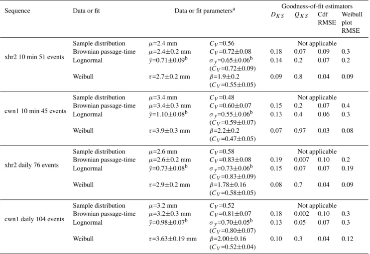
Fig. 2. Creep events (at a given point on a fault): the recurrent cumulative frequency-amplitude distributions for the sequences of 51 slip amplitudes of the xhr2 10 min record,(a)and(b), and of 45 slip amplitudes of the cwn1 10 min record,(c)and(d). In (a) and (c) the cumulative distribution functions of recurrent slip amplitudes are given as solid lines. The corresponding Weibull plots are given in (b) and (d) as diamonds. In all cases the data are compared with the best-fit Brownian passage-time distributions (dashdot lines), the best-fit lognormal distributions (short-dash lines), and the best-fit Weibull distributions (long-dash lines).

already contain only characteristic events. The telemetry res-olution acts here as the amplitude threshold 0.3 mm.

The frequency-amplitude distributions given in Fig. 1a– d clearly are not the power-law Gutenberg-Richter statis-tics normally associated with the frequency-magnitude dis-tribution of earthquakes in a large region (Gutenberg and Richter, 1954; Kanamori and Anderson, 1975; Pacheco et al., 1992; Rundle and Klein, 1993). This is not surprising since Gutenberg-Richter statistics are associated with earth-quakes that occur on many faults. For the recurrent statistics of “characteristic events” more repetitive distributions (with lower aperiodicity) should be considered.

The traditional way to construct the Gutenberg-Richter distribution is to integrate events from large to small am-plitudes. The cumulative distribution function (cdf) repre-sents the number of events with amplitudes equal or greater than the current and is not normalized. Gutenberg and Richter (1954) introduced this technique for the interoccur-rent statistics because the number of small events in a region is infinite and it is impossible to integrate cdf starting from zero. Frequency-size statistics in Fig. 1a–d have been con-structed in the similar way, only, in our case, for a

linear-linear scale for both axes. This technique is relevant and works well for the case of the interoccurrent statistics in a region. However, the recurrent frequency-size statistics have a tendency to be more periodic and the power law divergence of statistics at zero amplitude is absent in this case. There-fore, the using of the Gutenberg-Richter technique for the case of the recurrent statistics is confusing and not required. We will construct the recurrent statistics as it would be done by statisticians. For this purpose we integrate events

(7)

(a)

0 2 4 6 8 10

0.0 0.2 0.4 0.6 0.8 1.0

xhr2 daily event sequence Brownian passage-time fit Lognormal fit

Weibull fit

P

(

S

)

Slip amplitude S, mm _(b)

1 10

1E-3 0.01 0.1 1

1E-3 0.005 0.01 0.05 0.1 0.25 0.5 0.75 0.9 0.95 0.99 0.999

xhr2 daily event sequence Brownian passage-time fit Lognormal fit

Weibull fit

-ln(1-P

(

S

))

P

(

S

)

(c)

0 2 4 6 8 10

0.0 0.2 0.4 0.6 0.8 1.0

cwn1 daily event sequence Brownian passage-time fit Lognormal fit

Weibull fit

P

(

S

)

Slip amplitude S, mm _(d)

1 10

1E-3 0.01 0.1 1

1E-3 0.005 0.01 0.05 0.1 0.25 0.5 0.75 0.9 0.95 0.99 0.999

cwn1 daily event sequence Brownian passage-time fit Lognormal fit

Weibull fit

-ln(1-P

(

S

))

P

(

S

)

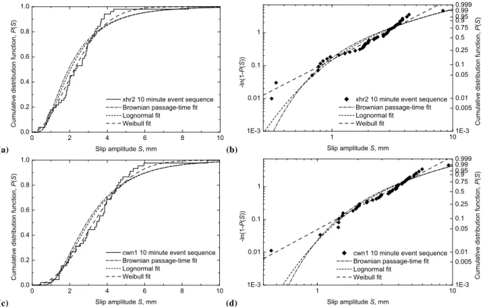
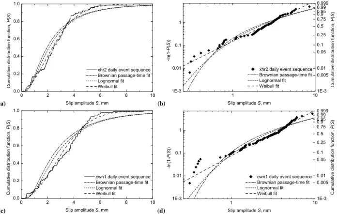
Fig. 3. Creep events (at a given point on a fault): the recurrent cumulative frequency-amplitude distributions for the sequences of 76 slip amplitudes of the xhr2 daily record,(a)and (b), and of 104 slip amplitudes of the cwn1 daily record, (c)and(d). In (a) and (c) the cumulative distribution functions of recurrent slip amplitudes are given as solid lines. The corresponding Weibull plots are given in (b) and (d) as diamonds. In all cases the data are compared with the best-fit Brownian passage-time distributions (dash-dot lines), the best-fit lognormal distributions (short-dash lines), and the best-fit Weibull distributions (long-dash lines).

In Fig. 2b and d the recurrent statistics for the xhr2 and cwn1 10 min event sequences are plotted in the form

−ln(1−P (S))versusSin log10–log10axes. In this form the Weibull distribution is a straight-line fit with slopeβso that this is known as a Weibull plot. Also included in these figures are the previous best-fits of the Brownian passage-time, log-normal, and Weibull distributions with RMSE in the log10– log10axes given in Table 1.

Equivalent results for 76 recurrent slip amplitudes for the xhr2 daily event sequence and 104 recurrent slip amplitudes for the cwn1 daily event sequence are given in Fig. 3a–d. The means, coefficients of variation, and parameters of fits are given in Table 1.

The goodness-of-fit estimators shown in Table 1 demon-strate that the fits of the Weibull distribution for all four sequences are better than those of either the lognormal or Brownian passage-time distributions. In particular, the val-ues ofDKSand RMSE for both the cdf and Weibull plots are significantly smaller, and the values ofQKSare significantly larger for the Weibull distribution than the corresponding val-ues for the fits of the other distributions. However, only the Brownian passage-time distribution for the daily records can

be rejected at the 5% confidence level. Also, direct visual in-spections indicate the strong tendency of the sample distribu-tions to be linear on Weibull plots, i.e., the intrinsic property of the Weibull distribution.

4 Slider-block model

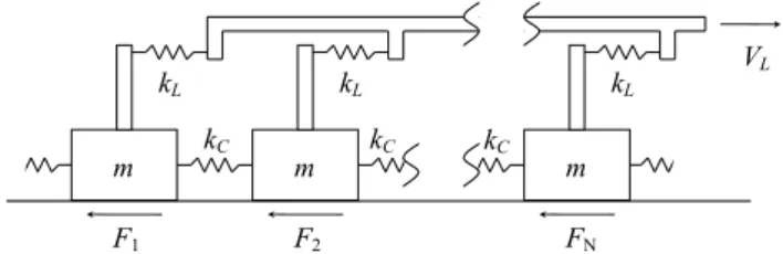
In this section we consider the behavior of a slider-block model in order to study the statistics of event sizes. We uti-lize the linear 500 block model considered by Abaimov et al. (2007b). The model is illustrated in Fig. 4. It is our ob-jective here to study the recurrent frequency-size statistics of the model with the same parameter values used in the recur-rent time-interval studies. Details of the model are given in Appendix C.

(8)

VL

kL

m m m

F₁ F₂ F_N

kC kC kC

Fig. 4.Illustration of one-dimensional slider-block model. A linear array ofN=500 blocks of mass m is pulled along a surface at a con-stant velocityV_Lby a loader plate. The loader plate is connected to each block with a loader spring with spring constantkLand

adja-cent blocks are connected by springs with spring constantkC. The

frictional resisting forces areF1,F2, ...,FN.

the infinite model; Abaimov, 2009). In the limit of infinite model size (infinite number of blocks) the frequency-size dis-tributions of events are power-laws. However for a model of finite size the statistics are influenced by the finite-size ef-fect. System-wide events occur instead of events with infi-nite size. The power-law distribution is still valid for smaller non-system wide events but the statistics of “virtual” events with sizes larger than the model size are accumulated in the statistics of system-wide events. The system-wide events can be associated with the characteristic events of a finite model. The term “characteristic” intrinsically assumes the presence of the finite size in the model because the infinite model at the critical state does not have a characteristic length. The same situation is observed in the case of earthquakes. The frequency-size statistics in a region are power-law distribu-tions. However, the characteristic events in this region are determined by the length of the largest fault (or fault seg-ment) and are in situ determined by the finite-size effect of the most catastrophic slip elongation that this region can sus-tain. Indeed, we do not expect the occurrence of events with magnitudes greater than e.g. 20 in any region of Earth in spite of the fact that the possibility of these events (events with ar-bitrarily large magnitudes) is always permitted by the power-law Gutenberg-Richter distribution without magnitude cut-offs. It is well accepted that Gutenberg-Richter distribution is not valid for datasets of strong earthquakes with magni-tudes greater than 8 (Kagan and Knopoff, 1976). Therefore, as it was first suggested by Abaimov et al. (2007b, 2008), we attribute the recurrent properties of characteristic events to the recurrent behavior of the model system-wide events.

First, we will consider the recurrent statistics at a given point on a fault. In the case of the slider-block model this cor-responds to a given block of the model. We consider statistics for the “strongest”, “weakest”, and “medium” blocks. As a strongest block we choose the block with the highest coeffi-cient of friction, i.e., a block with the highestβi. As a weak-est block we choose the block with the lowweak-est coefficient of friction. And as a medium block we choose the block with the friction coefficient which is close to the friction

coeffi-cient averaged over the model. As the size of an event we choose the total slip amplitude of the given block during this event.

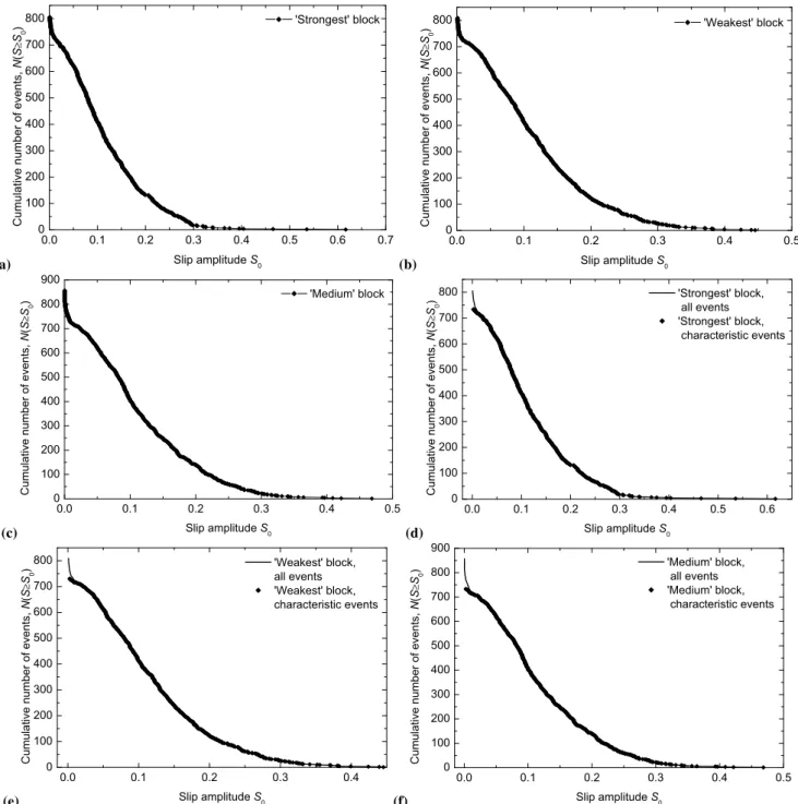
First we construct the cumulative recurrent statistics in the Gutenberg-Richter style. The frequency-amplitude distribu-tions of recurrent slip amplitudesP (S)for event sequences of the strongest, weakest and medium blocks are given as a function of block’s slip amplitudeSin Fig. 5a–c respectively. These figures are visually similar to Fig. 1a–d. We see here the same anomaly due to the presence of non-characteristic (non-system-wide) events. However, for these numerical simulations we have the opportunity to separate characteris-tic events directly as being system-wide events (without the introduction of the amplitude threshold). The cumulative re-current statistics of all events are compared to the statistics of only characteristic events in Fig. 5d–f. We see that indeed the influence of non-characteristic events results only in the distortion of the statistics at small amplitudes. As done in our study of the creep events (above), we will remove non-characteristic events from the statistics, integrate the cdf from small to large amplitudes, and normalize the statistics by di-viding by the total number of events.

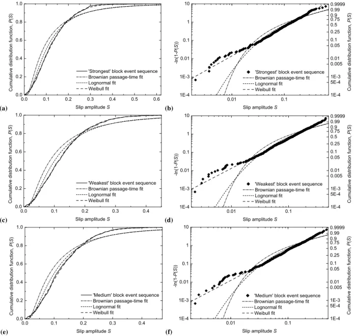
The cumulative distribution of recurrent slip amplitudes P (S)for the event sequences of the strongest, weakest, and medium blocks are given as functions of the slip amplitude Sin Fig. 6a, c, and e. The means and coefficients of varia-tion of these sequences are given in Table 2. Also included in Figs. 6a, c, and e are the best-fits (maximum likelihood) of the Brownian passage-time, lognormal, and Weibull distribu-tions. Both the parameters of these fits and the goodness-of-fit estimators are given in Table 2.

Figure 6b, d, and f present the Weibull plots corresponding to Fig. 6a, c, and e respectively. Also included in these Fig-ures are the corresponding best-fits of the Brownian passage-time, lognormal, and Weibull distributions with the RMSE in log10–log10axes given in Table 2.

Both the creep sequences and the sequences of the slider-block model investigated above are the sequencesat a given point on a fault. But for the slider-block model we can obtain sequenceson a given fault. We consider again the system-wide events as the characteristic events. Then we can con-sider energy dissipated by the whole model (by all blocks) during an event as the size of this event. Indeed, the energy dissipated by all blocks during an event is already not associ-ated with the slip amplitude at a given point of the model but is associated with the slip amplitude averaged over the model (roughly speaking, Eq. 1). The frequency-size statistics can be constructed both for energies and slip amplitudes. There-fore as the size of an event we can use the energy of this event as well as the slip amplitude. See below for a discussion of these differences.

(9)

(a)

0.0 0.1 0.2 0.3 0.4 0.5 0.6 0.7 0

100 200 300 400 500 600 700

800 'Strongest' block

N

(

S

≥

S0

)

Slip amplitude S

0 (b)

0.0 0.1 0.2 0.3 0.4 0.5

0 100 200 300 400 500 600 700

800 'Weakest' block

N

(

S

≥

S0

)

Slip amplitude S

0

(c)

0.0 0.1 0.2 0.3 0.4 0.5

0 100 200 300 400 500 600 700 800 900

'Medium' block

N

(

S

≥

S0

)

Slip amplitude S

0 (d)

0.0 0.1 0.2 0.3 0.4 0.5 0.6

0 100 200 300 400 500 600 700

800 'Strongest' block,

all events 'Strongest' block, characteristic events

N

(

S

≥

S0

)

Slip amplitude S

0

(e)

0.0 0.1 0.2 0.3 0.4

0 100 200 300 400 500 600 700

800 'Weakest' block,

all events 'Weakest' block, characteristic events

N

(

S

≥

S0

)

Slip amplitude S

0 (f)

0.0 0.1 0.2 0.3 0.4 0.5

0 100 200 300 400 500 600 700 800 900

'Medium' block, all events

'Medium' block, characteristic events

N

(

S

≥

S0

)

Slip amplitude S

0

Fig. 5. Slider-block model, recurrent events: cumulative number of events greater thanS0,N (S≥S0), versus slip amplitudeS0for event

sequences of the(a)strongest block,(b)weakest block, and(c)medium block (at a given point of the model). In(d),(e), and(f)the same statistics (solid lines) are compared to the statistics of only characteristic events. The cumulative distribution functions are integrated from large to small amplitudes and are not normalized (similar to the Gutenberg-Richter distribution except only linear scales for both axes).

in Table 3. Also included in Fig. 7a are the best-fits (maxi-mum likelihood) of the Brownian passage-time, lognormal, and Weibull distributions. Both the parameters of these fits and the goodness-of-fit estimators are given in Table 3.

Figure 7b presents the Weibull plot corresponding to Fig. 7a. Also included in this Figure are the correspond-ing best-fits of the Brownian passage-time, lognormal, and

Weibull distributions with the RMSE in log10–log10 axes given in Table 3.

(10)

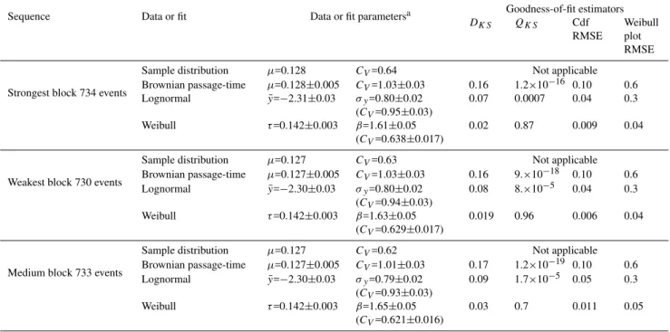
Table 2. Slider-block model: The recurrent slip amplitude statistics at a given point of the model. For all sequences the parameters of the best-fit Brownian passage-time, lognormal, and Weibull distributions are given as well as the goodness-of-fit estimators. Units of slip amplitude are non-dimensional, introduced by Eq. (C5).

DKS QKS Cdf RMSE

Weibull plot RMSE

Strongest block 734 events

Sample distribution µ=0.128 CV=0.64 Not applicable

Brownian passage-time µ=0.128±0.005 CV=1.03±0.03 0.16 1.2×10−16 0.10 0.6

Lognormal y¯=−2.31±0.03 σy=0.80±0.02

(CV=0.95±0.03)

0.07 0.0007 0.04 0.3

Weibull τ=0.142±0.003 β=1.61±0.05

(CV=0.638±0.017)

0.02 0.87 0.009 0.04

Weakest block 730 events

Brownian passage-time µ=0.127±0.005 CV=1.03±0.03 0.16 9.×10−18 0.10 0.6

Lognormal y¯=−2.30±0.03 σy=0.80±0.02

(CV=0.94±0.03)

0.08 8.×10−5 0.04 0.3

Weibull τ=0.142±0.003 β=1.63±0.05

(CV=0.629±0.017)

0.019 0.96 0.006 0.04

Medium block 733 events

Brownian passage-time µ=0.127±0.005 CV=1.01±0.03 0.17 1.2×10−19 0.10 0.6

Lognormal y¯=−2.30±0.03 σy=0.79±0.02

(CV=0.93±0.03)

0.09 1.7×10−5 0.05 0.3

Weibull τ=0.142±0.003 β=1.65±0.05

(CV=0.621±0.016)

0.03 0.7 0.011 0.05

a_{The error bars are 95% confidence limits.}

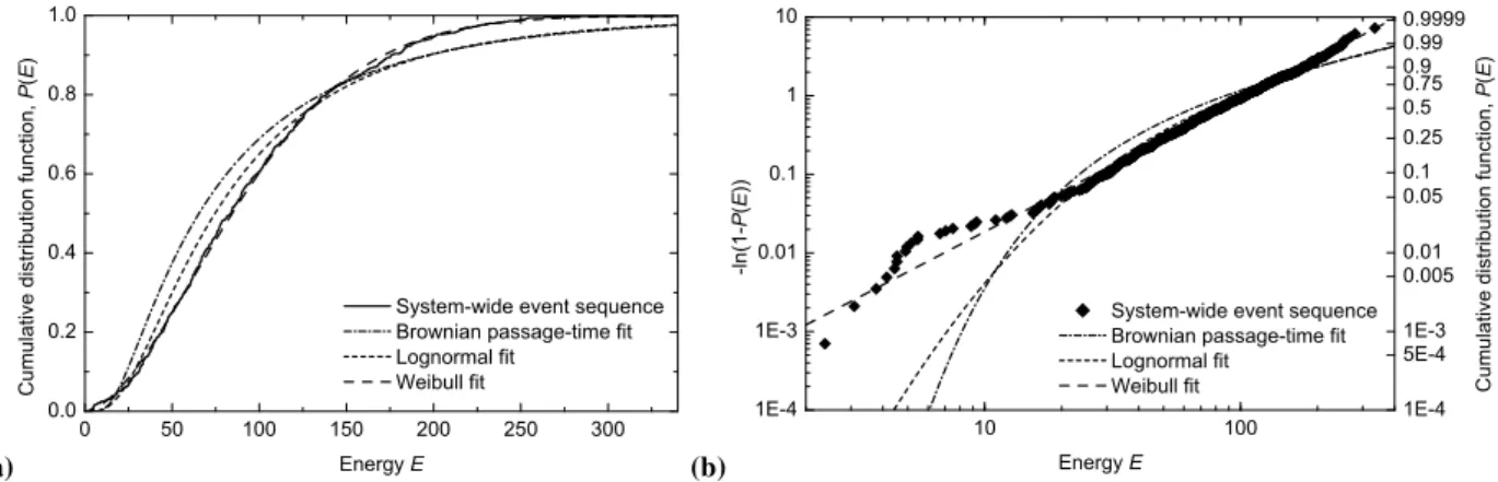
Table 3.Slider-block model: The cumulative distribution of recurrent energies for the system-wide event sequence (on a given fault). The parameters of the best-fit Brownian passage-time, lognormal, and Weibull distributions are given as well as the goodness-of-fit estimators. Units of energy are non-dimensional, introduced by Eq. (C5).

DKS QKS Cdf RMSE

Weibull plot RMSE

Energies dissipated Sample distribution µ=94. CV=0.61 Not applicable

during 715 system- Brownian passage-time µ=94.±3. CV=0.95±0.03 0.14 1.4×10−13 0.09 0.5

wide events Lognormal y¯=4.31±0.03 σy=0.76±0.02 (CV=0.88±0.03) 0.07 0.0009 0.04 0.3

Weibull τ=105.±2. β=1.70±0.05 (CV=0.607±0.016) 0.02 0.88 0.009 0.05

significantly smaller, and the values ofQKSare significantly larger for the Weibull distribution than the corresponding val-ues for the fits of other distributions. Also, direct visual in-spections indicate the strong tendency of the sample distribu-tions to be linear on the Weibull plots, a recognized property of the Weibull distribution.

The frequency-size statistics can be constructed both for energies and slip amplitudes. However, the fact that both statistics have the same behavior (linear on Weibull plot) means that the applied distribution should be invariant rel-atively a power law transformation. Indeed, the energy dis-sipated by all blocks during an event is associated with the

(11)

(a)

0.0 0.1 0.2 0.3 0.4 0.5 0.6

0.0 0.2 0.4 0.6 0.8 1.0

'Strongest' block event sequence Brownian passage-time fit Lognormal fit

Weibull fit

P

(

S

)

Slip amplitude S _(b)

0.01 0.1 1E-4 1E-3 0.01 0.1 1 10 1E-4 5E-4 1E-3 0.005 0.01 0.05 0.1 0.25 0.5 0.75 0.9 0.99 0.9999

'Strongest' block event sequence Brownian passage-time fit Lognormal fit Weibull fit -ln(1-P ( S ))

Slip amplitude S

P

(

S

)

(c)

0.0 0.1 0.2 0.3 0.4

0.0 0.2 0.4 0.6 0.8 1.0

'Weakest' block event sequence Brownian passage-time fit Lognormal fit

Weibull fit

P

(

S

)

Slip amplitude S _(d)

0.01 0.1 1E-4 1E-3 0.01 0.1 1 10 1E-4 5E-4 1E-3 0.005 0.01 0.05 0.1 0.25 0.5 0.75 0.9 0.99 0.9999

'Weakest' block event sequence Brownian passage-time fit Lognormal fit Weibull fit -ln(1-P ( S ))

Slip amplitude S

P

(

S

)

(e)

0.0 0.1 0.2 0.3 0.4

0.0 0.2 0.4 0.6 0.8 1.0

'Medium' block event sequence Brownian passage-time fit Lognormal fit

Weibull fit

P

(

S

)

Slip amplitude S _(f)

0.01 0.1 1E-4 1E-3 0.01 0.1 1 10 1E-4 5E-4 1E-3 0.005 0.01 0.05 0.1 0.25 0.5 0.75 0.9 0.99 0.9999

'Medium' block event sequence Brownian passage-time fit Lognormal fit Weibull fit -ln(1-P ( S ))

Slip amplitude S

P

(

S

)

Fig. 6. Slider-block model: The recurrent cumulative frequency-amplitude distributions for the sequences of 734 slip amplitudes of the strongest block,(a)and(b), of 730 slip amplitudes of the weakest block,(c)and(d), and of 733 slip amplitudes of the medium block (at a given point of the model). In(a),(c), and(e)the cumulative distribution functions of recurrent slip amplitudes are given as solid lines. The corresponding Weibull plots are given in(b),(d), and(f)as diamonds. In all cases the data are compared with the best-fit Brownian passage-time distributions (dash-dot lines), the best-fit lognormal distributions (short-dash lines), and the best-fit Weibull distributions (long-dash lines).

an additional verification that the Weibull distribution is the relevant distribution.

Thus, the Weibull distribution is the preferred distribution of three trials both for the creep event sequences and for the sequences of characteristic events in the slider-block model analyzed here. It is encouraging that independent analyses of signals which are considered good proxies for earthquake behavior, one natural and one simulated, produce consistent results.

(12)

(a)

0 50 100 150 200 250 300

0.0 0.2 0.4 0.6 0.8 1.0

System-wide event sequence Brownian passage-time fit Lognormal fit

Weibull fit

P

(

E

)

Energy E (b)

10 100

1E-4 1E-3 0.01 0.1 1 10

1E-4 5E-4 1E-3 0.005 0.01 0.05 0.1 0.25 0.5 0.75 0.9 0.99 0.9999

System-wide event sequence Brownian passage-time fit Lognormal fit

Weibull fit

-ln(1-P

(

E

))

Energy E

P

(

E

)

Fig. 7.Slider-block model: The recurrent cumulative frequency-energy distribution for the sequence of 715 system-wide events (on a given fault). In(a)the cumulative distribution function of recurrent energies is given as a solid line. The corresponding Weibull plot is given in(b) as diamonds. In both cases the data are compared with the best-fit Brownian passage-time distribution (dash-dot lines), the best-fit lognormal distribution (short-dash lines), and the best-fit Weibull distribution (long-dash lines).

The similarity of Weibull exponents of the creep events and slider-block model is valid and for the recurrent time-interval statistics as well. The recurrent time-interval be-havior of the characteristic creep events was investigated by Abaimov et al. (2007a). The Weibull distribution was found to be the preferred distribution for the recurrent time-interval statistics and the exponents β of the best-fit Weibull dis-tributions produced values ranging from 2.2 to 2.7. This corresponds to an aperiodicity of the applied distribution of CV=0.40−0.48. In parallel, the recurrent time-interval be-havior of the system-wide events of the stiff slider-block model was investigated by Abaimov et al. (2007b). The Weibull distribution also was found to be the preferred dis-tribution for the recurrent time-interval statistics and the ex-ponentβ of the trial Weibull distribution equaled 2.6. This corresponds to an aperiodicity of the applied distribution of CV=0.41, which falls within the range of the creep events results,CV=0.40−0.48. Therefore, both these independent systems whose applicability to earthquakes has been fre-quently noted and studied (Abaimov et al., 2007a; Abaimov et al., 2007b; Carlson and Langer, 1989), creep events and the slider-block model, exhibit closely related recurrent be-havior of both frequency-size and time-interval statistics. This supports our hypothesis that the stiff slider-block model, which obeys the principles of critical point (Abaimov, 2009), could represent the behavior of actual sequences of charac-teristic earthquakes on a given fault.

5 Sand-pile model

The stiff slider-block model obeys the principles of self-organized criticality (Abaimov et al., 2007b; Carlson and Langer, 1989). Applicability of this concept to earthquakes is discussed in the literature (Bak et al., 2002). Therefore it would be interesting to take a look at the recurrent

frequency-size behavior of a sand-pile model as a classical representa-tive of this theory (Bak et al., 1988). We utilize the simplest variation of two-dimensional sand-pile model. A square grid of 100 by 100 sites is strewn with sand grains. When a site accumulates four or more grains it becomes unstable and re-distributes four grains to its four neighbors. Instability of one site can trigger instability of others, forming a complex avalanche in the system. The sand redistribution during an avalanche is assumed to be much faster than the rate of the stable sand accumulation (similarly, velocity of earthquake propagation is much faster than tectonic rate of stress accu-mulation). Therefore, the slow sand strewing is neglected during avalanches. Boundaries of the model are assumed to be free so the sand can leave the model at boundaries when it is redistributed by a boundary site.

To construct the recurrent statistics at a given point of the model we choose a site in the middle of the lattice. All avalanches with participation at this site will be counted as events at this site of the model. To separate characteristic events we need to construct a criterion similar to the system-wide criterion for the slider-block. For the sand-pile model we choose a percolation criterion as a criterion for an event to be characteristic: An event will be considered as charac-teristic if it percolates the lattice and connects all four bound-aries (up-right-down-left percolation). As the size of an event we choose the number of different sites participating in this avalanche. Each site can repeatedly lose stability during this event but will be counted only once in the size of the event.

(13)

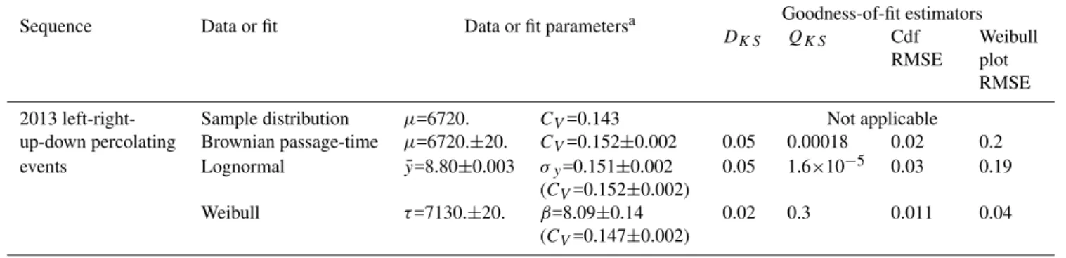
Table 4.Sand-pile model: The cumulative recurrent frequency-size distribution for the sequence of percolating events (at a given point of the model). The parameters of the best-fit Brownian passage-time, lognormal, and Weibull distributions are given as well as the goodness-of-fit estimators.

DKS QKS Cdf

RMSE

Weibull plot RMSE

2013 left-right- Sample distribution µ=6720. CV=0.143 Not applicable

up-down percolating Brownian passage-time µ=6720.±20. CV=0.152±0.002 0.05 0.00018 0.02 0.2

events Lognormal y=8.80_¯ _±0.003 σy=0.151±0.002

(CV=0.152±0.002)

0.05 1.6_×10−5 0.03 0.19

Weibull τ=7130._±20. β=8.09_±0.14

(CV=0.147±0.002)

0.02 0.3 0.011 0.04

(a)

2000 4000 6000 8000 10000

0.0 0.2 0.4 0.6 0.8 1.0

Sequence of percolating events Brownian passage-time fit Lognormal fit

Weibull fit

P

(

S

)

Event size S _(b)

4000 6000 8000 10000

1E-5 1E-4 1E-3 0.01 0.1 1 10

1E-5 1E-4 5E-4 1E-3 0.005 0.01 0.05 0.1 0.25 0.5 0.75 0.9 0.99 0.9999

Sequence of percolating events Brownian passage-time fit Lognormal fit

Weibull fit

-ln(1-P

(

S

))

Event size S

P

(

S

)

Fig. 8.Sand-pile model: The recurrent cumulative frequency-size distribution for the sequence of 2013 percolating events (at a given point of the model). In(a)the cumulative distribution function of recurrent event sizes is given as a solid line. The corresponding Weibull plot is given in(b)as diamonds. In both cases the data are compared with the best-fit Brownian passage-time distribution (dash-dot lines), the best-fit lognormal distribution (short-dash lines), and the best-fit Weibull distribution (long-dash lines).

Figure 8b presents the Weibull plot corresponding to Fig. 8a. Also included in this figure are the correspond-ing best-fits of the Brownian passage-time, lognormal, and Weibull distributions with the RMSE in log10–log10 axes given in Table 4.

Again, the Weibull distribution is the best-fit distribution. However, now its exponentβhas much higher valueβ=8.09 which corresponds to the aperiodicity CV=0.15. This is likely due to the effect of the percolation criterion as a cri-terion for an event to be characteristic. Although for this case we see the same functional (Weibull) dependence of the recurrent frequency-size statistics, the sand-pile model has another symmetry and belongs to another universality class with different anomalous dimensions. This question requires further investigation.

6 Conclusions

Recurrent frequency-size distributions play an important role in earthquake hazard assessments. However, observed se-quences of characteristic earthquakes at a given point on a fault or on a given fault are not able to differentiate among alternative statistical distributions. To overcome this diffi-culty this paper investigates the sequences of creep events on the creeping section of the San Andreas fault. For four se-quences the Weibull distribution is shown to be the preferred distribution. Applicability of this distribution is confirmed by the goodness-of-fit estimators. Direct visual inspections also support the applicability of the Weibull distribution be-cause the sample distribution has the tendency to be linear on the Weibull plot.

(14)

applicability of the Weibull distributions to the recurrent frequency-size statistics.

Another noteworthy fact is that both the creep event se-quences and the sese-quences of system-wide events of the slider-block model have similar values of coefficients of vari-ationCV=0.47÷0.64 for the recurrent frequency-size statis-tics. The same tendency was also found by Abaimov et al. (2007a,b) for the recurrent time-interval behavior of these two systems. The fact that two independent systems whose applicability to earthquakes is often discussed in the litera-ture have closely related recurrent behavior supports the hy-pothesis that these two systems actually represent the recur-rent earthquake behavior on a given fault or fault segment.

The recurrent statistics at a given point on a fault or on a given fault can contain both characteristic and non-characteristic events. For the frequency-size statistics Figs. 1 and 5 suggest that the non-characteristic events are described by a distribution which is different from the distribution of characteristic events. Indeed, for the mutual statistics of both characteristic and non-characteristic events in Figs. 1 and 5 we see the anomaly for small size events which clearly indi-cates the mixture of two different statistics. The same ten-dency is seen for the time-interval statistics. Of primary in-terest is the distribution of events with large sizes. Therefore it is reasonable to filter off the non-characteristic events and to study only the pure statistics of characteristic events as has been done in this paper.

However when we study the recurrent statistics of charac-teristic events the word “characcharac-teristic” assumes that there is a characteristic length in the system. This length rep-resents the length of the fault or fault segment or, in other words, the size of the system. Therefore the recurrent statis-tics of characteristic events are actually the result of the fi-nite size effect in the system when we consider only events whose correlation length exceeds the system size (system-wide events). Both time-interval and frequency-size recur-rent statistics are determined by the finite size effect there-fore it is peculiar that in the case of the ‘earthquake similar systems’ such as the stiff slider-block model or creep events this finite size effect has a similar appearance (the Weibull distribution) both for the time-interval and frequency-size statistics. An even more important fact is that not only both the recurrent time-interval and frequency-size statistics of characteristic events obey the Weibull distribution but also that the exponents of these distributions have similar values. This provides coefficients of variation of 0.40–0.48 for the recurrent time-intervals of creep events, 0.47–0.58 for the recurrent sizes of creep events, 0.41 for the recurrent time-intervals in the slider-block model, and 0.61–0.64 for the re-current sizes in the slider block model. We see that the co-efficients of variation have similar values both for the time-interval and frequency-size statistics (only for the recurrent sizes of the characteristic events in the slider-block model we have slightly higher but still close values). This supports the point of view that the finite-size effect, which determines

the behavior of characteristic events in the model, prescribes not only the same shape (Weibull) but also the same coeffi-cient of variation (in the range 0.40–0.64) both for the recur-rent time-interval and frequency-size statistics. The validity of this hypothesis would provide a unique opportunity to re-store the recurrent frequency-size statistics of characteristic earthquakes if we know their recurrent time-interval behavior from paleo-studies.

An interesting question is whether the statistical variabil-ity of slip magnitudes can be obtained for actual earthquakes. Unfortunately a coefficient of variation of 0.5 implies only a 0.1 magnitude variability for a magnitude six earthquake. This is outside the accuracy of magnitude specification. Thus our studies of creep events provide a unique opportunity to better understand the relationship between recurrent time-interval and frequency-size statistics.

The strong similarities between the recurrent time-interval and frequency-size statistics are evidence for their comple-mentarity. This complementarity supports the applicability of either time-predictable or slip-predictable forecast mod-els, however we have shown that these forecast models are not applicable to the recurrent statistics of the creep events (Abaimov et al., 2007a). Nevertheless, the applicability of Weibull statistics with similar coefficients of variation is striking. The general concept of complementarity appears to be valid but noise prevents predictability.

Appendix A

Applicable distributions

Three widely used statistical distributions in geophysics are the Brownian passage-time, lognormal, and Weibull. We compare each of them with our data (sample distribution). A1 Brownian passage-time distribution

The probability density function (pdf) of amplitudesS for the Brownian passage-time distribution is given by (Chhikara and Folks, 1989)

p(S)₌ µ 2π C_V2S3

!1₂

exp

"

−(S−µ)

2

2C2_VµS

#

(A1)

(15)

A2 Lognormal distribution

The lognormal is one of the most widely used statistical dis-tributions in a wide variety of fields. The pdf of amplitudesS for the lognormal distribution is given by (Patel et al., 1976)

p(S)₌ 1 (2π )1/2_σ

yS exp

"

−(lnS− ¯y)

2

2σ2 y

#

(A2)

The lognormal distribution can be transformed into the normal distribution by making the substitution y₌lnS; y_¯ andσy are the mean and standard deviation of this equiva-lent normal distribution. The meanµ, standard deviationσ, and aperiodicity (coefficient of variation)CV for the lognor-mal distribution are given by

µ₌exp

"

¯

y₊σ 2 y 2

#

, σ ₌µ

q

eσy2₋_1,_and

CV = σ µ =

q

eσy2 ₋₁ _(A3)

The corresponding cdfP (S)for the lognormal distribution is

P (S)₌1

2 1+erf

"

lnS_{− ¯}y

√

2σy

#!

(A4)

whereerf (x)₌√2

π x

R

0

e−y2dy is the error function. The log-normal distribution is closely related to the log-normal distribu-tion and is often used when an a priori positive quantity is distributed normally.

A3 Weibull distribution

The pdf for the Weibull distribution is given by (Patel et al., 1976)

p(S)₌β τ

_S

τ

β−1

exp

"

− _S

τ

β#

(A5)

whereβ andτ are fitting parameters. The meanµand the aperiodicity (coefficient of variation)CV of the Weibull dis-tribution are given by

µ₌τ Ŵ

1+ 1

β

(A6)

CV =



 

 

Ŵ1₊_β2

h

Ŵ1+β1

i2−1 

 

 

1 2

(A7)

whereŴ(x) is the gamma function of x. The cdf for the Weibull distribution is given by

P (S)₌1−exp

"

− _S

τ

β#

(A8)

Ifβ=1 the Weibull distribution becomes the exponential distribution with σ=µ and CV=1. In the limit β→+∞ the Weibull distribution becomes exactly repetitive (a δ-function) with σ₌CV=0. The Weibull distribution is often used in engineering because in accordance with the weak-link hypothesis this distribution represents the strength of materials (Meeker and Escobar, 1991; Weibull, 1951).

Appendix B

Measures of goodness-of-fit

In order to determine whether a specific distribution is an applicable representation of our statistics, it is necessary to utilize measures of goodness-of-fit. Many such tests are available (Press et al., 1995). In this paper we quantify the goodness-of-fit of distributions using three tests.

B1 One-sample Kolmogorov-Smirnov test

The first measure we employ is the one-sample Kolmogorov-Smirnov test (Press et al., 1995). To use this test the maxi-mum absolute differenceDKSbetween the cdf of the sample distribution (actual data)yi and the fitted distribution

⌢

y_i is determined:

DKS=max

yi−

⌢

y_i

(B1)

Then the significance level probability of the goodness-of-fit (the probability that the trial distribution is relevant) is given by

QKS(λ)=2

+∞ X

i=1

(₋1)i−1e−2i2λ2 (B2)

where λ₌DKS

√

n₊0.12₊0.11_√ n

, (B3)

andnis the number of data points. The preferred distribution has the smallest value ofDKSand the largest value ofQKS. B2 Root mean squared error test

(16)

divided by the difference between the number of data points and the number of fitting parameters

RMSE= v u u u t

n

P

i=1 (yi −

⌢

y_i)2

n₋k (B4)

whereyi are the sample distribution (actual data),

⌢

y_iare pre-dicted fit values,nis the number of data point, andkis the number of fitting parameters (k=2 for our three distributions). This test is also known as the fit standard error and the stan-dard error of the regression. The preferred distribution has the smallest RMSE value.

It should be noted that the data points in the cumulative distribution function or its specific plot are dependent and, therefore, the RMSE measure is not applicable rigorously to estimate the deviation of the distribution. However, we still apply this measure because it serves as a good indicator of the local pdf deviations. A local deviation of pdf between the sample and trial distributions causes the constant shift of one distribution relative to another on the cdf plot and, correspondently, high values of the RMSE measure. B3 Visual inspection

In spite of its simplicity a visual inspection often plays an important role in verifying the applicability of a statistical distribution. For this purpose, a specific plot usually is used where the trial distribution becomes a straight line. For ex-ample, if the trial distribution is the Weibull distribution the specific plot (called in this case the “Weibull” plot) is con-structed in the form−ln(1−P (S)) versusS in log10–log10 axes. In this form the Weibull distribution is a straight line with slopeβ. The difference between sample and trial dis-tributions, which is usually disguised on a usual cdf plot, is magnified and clearly exposed on a specific plot of the trial distribution. Therefore the visual inspection of a sample dis-tribution (to determine whether or not it is a straight line on a specific plot) serves as an important goodness-of-fit esti-mator. Because the result of this paper is the preference of the Weibull distribution, all results will be demonstrated on “Weibull” plots as well as cdf plots.

Appendix C

Formulation of the slider-block model

The slider-block model utilized in this paper is a varia-tion of the linear slider-block model which Carlson and Langer (1989) used to illustrate the self-organization of such models. We consider a linear chain of 500 slider blocks of massmpulled over a surface at a constant velocityVLby a loader plate as illustrated in Fig. 4. Each block is connected to the loader plate by a spring with spring constantkL. Ad-jacent blocks are connected to each other by springs with

spring constantkC. Boundary conditions are assumed to be periodic: the last block is connected to the first one.

The blocks interact with the surface through friction. In this paper we prescribe a static-dynamic friction law. The static stability of each slider-block is given by

kLyi+kC(2yi −yi−1−yi+1) < FSi (C1) whereFSi is the maximum static friction force on blocki holding it motionless, andyiis the position of blockirelative to the loader plate.

During strain accumulation due to loader plate motion, all blocks are motionless relative to the surface and have the same increase in their coordinates relative to the loader plate

dyi

dt =VL (C2)

When the cumulative force of the springs connecting to block iexceeds the maximum static frictionFSi, the block begins to slide. We include inertia, and the dynamic slip of blocki is controlled by the equation

md 2_y

i

dt2 +kLyi+kC(2yi −yi−1−yi+1)=FDi (C3) whereFDi is the dynamic (sliding) frictional force on block i. The loader plate velocity is assumed to be much smaller than the slip velocity, requiring

VL≪ F_Sref

√

kLm

(C4) so the movement of the loader plate is neglected during a slip event (F_Sref is the minimum value of all FSi). The sliding of one block can trigger the instability of the other blocks forming a many block event. When the velocity of a block is zero it sticks with zero velocity.

It is convenient to introduce the non-dimensional variables and parameters

τf =t

r

kL m, τs =

t kLVL F_Sref , Yi =

kLyi F_Sref

, φ₌ FSi FDi ,

α₌ kC kL

, βi = FSi

F_Sref (C5)

The ratio of static to dynamic frictionφis assumed to be the same for all blocks but the values themselvesβi vary from block to block withF_Sref as a reference value of the static frictional force. Stress accumulation occurs during the slow timeτs when all blocks are stable, and slip of blocks occurs during the fast timeτf when the loader plate is assumed to be approximately motionless.

In terms of these non-dimensional variables the static sta-bility condition Eq. (C1) becomes

(17)

the strain accumulation Eq. (C2) becomes dYi

dτS =

1 (C7)

and the dynamic slip Eq. (C3) becomes d2Yi

dτ_f2 +Yi+α (2Yi −Yi−1−Yi+1)= βi

φ (C8)

Before obtaining solutions, it is necessary to prescribe the parametersφ,α, andβi. The parameterαis a tuning param-eter and is the stiffness of the system. For theαparameter, as the stiffness of the model, we should use some high value. In-deed, the stiffness of the fault may be lower than the stiffness of the surrounding intact rocks but we should associate the springs to the loader here with the stiffness of the total elon-gation of a tectonic plate. Therefore the fault must be much stiffer than the loader elements. We considerα=1000 which corresponds to a very stiff model. The important fact here is that we use this high value for the stiffness because the stiff slider-block model is believed to represent the proper-ties of earthquake recurrence (Abaimov et al., 2007b, 2008). When the stiffness of the system tends to infinity, the model reaches its critical point (Abaimov, 2009). At the state close to the critical the system exhibits power-law behavior.

The ratioφof static friction to dynamic friction is taken to be the same for all blocksφ₌1.5, while the values of fric-tional parametersβi are assigned to blocks by uniform ran-dom distribution from the range 1<βi<3.5. This random variability in the system is a “noise” required to thermalize the system and generate event variability.

The loader plate springs of all blocks extend according to Eq. (C7) until a block becomes unstable from Eq. (C6). The dynamic slip of that block is calculated using the Runge-Kutta numerical method to obtain a solution of Eq. (C8). A coupled 4th-order iterational scheme is used, and all equa-tions are solved simultaneously (the Runge-Kutta coeffi-cients of neighboring blocks participate in the generation of the next order Runge-Kutta coefficient for the given block). The dynamic slip of one block may trigger the slip of other blocks and the slip of blocks is followed until they all become stable. Then the procedure repeats.

Acknowledgements. The work of SGA and KT was funded by

the NSERC and Benfield/ICLR Industrial Research Chair in Earthquake Hazard Assessment. The authors would like to thank for fruitful comments Euan Smith and unknown Referee.

Edited by: G. Zoeller

Reviewed by: E. Smith and another anonymous Referee

References

Abaimov, S. G., Turcotte, D. L., and Rundle, J. B.: Recurrence-time and frequency-slip statistics of slip events on the creeping section of the San Andreas fault in central California, Geophys. J. Int., 170, 1289–1299, 2007a.

Abaimov, S. G., Turcotte, D. L., Shcherbakov, R., and Rundle, J. B.: Recurrence and interoccurrence behavior of self-organized complex phenomena, Nonlin. Processes Geophys., 14, 455–464, 2007b,

http://www.nonlin-processes-geophys.net/14/455/2007/. Abaimov, S. G., Turcotte, D. L., Shcherbakov, R., Rundle, J. B.,

Yakovlev, G., Goltz, C., and Newman, W. I.: Earthquakes: Re-currence and interocRe-currence times, Pure Appl. Geophys., 165, 777–795, 2008.

Abaimov, S. G.: Critical behavior of slider-block model, arXiv:0902.3767, 2009.

Bak, P., Tang, C., and Wiesenfeld, K.: Self-organized criticality, Phys. Rev. A., 38, 364–374, 1988.

Bak, P., Christensen, K., Danon, L., and Scanlon, T.: Uni-fied scaling law for earthquakes, Phys. Rev. Lett., 88, 178501, doi:10.1103/PhysRevLett.88178501, 2002.

Bakun, W. H., Aagaard, B., and Dost, B., et al.: Implications for prediction and hazard assessment from the 2004 Parkfield earth-quake, Nature, 437, 969–974, 2005.

Biasi, G. P., Welden, R. J., Fumal, T. E., and Seitz, G. G.: Pa-leoseismic event dating and the conditional probability of large earthquakes on the southern San Andreas fault, California, Bull. Seism. Soc. Am., 92, 2761–2781, 2005.

Carlson, J. M. and Langer, J. S.: Mechanical model of an earthquake fault, Phys. Rev. A, 40, 6470–6484, 1989.

Chhikara, R. S. and Folks, J. L.: The Inverse Gaussian Distribution: Theory, Methodology, and Applications, Marcel Dekker, New York, 1989.

Gutenberg, B. and Richter, C. F.: Seismicity of the Earth and Asso-ciated Phenomenon, Princeton University Press, Princeton, 2nd ed., 1954.

Kagan, Y. and Knopoff, L.: Statistical search for nonrandom fea-tures of seismicity of strong earthquakes, Phys. Earth Planet. In-ter., 12, 291–318, 1976.

Kanamori, H. and Anderson, D. L.: Theoretical basis of some em-pirical relations in seismology, Bull. Seism. Soc. Am., 65, 1073– 1095, 1975.

Langbein, J.: Download fault creep data from central Cal-ifornia, http://quake.usgs.gov/research/deformation/monitoring/ downloadcreep.html, 2006.

Matthews, M. V., Ellsworth, W. L., and Reasenberg, P. A.: A Brow-nian model for recurrent earthquakes, Bull. Seism. Soc. Am., 92, 2233–2250, 2002.

Meeker, W. Q. and Escobar, L. A.: Statistical Methods for Reliabil-ity Data, John Wiley, New York, 1991.

Molchan, G. M.: Strategies in strong earthquake prediction, Phys. Earth. Planet. Int., 61, 84–98, 1990.

Molchan, G. M.: Structure of optimal strategies in earthquake pre-diction, Tectonophys., 193, 267–276, 1991.

Nishenko, S. P. and Buland, R.: A generic recurrence interval dis-tribution for earthquake forecasting, Bull. Seism. Soc. Am., 77, 1382–1399, 1987.