Permafrost temperature and active-layer thickness of Yakutia with 0.5 degree spatial resolution for model evaluation

(1)

ESSDD

6, 153–162, 2013

Permafrost state maps of Yakutia

C. Beer et al.

Title Page

Abstract Instruments

Data Provenance & Structure

Tables Figures

◭ ◮

Back Close

Full Screen / Esc

Printer-friendly Version Interactive Discussion

Discussion

P

a

per

|

Dis

cussion

P

a

per

|

Discussion

P

a

per

|

Discussio

n

P

a

per

Earth Syst. Sci. Data Discuss., 6, 153–162, 2013 www.earth-syst-sci-data-discuss.net/6/153/2013/ doi:10.5194/essdd-6-153-2013

Open

Access

Earth System

Science

Data

D

iscussions

This discussion paper is/has been under review for the journal Earth System Science Data (ESSD). Please refer to the corresponding final paper in ESSD if available.

Permafrost temperature and active-layer

thickness of Yakutia with 0.5 degree

spatial resolution for model evaluation

C. Beer1,2, A. N. Fedorov3,4, and Y. Torgovkin3

1

Max Planck Institute for Biogeochemistry, Jena, Germany 2

Department of Applied Environmental Science (ITM) and the Bert Bolin Centre for Climate Research, Stockholm University, Stockholm, Sweden

3

Melnikov Permafrost Institute SB RAS, Yakutsk, Russia 4

International Center BEST, North-Eastern Federal University, Yakutsk, Russia

Received: 20 February 2013 – Accepted: 6 May 2013 – Published: 27 May 2013

Correspondence to: C. Beer ([email protected])

(2)

ESSDD

6, 153–162, 2013

C. Beer et al.

Title Page

Tables Figures

◭ ◮

Back Close

Full Screen / Esc

Discussion

P

a

per

|

Dis

cussion

P

a

per

|

Discussion

P

a

per

|

Discussio

n

P

a

per

|

Abstract

Based on the map of landscapes and permafrost conditions in Yakutia (Merzlotno-landshaftnaya karta Yakutskoi0 ASSR, Gosgeodeziya SSSR, 1991), rasterized maps of permafrost temperature and active-layer thickness of Yakutia, East Siberia were derived. The mean and standard deviation at 0.5 degree grid cell size are es-5

timated by assigning a probability density function at 0.001 degree spatial res-olution. The gridded datasets can be accessed at the PANGAEA repository (doi:10.1594/PANGAEA.808240). Spatial pattern of both variables are dominated by a climatic gradient from north to south, and by mountains and the soil type distribu-tion. Uncertainties are highest in mountains and in the isolated permafrost zone in the 10

south. The maps are best suited as a benchmark for land surface models which include a permafrost module.

1 Introduction

Physical and biogeochemical processes in permafrost underlain landscapes in high latitudes are important components of the Earth system. This importance has let to re-15

cent advancements of heat conduction and phase change representations in land sur-face schemes of Earth system models (e.g. Lawrence and Slater, 2005; Koven et al., 2009). These models calculate the physical and biogeochemical state of the ecosys-tem for large grid cells (approximate 0.5 to 3.75 degree spatial resolution) by using soil texture and land cover information as well as climate data from the atmospheric 20

(3)

ESSDD

6, 153–162, 2013

C. Beer et al.

Title Page

Tables Figures

◭ ◮

Back Close

Full Screen / Esc

Discussion

P

a

per

|

Dis

cussion

P

a

per

|

Discussion

P

a

per

|

Discussio

n

P

a

per

change including the effects of thawing permafrost on vegetation functions and carbon dioxide and methane production from carbon-rich permafrost soils.

In global models, big assumptions are made about initialization of state variables, such as soil temperature, and about parameter values, such as snow thermal param-eters. Therefore, the validation of the simulation of recent permafrost state variables, 5

such as permafrost temperature or active-layer thickness is an important step before projecting future conditions. For doing so, comparisons to databases of point measure-ments, such as GTN-P (Romanovsky et al., 2010) or CALM (Brown et al., 2000) are powerful tools (e.g. Oelke et al., 2003; Beer et al., 2007; Lawrence et al., 2008). How-ever, for such point-wise comparisons the models should be run using site-level soil 10

texture type information and site-level meteorological observations, which is an enor-mous effort for a large set of sites, such as represented by CALM. In addition, the com-parison of a large-scale temperature value representing a mean for an 0.5 degree grid cell with a single measurement inside that grid cell is highly unreliable since local con-ditions and processes, such as the horizonthal water flow are usually not represented 15

by a site-level run of a global model. Therefore, the assignment of typical ranges of permafrost temperature and active-layer thickness (ALT) for certain landscape char-acteristics is a first useful generalization of the observations. It also allows a detailed mapping of such ranges from which one can scale to large grid cells representing e.g. 0.5 degrees times 0.5 degrees.

20

One important map in this context is the map of landscapes and permafrost con-ditions in Yakutia (Merzlotno-landshaftnaya karta Yakutskoi0 ASSR, Gosgeodeziya SSSR, 1991) (Fedorov et al., 1989, 1991). It represents permafrost landscape con-ditions with a scale of 1 : 2 500 000 as an average during 1960–1987. The map covers Yakutia which is a huge area within the Siberian permafrost zone. Therefore, the infor-25

(4)

ESSDD

6, 153–162, 2013

C. Beer et al.

Title Page

Tables Figures

◭ ◮

Back Close

Full Screen / Esc

Discussion

P

a

per

|

Dis

cussion

P

a

per

|

Discussion

P

a

per

|

Discussio

n

P

a

per

|

information stored in this map to scale permafrost and subsoil temperature, and ALT to 0.5 degree spatial resolution for subsequent comparisons to model results.

2 Methods

Several features of the map of landscapes and permafrost conditions in Yakutia (Fe-dorov et al., 1989, 1991) (Merzlotno-landshaftnaya karta Yakutskoi0 ASSR, Gos-5

geodeziya SSSR, 1991) were digitized and the respective GIS vector data reprojected to a plain latitude/longitude grid. For mapping permafrost temperature and active-layer thickness (ALT), layers 4 and 5 are useful. These layers represent the soil type and permafrost type information which are displayed in hachures and in color in the origi-nal map. The respective polygons were rasterized with 0.001 degree spatial resolution. 10

Visual comparison with the vector data has proven an accurate and full representation of all polygons using such high resolution.

Then, the two types of information on soil type and permafrost type were combined for assigning permafrost temperature and ALT according to the map legend at the full 0.001 degree spatial resolution. The legend usually indicates a common range and a 15

most frequent range of temperature and ALT for combinations of soil type and per-mafrost type. We calculate the mean value using the two indicators for the most fre-quent range of values and also interpret this range as the standard deviation. Then, we approximate a normal distribution by 100 random values representing the probability density function with that mean and standard deviation. In some cases, the values for 20

the total possible range of values from the map legend do not exactly follow a normal distribution. Then, all of the randomly selected 100 data points along the density func-tion which are out of the reported possible range are discarded. In summary, this step gives 100 values for each of the 0.001-degree pixels of the original map representing a normal distribution of permafrost temperature, and another 100 values for representing 25

(5)

ESSDD

6, 153–162, 2013

C. Beer et al.

Title Page

Tables Figures

◭ ◮

Back Close

Full Screen / Esc

Discussion

P

a

per

|

Dis

cussion

P

a

per

|

Discussion

P

a

per

|

Discussio

n

P

a

per

For scaling to 0.5 degree grid cell size, all 100-element vectors of the 0.001-degree pixels belonging to one 0.5-degree pixel are combined to one unique vector. This latter big vector is used for estimating the mean and standard deviation of either permafrost temperature or ALT.

In some cases, there is reported only one range for permafrost temperature or ALT 5

instead of two ranges. To be most conservative, we use their difference for the stan-dard deviation but at the same time cut the distribution at these values. This approach ensures a high uncertainty of the values in these landscapes but also avoid the contri-bution of unrealistic values to the calculation of the overall mean and standard deviation for the 0.5-degree pixel.

10

In the case of discontinuous permafrost or isolated permafrost landscapes, the leg-end indicates the permafrost temperature range in concert with the subsoil temper-ature range for the non-permafrost areas. In this case, two tempertemper-ature distributions were approximated, for permafrost and non-permafrost areas. Assuming 75 % per-mafrost cover and 25 % perper-mafrost cover for discontinuous and isolated perper-mafrost 15

landscapes, respectively, the two temperature or ALT distributions hold either 75 or 25 data points. Then, all the individual vectors belonging to the 0.5-degree grid cell which represent the normal distribution of temperature or ALT are combined again to one unique vector, as described above.

With the scaling methods described in this section we make sure to produce a sub-20

soil temperature map and a ALT map that are most comparable with global modelling results.

3 Results and discussion

Figure 1a shows subsoil temperature (permafrost temperature in continuous per-mafrost zone and mainly perper-mafrost temperature in discontinuous perper-mafrost zone) 25

(6)

ESSDD

6, 153–162, 2013

C. Beer et al.

Title Page

Tables Figures

◭ ◮

Back Close

Full Screen / Esc

Discussion

P

a

per

|

Dis

cussion

P

a

per

|

Discussion

P

a

per

|

Discussio

n

P

a

per

|

Only some isolated permafrost areas in the south show slight positive subsoil tempera-tures. However, there are also clear longitudinal differences reflecting different climate regimes in mountains versus lowlands, in particular east of the river Lena. Figure 1b shows that with a standard deviation of more than 3◦_{C the uncertainties in these}

moun-tains is also highest. 5

The huge range of subsoil temperature reflects the different climatic conditions and landscape types of Yakutia which were also the basis for defining the region as a IGBP transect (McGuire et al., 2002). These environmental conditions are also the reason for specific ecosystem types from tundra in the north to larch-dominated taiga in the south. Therefore, the region is useful for a validation of a global model (Sazonova et al., 10

2004).

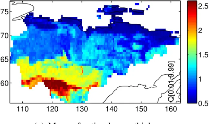
Active-layer thickness spatial patterns follow temperature patterns (Fig. 2a). Maxi-mum thaw depth in summer can be very shallow north of 70◦_{N (0.3–0.6 m) but also}

quite deep south of 65◦_{N and west of 136}◦_{E (1.5–2.7 m). Between 65}◦_{N and 70}◦_{N or}

west of 136◦_{E, ALT usually varies between 0.6 and 1.4 m. Uncertainty of ALT increases}

15

with ALT and is highest (up to 1 m) in the south (Fig. 2b). The ALT map is unique in terms of spatial extend and ALT range and therefore very useful for a comparison with global or regional models.

ALT in discontinuous and isolated permafrost zones are still not completely compa-rable to modeling results since the mapped data represents the ALT of the permafrost 20

areas within the landscape while the global model usually simulates one mean soil tem-perature profile from which ALT is further derived. Therefore, the comparison of sub-soil temperature should have higher priority in discontinuous and isolated permafrost zones.

Uncertainty, expressed as standard deviation, increases to the south because of 25

(7)

ESSDD

6, 153–162, 2013

C. Beer et al.

Title Page

Tables Figures

◭ ◮

Back Close

Full Screen / Esc

Discussion

P

a

per

|

Dis

cussion

P

a

per

|

Discussion

P

a

per

|

Discussio

n

P

a

per

4 Summary

This paper presents a map of permafrost temperature and a map of active-layer thick-ness of Yakutia, East Siberia at 0.5 degree grid cell size. A detailed scaling from 0.001 degree raster images to 0.5 degree maps using probability density approxima-tions allows a spatial mean and standard deviation that are most useful for a com-5

parison with results from land surface models which represent heat conduction and phase change. The gridded datasets can be accessed at the PANGAEA repository (doi:10.1594/PANGAEA.808240). In general, there is a strong north-south gradient of both subsoil temperature and active-layer thickness. However, mountains and soil types distributions lead to also more detailed longitudinal pattern. Uncertainties are highest 10

in mountains and in the isolated permafrost zone in the south.

References

Beer, C., Lucht, W., Gerten, D., Thonicke, K., and Schmullius, C.: Effects of soil freezing and thawing on vegetation carbon density in Siberia: A modeling analysis with the Lund-Potsdam-Jena Dynamic Global Vegetation Model (LPJ-DGVM), Global Biogeochem. Cy., 21, GB1012,

15

doi:10.1029/2006GB002760, 2007. 155

Brown, J., Hinkel, K., and Nelson, F.: The circumpolar active layer monitoring (calm) pro-gram: Research designs and initial results 1, Polar Geography, 24, 166–258, http://www. tandfonline.com/doi/abs/10.1080/10889370009377698, 2000. 155

Fedorov, A. N., Botulu, T. A., and Varlamov, S. P.: Permafrost Landscape of Yakutia,

Novosi-20

birsk: GUGK, 1989 (in Russian). 155, 156

Fedorov, A. N., Botulu, T. A., and Varlamov, S. P.: Permafrost Landscape Map of Yakutia ASSR, Scale 1:2500000., Moscow: GUGK, 1991. 155, 156

Koven, C., Friedlingstein, P., Ciais, P., Khvorostyanov, D., Krinner, G., and Tarnocai, C.: On the formation of high-latitude soil carbon stocks: E_ffects of cryoturbation and

in-25

(8)

ESSDD

6, 153–162, 2013

C. Beer et al.

Title Page

Tables Figures

◭ ◮

Back Close

Full Screen / Esc

Discussion

P

a

per

|

Dis

cussion

P

a

per

|

Discussion

P

a

per

|

Discussio

n

P

a

per

|

Lawrence, D. and Slater, A.: A projection of severe near-surface permafrost degradation during the 21st century, Geophys. Res. Lett., 32, L24401, doi:10.1029/2005GL025080, 2005. 154 Lawrence, D., Slater, A., Romanovsky, V., and Nicolsky, D.: Sensitivity of a model projection of

near-surface permafrost degradation to soil column depth and representation of soil organic matter, J. Geophys. Res., 113, F02011, doi:10.1029/2007JF000883, 2008. 155

5

McGuire, A., Wirth, C., Apps, M., Beringer, J., Clein, J., Epstein, H., Kicklighter, D., Bhatti, J., Chapin, F., de Groot, B., Efremov, D., Eugster, W., Fukuda, M., Gower, T., Hinzman, L., Huntley, B., Jia, G., Kasischke, E., Melillo, J., Romanovsky, V., Shvidenko, A., Vaganov, E., and Walker, D.: Environmental variation, vegetation distribution, carbon dynamics and water/energy exchange at high latitudes, J. Veg. Sci., 13, 301–314, 2002. 158

10

Oelke, C., Zhang, T., Serreze, M. C., and Armstrong, R. L.: Regional-scale modelling of soil freeze/thaw over the Artic drainage basin, J. Geophys. Res., 108, 4314, doi:10.1029/2002JD002722, 2003. 155

Romanovsky, V., Smith, S., and Christiansen, H.: Permafrost thermal state in the polar North-ern Hemisphere during the intNorth-ernational polar year 2007–2009: A synthesis, Permafrost

15

Periglac., 21, 106–116, doi:10.1002/ppp.689, 2010. 155

(9)

ESSDD

6, 153–162, 2013

C. Beer et al.

Title Page

Tables Figures

◭ ◮

Back Close

Full Screen / Esc

Discussion

P

a

per

|

Dis

cussion

P

a

per

|

Discussion

P

a

per

|

Discussio

n

P

a

per

Q[0.01,0.99]

110 120 130 140 150 160

60 65 70 75

−10 −8 −6 −4 −2

(a) Mean of subsoil temperature

Q[0.01,0.99]

110 120 130 140 150 160

60 65 70 75

0.5 1 1.5 2 2.5 3 3.5

(b) Standard deviation of subsoil temperature

(10)

ESSDD

6, 153–162, 2013

C. Beer et al.

Title Page

Tables Figures

◭ ◮

Back Close

Full Screen / Esc

Discussion

P

a

per

|

Dis

cussion

P

a

per

|

Discussion

P

a

per

|

Discussio

n

P

a

per

|

Q[0.01,0.99]

110 120 130 140 150 160

60 65 70 75

0.5 1 1.5 2 2.5

(a) Mean of active-leayer thickness

Q[0.01,0.99]

110 120 130 140 150 160

60 65 70 75

0.2 0.4 0.6 0.8

(b) Standard deviation of active-leayer thickness