ON THE IMPROVEMENT OF
GUILHERME AUGUSTO POTJE
ON THE IMPROVEMENT OF
THREE-DIMENSIONAL RECONSTRUCTION
FROM LARGE DATASETS
Dissertação apresentada ao Programa de Pós-Graduação em Ciência da Computação do Instituto de Ciências Exatas da Univer-sidade Federal de Minas Gerais como re-quisito parcial para a obtenção do grau de Mestre em Ciência da Computação.
Orientador: Erickson Rangel do Nascimento
Coorientador: Mario Fernando Montenegro Campos
GUILHERME AUGUSTO POTJE
ON THE IMPROVEMENT OF
THREE-DIMENSIONAL RECONSTRUCTION
FROM LARGE DATASETS
Dissertation presented to the Graduate Program in Ciência da Computação of the Universidade Federal de Minas Gerais in partial fulfillment of the requirements for the degree of Master in Ciência da Com-putação.
Advisor: Erickson Rangel do Nascimento
Co-Advisor: Mario Fernando Montenegro Campos
c
2016, Guilherme Augusto Potje. Todos os direitos reservados.
Potje, Guilherme Augusto
P863o On the improvement of three-dimensional reconstruction from large datasets / Guilherme Augusto Potje. — Belo Horizonte, 2016
xx, 67 f. : il. ; 29cm
Dissertação (mestrado) — Universidade Federal de Minas Gerais – Departamento de Ciência da
Computação
Orientador: Erickson Rangel do Nascimento
Coorientador: Mario Fernando Montenegro Campos
1. Computação. 2. Modelo digital de elevação. 3. Visão estéreo. 4. Reconstrução 3D. 5. Veículo aéreo não tripulado. I. Orientador. II. Coorientador.
III. Título.
Acknowledgments
I would like to thank to all people who somehow contributed to the development of this work, and specially to these people:
• My advisor, Erickson R. Nascimento, who guided me through this journey. He have always been very helpful and immeasurably contributed to the development of this work in every single aspect. To him I owe my deepest gratitude;
• My coadvisor Mario F. M. Campos, who undoubtedly contributed for the im-provement of this work in many ways;
• My colleague Gabriel D. Resende who worked with me in the project and made this work truly better and more complete;
• To my parents Marco and Elizabeth who always have been supportive;
• To all colleagues from VeRLab, specially Hector and Igor who worked with me on the ITV project, and Balbino who always assisted me in anything I needed in the lab.
Resumo
O advento das câmeras digitais permitiu se estimar a estrutura 3D a partir de imagens que são adquiridas por estes dispositivos de forma rápida e barata. Ao longo dos anos, inúmeras técnicas surgiram, e os algoritmos do estado-da-arte agora são capazes de prover resultados a partir de sensores de baixo custo com qualidade e resolução com-parável aos sistemas padrão da indústria. Câmeras atuais capazes de produzir imagens de alta definição são compactas, leves, e podem ser facilmente acopladas a veículos aéreos não tripulados (VANTs), em contraste a outros meios de aquisição de dados 3D, como LiDAR, que está associados a altos custos financeiros e logísticos. No entanto, o tempo de processamento das imagens coletadas rapidamente se torna proibitivo con-forme o número de imagens de entrada aumenta, exigindo hardware poderoso e dias de tempo de processamento para se gerar modelos 3D de grandes conjuntos de dados. Neste trabalho, é proposta uma abordagem eficiente baseada na técnica de estrutura a partir do movimento incremental (Structure-from-Motion) e técnicas de reconstrução estéreo para gerar automaticamente MDE - Modelos Digitais de Elevação - a partir de imagens aéreas e também modelos 3D em geral. A abordagem proposta usa a infor-mação de GPS para inicializar a estrutura de grafo usada no algoritmo, uma pontuação baseada em árvore de vocabulário para reduzir o número de pares a serem considera-dos na etapa de correspondência, uma técnica de filtragem de pontos de interesse na imagem que mantém a alta repetibilidade de pontos e reduz o custo computacional, e múltiplas otimizações locais em vez da clássica otimização global é empregado em um novo esquema para acelerar o processo incremental de estimação. Resultados obtidos com seis grandes conjuntos de imagens aéreas obtidas por VANTs e quatro conjuntos de dados terrestres mostram que a abordagem adotada supera as estratégias atuais em tempo de processamento, e também é capaz de proporcionar resultados equivalentes ou melhores em precisão comparado com três métodos do estado-da-arte.
Abstract
The advent of digital cameras heralded many possibilities of structure and shape re-covery from imagery that are quickly and inexpensively acquired by such devices. Throughout the years numerous techniques have emerged, and state-of-art algorithms are now able to deliver 3D structure acquisition results from low cost sensors with quality and resolution comparable to industry standard systems such as LIDAR and expensive photogrammetric equipments. Current imaging devices capable to produce high-definition images are compact, lightweight, and can be easily attached to un-manned aerial vehicles (UAVs), in contrast to other means of 3D data acquisition such as LiDAR, which is associated to high financial and logistical costs. However, the processing time of the collected imagery to produce a 3D model quickly becomes pro-hibitive as the number of input images increases, demanding powerful hardware and days of processing time to generate full DEMs of large datasets containing thousands of images. In this work we propose an efficient approach based on Structure-from-Motion (SfM) and Multi-view Stereo (MvS) reconstruction techniques to automatically gen-erate DEM – Digital Elevation Models – from aerial images and also 3D models in general. Our approach, which is image-based only, uses the increasingly meta-data information such as GPS in EXIF tags to initialize our graph structure, a keypoint filtering technique to maintain high repeatability of matches across pairs and reduce the matching effort, a vocabulary tree score to reduce the space search of matching and multiple local bundle adjustment refinement instead of the global optimization in a novel scheme to speed up the incremental SfM process. The results from six large aerial datasets obtained by UAVs with minimal cost and four terrestrial datasets show that our approach outperforms current strategies in processing time, and is also able to pro-vide better or at least equivalent results in accuracy compared to three state-of-the-art methods.
List of Figures
1.1 A DEM estimated from a construction site near ICEx using our approach. 7 1.2 VisualSFM graphical user interface showing a reconstructed model from
images. . . 8
2.1 Epipolar geometry between two cameras. . . 14
2.2 3-view SfM example. . . 15
2.3 An epipolar graph with 13 images from Notre Dame. . . 17
4.1 Main steps of our methodology. . . 30
4.2 Querying an image with the vocabulary tree. . . 33
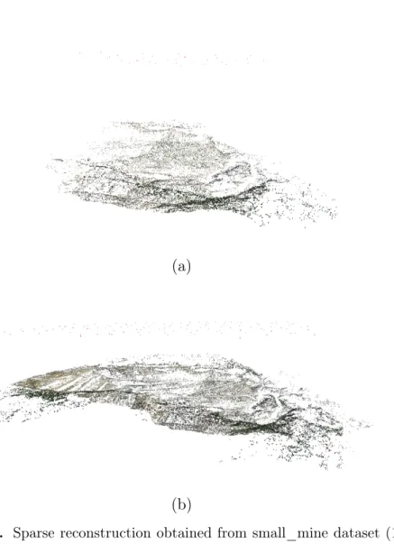
4.3 Sparse reconstruction from small_mine dataset. . . 38
4.4 Example of a simple case of the local window approach. . . 40
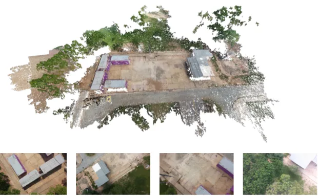
4.5 Dense reconstruction for the expopark dataset (1,231images) estimated by our method. . . 44
5.1 Image samples for each aerial dataset. . . 46
5.2 Image samples for each of the terrestrial datasets. . . 48
5.3 Mean normalized performance and error by varying the window size of the local bundle adjustment. . . 50
5.4 Time performance of each approach for the large scale datasets. . . 51
5.5 Re-projection error of each approach for the large scale datasets. . . 51
5.6 Densesurfel models estimated for the datasets. . . 55
5.7 ICEx_square after the MVS algorithm. . . 56
5.8 Quasi-dense surfel model obtained from the UFMG_Rectory dataset. . . . 57
5.9 Dense surfel model of the “Notre Dame" dataset. . . 57
5.12 Four views of the final mesh for the UFMG_statue dataset. Fine geometry details can be seen. . . 59
List of Tables
5.1 Speedup gain and mean re-projection error in pixels of the local approach compared to global BA. . . 53 5.2 Mean re-projection error in pixels when using the filtering based on the
Contents
Acknowledgments ix
Resumo xi
Abstract xiii
List of Figures xv
List of Tables xvii
1 Introduction 5
1.1 Objective and Contributions . . . 10
1.2 Thesis Organization . . . 10
2 Theoretical Background 13 2.1 Epipolar Geometry . . . 13
2.2 Structure from Motion (SfM) . . . 15
2.2.1 Epipolar Graph . . . 16
2.2.2 Bundle Adjustment . . . 16
2.3 Multi-view Stereo Algorithms (MvS) . . . 18
2.3.1 Photo-consistency . . . 19
2.3.2 Voxel-based Approaches . . . 19
2.3.3 Multiple Depth Maps . . . 20
2.3.4 Patch-based Methods . . . 20
3 Related Work 23 3.1 Structure-from-Motion . . . 23
3.2 Video-based Methods: Visual-SLAM . . . 26
4 Methodology 29
4.1 Registration . . . 29
4.1.1 Keypoint Extraction . . . 31
4.1.2 Vocabulary Tree Pruning . . . 31
4.1.3 Geometric Validation . . . 32
4.2 Filtering . . . 34
4.3 Incremental SfM . . . 35
4.3.1 Robustly Choosing The Initial Pair . . . 36
4.3.2 Robust Incremental Estimation . . . 36
4.4 Local Bundle Adjustment and Global Refinement . . . 39
4.5 Dense Reconstruction . . . 42
5 Experimental Evaluation 45 5.1 Experimental Setup . . . 45
5.1.1 Datasets . . . 45
5.1.2 Hardware . . . 47
5.1.3 Evaluation Methodology . . . 47
5.2 Parameter Tuning . . . 49
5.3 Results and Discussion . . . 50
5.3.1 Limitations . . . 54
6 Conclusion 61 6.1 Future Works . . . 62
Bibliography 63
List of Acronyms
Acronym Description
AC-RANSAC A contrario RAndom Sample Consensus
BA Bundle Adjustment
DEM Digital Elevation Model
ICP Iterative Closest Point
IMU Inertial Measurement Unit
ITV Instituto Tecnológico Vale
GPS Global Positioning System
LBA Local Bundle Adjustment
LiDAR Light Detection And Ranging
MLE Maximum Likelihood Estimator
MST Maximum Spanning Tree
MvS Multi-view Stereo
NCC Normalized Cross-Correlation
ORB Oriented Brief (Keypoint detector & descriptor)
RANSAC RANdom SAmple Consensus
RMSE Root Mean Squared Error
SfM Structure-from-Motion
SIFT Scale Invariant Feature Transform (Keypoint detector & descriptor)
SURF Speeded Up Robust Features (Keypoint detector & descriptor)
SBA Sparse Bundle Adjustment
TLS Terrestrial Laser Scanner
List of Parameters
Parameter Description
Eij Essential matrix of image pair ij
Fij Fundamental matrix of image pair ij
Ki Intrinsic calibration matrix of imagei
Pi Projection matrix of image i
coarse_inlier_rf Inlier ratio of the coarse fundamental matrix estimation step
contrast_threshold Contrast threshold used in the SIFT detector algorithm which is used to evaluate the keypoint quality.
d_nearest Amount of the closest images that are kept for each vertice in the initial graph using the GPS coordinates
k_top Amount of the biggest scaled keypoints used in the coarse estimation
for the fundamental matrix
M AX_RE Threshold in pixels to consider if a camera was correctly estimated
considering its threshold_resec
threshold_f m Inlier threshold value in pixels for the fundamental matrix estima-tion
threshold_resec Threshold value estimated for the AC-RANSAC based camera re-sectioning in pixels
τ Minimum amount of inliers a pair must have to be considered
ge-ometrically consistent in order to be present in the final epipolar graph
voc_tree_bf Branching factor of the tree used in the vocabulary tree based image
recognition approach
Chapter 1
Introduction
Geometric reconstruction of the world from a sequence of images remains one of the key-challenges in Computer Vision. Three-dimensional recovery of the geometry of an object or a scene has several applications in Computer Vision and Robotics, such as scene understanding [Li et al., 2009], object recognition and classification [Belongie et al., 2002] [Gehler and Nowozin, 2009], digital elevation mapping and autonomous navigation, to name a few.
In Robotics, 3D information is crucial to mobile robots that navigates au-tonomously in the environment, because it gives much more information about the ambient [Wurm et al., 2010]. Semantic mapping is one of the computer vision tech-niques that uses 2D-3D information to extract high-level features of the environment that can improve the agent’s decision [Henry et al., 2010].
6 Chapter 1. Introduction
at all, when there is enough baseline, overlap and texture present in the acquired images [Westoby et al., 2012].
Light Detection and Ranging (LiDAR) systems generally require accurate IMU and GPS rigidly attached and well-calibrated to obtain a global reference frame of the sensor readings, which makes the use of such approach in a campaign, expensive [Liu, 2008]. Although, recent methods based on laser [Bosse et al., 2012] are able to provide accurate 3D reconstruction results without the the requirement of GPS, and is applicable to both indoor and outdoor environments. However, LIDaR based systems are only able to measure depth and the intensity of the returned pulse, and texture information can not be directly obtained from the data.
For applications, such as aerial mapping, for instance, image-only based pipelines that incorporate recent SfM (Structure-from-Motion) and Multi-view Stereo (MvS) techniques are strong competitors to LiDAR based surface measurements [Leberl et al., 2010]. Two of the advantages of image-based reconstruction when compared to LiDAR is that several mapping tasks may also require digital images of the scene, and radio-metric information is directly registered with depth.
In particular, approaches that estimate DEMs using only images gained attention recently, specially due to the increasing availability of high quality cameras and of UAVs. Camera equipped UAVs are a low-cost and lightweight autonomous platforms that can be readily applied to acquire data processed by software packages, generating full three-dimensional models of outdoor scenes in remote areas [James and Robson, 2012]. In addition, these easy-to-use platforms can allow people with no knowledge at all in Robotics and Computer Vision to use complete image-based 3D reconstruction pipelines with minimal costs. Figure 1.1 shows a DEM estimated by our approach, and Figure 1.2 shows a sparse point cloud in VisualSFM’s graphical user interface.
A large number of techniques for recovering 3D data which describes the geometry of a scene or an environment have been proposed in the literature. In the past few years, state-of-the-art techniques in 3D photography and laser-based sensors have set the bar in accuracy in the order of a few centimeters in elevation measurement [James and Robson, 2012]. Recent methods based only on sequences of images attained significant improvements, thanks to the advancement of camera sensor technology and computer vision techniques.
7
Figure 1.1. DEM reconstructed by our pipeline followed by a sample of 4 images out of 220 used in the estimation from a construction site near ICEx. The model was obtained with minimal budget using a smartphone camera and a low-cost quadrotor.
large datasets obtained from their data stream.
A relatively new approach developed in Computer Vision field called Structure-from-Motion significantly advanced in accuracy and scalability in the past few years, and is able to retrieve the camera parameters and an initial sparse set of 3D points. Given sets of point correspondences between image pairs and the intrinsic parameters of each image, SfM pipelines are able to compute a global consistent pose (translation and orientation vector) for each image (where they were taken in the 3D space) up to an undetermined scale and an arbitrary coordinate system. Although, challenges and problems still remain unsolved. Some of the problems are that these approaches can provide wrong results when the optimization of the parameters get stuck at local minima, and the processing cost of the optimization step still is too costly. Limitations are also present, for example the lack of texture in the images makes image-based techniques useless in some cases.
8 Chapter 1. Introduction
Figure 1.2. VisualSFM [Wu, 2013] graphical user interface showing two different view points of the same reconstructed model. The colored rectangles represents the poses of the cameras in 3D. The software, which is free for research purposes, provides a friendly interface covering the complicated structure-from-motion al-gorithm, and allows people with no expertise in computer vision to use advanced techniques to estimate 3D models from images.
data. This promoted a huge advancement in 3D photography, and now it is possible to obtain 3D models without many prerequisites previously required in photogrammetry, such as structured acquisition of images, expensive and accurate GPS/IMU devices rigidly attached to the camera sensor, resulting in a costly and hard to apply approach to small and medium size mapping projects. Semi-automatic selection of point mea-surements in overlapping images were also required, increasing even more the costs [Irschara et al., 2012].
9
However, in general the processing time of SfM methods increases non-linearly with respect to the number of pictures, which makes the processing time for most real outdoor scenes, such as open-pit mines and large areas of cities, undesired, specially on consumer-grade computers. The complexity of the image registration step, which is at the core of SfM algorithms, has a time complexity of O(n2
) when using a brute force approach, where every image is tested against all the dataset to validate the geometry of a valid correspondence. Since this step is expensive in terms of processing time, naive methods already boggle down with just few hundreds of images, and become prohibitively slow when thousands of images are considered. In addition to the reg-istration step, another barrier to be overcame is the costly non-linear optimization of the camera parameters required in SfM methods called Bundle Adjustment (BA). This step is extremely important to avoid drifting during the reconstruction and provides the optimal solution for the SfM problem, being the maximum likelihood estimator for camera pose and 3D points considering that the measured points in the images have a Gaussian noise in their position.
Thus, despite the advances of SfM methods that estimate the three-dimensional structure from a sequence of images, there are still several challenges that need to be overcame to compute high quality 3D data from a large number of high definition images.
In this thesis, we combine several ideas in a novel scheme, which some of them have already proven to be efficient separately, like making use of GPS information [Frahm et al., 2010], considering only the most discriminant features of the images to make a coarse estimation of the pair geometry [Wu, 2013], the use of nearest neighbour search of the corresponding features of the valid pairs, and leveraging the
O(log(n)) complexity of the vocabulary tree search to speed up the matching phase [Nister and Stewenius, 2006]. These steps combined outperform the previously pro-posed approaches individually, and drastically reduces the time required to perform the matching step when compared to the brute force approach. Also, our proposed pipeline detailed in the methodology section is able to meticulously select image pairs with high quality of overlapping area. These steps can decrease the possibility of us-ing bad pairs in the incremental structure and motion estimation step, and drastically reduces the space search of the problem, speeding up the epipolar graph build time.
10 Chapter 1. Introduction
Therefore, as shown in Chapter 5, our approach is capable of computing the DEM faster than the other methods used in the experiments in all the tested datasets while preserving the quality of the results.
It is worth mentioning that this thesis is the result of a subproject founded by Instituto Tecnológico Vale (ITV), which is contained in a bigger context. The full idea of the project is to create a complete system that is able to map a remote area using cooperative coordination among many micro aerial vehicles and build 3D maps of the environment that also have other relevant information associated to them, e.g.
magnetic information obtained by magnetometers.
1.1
Objective and Contributions
Our goal was to develop a SfM algorithm capable of producing accurate results com-parable with the state-of-the-art SfM techniques, while focusing in time performance gains.
The general contribution of our work is the development of a new SfM pipeline that is able to deliver high quality DEMs at a low processing time cost. The main contributions can be summarized as follows:
• Proposal and implementation of a new SfM pipeline which incorporates and adapts the best techniques, both focused in time performance and accuracy, into a single algorithm;
• Proposal and implementation of an adapted overlapping local bundle adjustment window approach for large-scale datasets;
• A comparison and analysis of state-of-the-art softwares used in aerial mapping with large real world datasets acquired by UAVs.
1.2
Thesis Organization
In Chapter 2 we explore and discuss the main concepts of 3D reconstruction tech-niques, including the projective reconstruction theorem and MvS dense reconstruction techniques.
In Chapter 3 we review and detail recent state-of-the-art SfM techniques present in the literature.
1.2. Thesis Organization 11
Sequentially, Chapter 5 contains the experiments and results obtained by exhaus-tively testing seven datasets with the proposed approach and three state-of-the-art SfM implementations.
Chapter 2
Theoretical Background
In this chapter, we explore and detail important concepts and techniques used in 3D photography, which is the basis for all approaches of 3D reconstruction using collection of images.
2.1
Epipolar Geometry
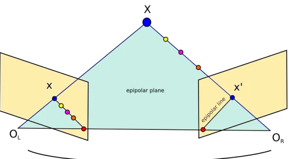
The epipolar geometry in stereo vision is the intrinsic projective geometry between two pinhole cameras that view the same static 3D scene, where the geometric rela-tions between the 3D points and their 2D perspective projecrela-tions onto the images are constrained by the camera internal parameters and their relative pose [Hartley and Zisserman, 2004].
The fundamental matrix Fij is a 3 ×3 matrix of rank 2 which describes the
geometry between a pair of images i and j according to the corresponding points that are consistent with the epipolar geometry constraint:
xTj Fijxi = 0, (2.1)
where xi and xj are the projected 2D coordinates of the same 3D point in pixels in the
images taken from different viewpoints.
14 Chapter 2. Theoretical Background
O
LO
R
X
x
x'
epip olar lineMotion and intrinsics encoded by F.
epipolar plane
Figure 2.1. Epipolar geometry between two cameras. Given the 2D coordinate
x′ in the right image, which is the perspective projection ofX onto it, the same
projection in the left image is constrained by the epipolar line, and must project along the line segment. The epipolar line of each camera can be seen as the intersection of the epipolar plane and the respective camera plane. The epipolar plane is defined by the optical center of the cameras and the 3D point, in which their 2D projections in both camera planes also lies in the epipolar plane, so this geometry does not depend on the scene structure. Note that there is an infinite number of possible epipolar lines as we moveXin the 3D space, and just one case is represented in the image.
the points by the calibration matrices or the fundamental matrix itself). We can update the fundamental matrix to the essential matrix by using the calibration matrices:
Eij=KjTFijKi, (2.2)
where Kj and Ki are the respective calibration matrices of cameras i and j. The
calibration matrix is a 2D transformation matrix in the form:
K=
fx s cx
0 fy cy
0 0 1
, (2.3)
2.2. Structure from Motion (SfM) 15
motion of the two cameras in the 3D space up to an ambiguity of scale, because we can only recover the direction of the relative translation from it.
The fundamental and essential matrix can be estimated from a set of point cor-respondences between two images (normalized image coordinates, in the case of the essential), and robust techniques like the normalized eight-point algorithm [Hartley, 1997] and the five-point algorithm [Nistér, 2004] developed in the past years allow a robust estimation from noisy image coordinates.
2.2
Structure from Motion (SfM)
In general, SfM pipelines are based on feature matching and stereo vision techniques. Recent advancements in robust feature detection and matching across images allowed the use of stereo methods that can be used to estimate the extrinsic parameters between each valid pair of cameras (sharing a portion of view in the scene) automatically. SfM core methods take as input the relative extrinsic parameters between the pairs and put
X Y Z
Relative motion =
[R|t] Global Frame P P' P'' X (3D point) Keypoint (measurement) X X X Y Y Y Z Z Z
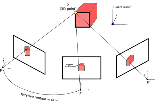
Figure 2.2. An example of the SfM problem. We want to find the projection
matrices P,P′, P′′ and X that are in the same global frame, so that we can
16 Chapter 2. Theoretical Background
them into a single reference coordinate system [Snavely et al., 2008b]. In Figure 2.2, we have a simple example of the structure-from-motion problem. Having the projection matrix for each camera relative to a global frame, it is possible to use MvS techniques to obtain a dense 3D model of the scene.
One of the most representative works that inspired numerous existing cutting-edge state-of-the-art SfM techniques until now is the well known Bundler software [Snavely et al., 2008a], which can handle a few hundred of images in a time span of days, in a consumer-grade computer. The authors used images from the Internet to create 3D models of well-known world sites, e.g. Notre Dame church, the Coliseum in Rome and the Trafalgar’s Square, obtained from social media websites.
2.2.1
Epipolar Graph
Keypoint matching is one of the most time consuming steps in a SfM pipeline. Tech-niques like ORB [Rublee et al., 2011], SURF [Bay et al., 2008] or SIFT [Lowe, 2004] and many others can be used to detect and match points across images, which requires a lot of computational effort to process high resolution photographs in the detection and description phase. In addition, the matching step, that requires comparing each descriptor of the keypoint in one image to all descriptors of all keypoints in the other to find its nearest neighbor, is also another time bottleneck in this phase, requiring
O(n2
)comparisons between high-dimension descriptor vectors to perform the match of two images optimally, considering thatn is the number of keypoints in the images.
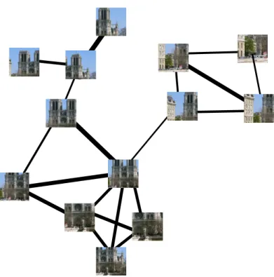
The epipolar graph is widely used to represent the geometric relation between each pair of image in the scene and can be defined as follows: G = (V,E), where each vertex v ∈ V represents an image and there is an edge e ∈ E between two vertices if there is a valid epipolar geometry relation between the images which is described by the fundamental or essential matrix. A simple epipolar graph is shown in Figure 2.3.
In the naïve approach, each image is matched against all other images in the dataset using a brute force nearest neighbor search for each possible pair to attribute the correspondence for each point, and then RANSAC [Fischler and Bolles, 1981] is used to robustly estimate the essential matrix between each pair, as also to remove the outliers from the correspondences.
2.2.2
Bundle Adjustment
2.2. Structure from Motion (SfM) 17
Figure 2.3. An epipolar graph with 13 images from Notre Dame. The thickness
of the edges indicates a higher number of correspondences between pairs.
all approaches with no exception, to reduce drifting and improve accuracy. Once new camera poses are estimated and their 2D features are triangulated into 3D points, there is a need to optimize these estimated parameters due to estimation errors which accumulates in the model. The optimal solution for this problem considering Gaussian noise in the position of the keypoints, is the maximum likelihood estimator (MLE).
In this optimization problem, we want to estimate the camera poses and 3D points that minimizes the squared re-projection error in pixels between the measured and predicted projections. Considering that each camera pose j is parameterized by a projection matrix Pj and each 3D pointiby a vectorXi, we can write the optimization
problem as minimizing:
min
Pj,Xi
X
i=1 X
j=1
kXiPj−xij k
2
, (2.4)
18 Chapter 2. Theoretical Background
Considering that the parameters of each projection matrix has 6degrees of free-dom (three for the position and three for orientation) and each 3D point has3degrees of freedom (X,Y and Z coordinates), the total dimensions of the problem to solve can be calculated as6j+ 3iin this case. Other parameters as focal length, principal point and distortion coefficients can also be considered in the optimization, increasing even more the number of parameters of each camera. For large datasets, such as the ones containing thousands of cameras and millions of 3D points, the dimensionality of the problem is extremely high, and minimizing its cost function demands highly specialized algorithms that need to be extremely efficient and well-implemented.
In spite of the efforts of the community and the improvements already made, specially in exploiting the sparse block structure that arises in bundle adjustment to speed up the computation [Lourakis and Argyros, 2009], the problem is still costly to solve for large datasets. However, Eudes and Lhuillier [2009] shows that using a local bundle adjustment instead performing a global optimization in the incremental process on video-based reconstructions can achieve good quality results and provides a considerable speed up gain. Another solution for this problem is to use a divide-and-conquer approach [Ni et al., 2007], which can also accelerate the optimization while maintaining good accuracy relative to global bundle adjustment.
2.3
Multi-view Stereo Algorithms (MvS)
Multi-view stereo algorithms take as input fully calibrated intrinsic and extrinsic cam-era parameters and their respective images, and gencam-erate aquasi-dense 3D model based on correspondences between images. They can be roughly classified into four classes according to the underlying object models, being them shape-from-sillouetes, voxel-based, patch-based and graph-based. Each of them has its limitations, specially for considering some assumptions that are not general for every scenario. This limits the dataset type a technique can be applied, being them object and scene datasets.
2.3. Multi-view Stereo Algorithms (MvS) 19
2.3.1
Photo-consistency
Photo-consistency tests are widely used in the techniques described below. Such tests are based on color or greyscale variance information that can be used as constraints in 3D reconstruction as a valid three-dimensional point in a world’s surface as it’s projection onto the visible cameras will theoretically have the same intensity or color, considering small variations of illumination and Lambertian reflectance. One of the most used scores to measure the similarity of patches in images is the normalized cross-correlation, which is given by the formula:
N CC = 1
n
X
x,y
(f(x, y)−µf)(t(x, y)−µt)
σfσt
, (2.5)
where f and t are two corresponding patches in the images, n the total amount of pixels in the patches, and σ and µthe respective standard deviation and mean of the patch. A fixed threshold is usually set, and patches are declared inconsistent if they are not similar enough.
2.3.2
Voxel-based Approaches
In voxel-based approaches, a bounding box containing the volume of the scene is ini-tialized, and every unit of this volume is formed by avoxel. We can do a direct analogy of voxels as being 3D pixels, like we have pixels in ordinary images. They have 3D coordinates and a color, like a pixel in an image has 2D coordinates and also a color. But this limits the technique, because there is a need to know a valid volume containing the scene, limiting the technique to object datasets only, and the quality of the model as also the computational cost is dependent of the resolution of the voxel space. Then, an iteration is made to verify the photo-consistency of the voxel, achieved by project-ing the voxel onto all camera planes that can see it, and color variance is analyzed to determine if the voxel is photo-consistent or not. In case it is not, it is removed from the volume space.
20 Chapter 2. Theoretical Background
houette information has not enough information to converge into the real shape of the object, depending on the shape of it, even when there is a possibility to obtain infinite number of images of the object in all possible poses. Another limiting factors of shape-from-silhouettes techniques are the number of images necessary to provide a good approximation of the shape, and also the pose of the cameras of the images. If there is too few images available, or a bad distributed viewpoints of the object, these kind of approaches can provide very rough results. A method presented by Shanmukh and Pujari [1991] considers some prior knowledge of the object shape and provides a solution that optimises the reconstruction specifying the viewpoints necessary.
2.3.3
Multiple Depth Maps
These techniques rely on estimated depth maps for each pair of image. Once the depth maps are obtained using stereo algorithms, they are merged onto a single model. These kind of techniques are simple and more flexible but requires many well-distributed views of the object to achieve good results. An example of the power of this technique, Irschara et al. [2012] developed a full methodology to obtain a dense model from large scale and highly overlapping aerial images. The core component of the approach is a multi-view dense matching algorithm that explores the redundancy of the data. A multi-view plane sweep technique is applied to perform the match, where the 3D space is iteratively traversed by parallel planes which is usually aligned with a particular key view. For each depth in the plane, sensor images are projected onto the plane and a similarity function is used to compute a cost. After, a depth map can be extracted using a minimum graph cut algorithm. The final result of the approach is a model with depth value estimated for every possible pixel in the images.
2.3.4
Patch-based Methods
Being one of the most flexible techniques, patch-based approaches can achieve good re-sults in the majority of datasets (objects and scenes), except in texture-less or occluded regions. These approaches first generate a set of sparse 3D oriented points using feature matching correspondences across images, and then iteratively expand these patches to increase density.
2.3. Multi-view Stereo Algorithms (MvS) 21
Chapter 3
Related Work
In this chapter, we discuss relevant methods present in the literature that try to solve the Structure-from-Motion problem, pointing out the advantages and disadvantages of each one.
3.1
Structure-from-Motion
Incremental SfM reconstruction techniques aim at solving the problem incrementally. Our method fits in this category, being an extended pipeline, that is, in the end of the pipeline we also have the dense reconstruction and the estimated mesh with the projected textures.
Incremental SfM approaches are able to handle unordered collection of images. In other words, they do not make any assumption of temporal sequence in the frames, do not require high redundancy of images, and do not rely in any loop closing technique, since the feature tracking among cameras occurs globally considering the entire dataset. Such scheme allows SfM techniques to be robust, accurate and near-optimal in most cases after global bundle adjustment, although it might get stuck at a local minima eventually.
24 Chapter 3. Related Work
the ones obtained on the Internet or datasets commonly gathered by inexperienced people.
Bundler [Snavely et al., 2008a] is based on incremental SfM. First, features and meta-data are extracted for each image, and then an exhaustive brute-force matching of features is performed between each possible pair. Then, the fundamental matrix is estimated and finally the incremental reconstruction is performed by adding new cameras in a greedy manner through camera resectioning and triangulating new points with the before estimated cameras. The major drawback of the approach is the number of images that can be used for the reconstruction, which is bounded to a few hundreds, since the time required to process more than that rapidly becomes prohibitive due to both brute-force matching and multiple global BA calls that are required during the reconstruction. In the end, the pipeline provides the projection matrices for the images and a sparse point cloud.
The method of Frahm et al. [2010] is applicable to the structure and motion estimation of large-scale datasets. To deal with the high redundancy of images from image queries from the internet, they first clusterize the images and for each cluster they consider just an iconic image. Then, a result retrieved from a vocabulary tree search is used to perform the feature matching and geometry validation of thek closest images to the query image defined by a similarity score, giving a huge speed up of the epipolar graph building. However, their method tends to reconstruct unconnected clusters consisted of subsets of the original dataset.
The geo-location occasionally available can also be exploited to deal with the problem of fragmented models generated by large-scale SfM. Strecha et al. [2010] lever-age the geo-location available, among other meta-data (DEMs and 2D building models), to deal with the fragmentation problem and also allow the update of the estimations when new images of the region become available without the necessity of redoing the process from scratch. But the method depends on reliable information to generate good results, such as accurate GPS.
3.1. Structure-from-Motion 25
meta-data to compute a coarse projection matrix for each camera using the available GPS and IMU data. By means of a pre-existing 3D model of the scene or making weak assumptions on its maximum depth, the method is able to estimate a coarse overlap between the images. Thus the feature match process occurs among the ones with overlapping views, improving significantly the time performance compared to the brute-force matching and avoiding ambiguity. However, IMU data and pre-existing models are not commonly available, limiting the applicability of this technique.
In order to overcome the costly matching step, the work of Wu [2013] tries to reduce the time consumption by using approximate nearest neighbor search and care-fully selecting subsets of keypoints to be matched. For a moderate number of images (few hundreds), this approach is efficient, but it does not avoid the quadratic complex-ity of matching. The authors also use preconditioned conjugated gradient which can accelerate the convergence of the optimization in the bundle adjustment step. Further-more, they explore the pleasingly parallelizable characteristics of the problem to speed up the process by using multi-core processors and GPUs. The results remain as one of the state-of-art techniques, although for very large datasets, the method requires powerful hardware, such as multiple GPUs and many threads to provide the solution in acceptable time.
Other works focused at improving bundle adjustment, which is an essential part of the SfM pipeline, thus, receiving intense research in the past years. Jeong et al. [2012] perform experiments with several bundle adjustment methods present in the literature, and proposes two methods that work in the reduced camera system that leverages the natural block sparsity. While one is based in exact minimum degree ordering and block-based LDL (lower triangular and diagonal matrix decomposition) solving, the other uses a block-based preconditioned conjugate gradient. The reported results show that the methods are able to converge faster, in addition to handle memory efficiently. However, the strategies for the linear solvers were not fully investigated as pointed by the authors, and better results can be achieved with a proper investigation.
26 Chapter 3. Related Work
3.2
Video-based Methods: Visual-SLAM
Video-based methods, also known as Visual-SLAM, use similar stereo techniques to estimate the relative camera poses, but differently from the structure-from-motion for unordered collection of images, they use the temporal relation between the frames to skip the matching step. Using fast tracking techniques such as optical flow, the points are tracked in the most recent frames of a video stream, which requires a high frame-rate to maintain the relative change of frames very low. Generally, the images resolution are limited by these techniques if one wants to achieve real-time performance.
Because these methods aim at running in real-time, global bundle adjustment is undesirable at any point, and the uncertainty of the camera poses in long sequences is high. Consequently, they rely on loop-closure techniques to attempt drift correction on-the-fly, however, loop detection may be too expensive for large datasets and does not guarantee that all loops will be detected. Furthermore, the 3D model generated by these techniques can suffer from multiple estimations of the same 3D point, because they only keep track of the most recent features in the images, providing a sub-optimal solution which may lead to reduced global accuracy specially on large datasets.
Thus, these techniques are not usually used to estimate 3D models in general because of their limitation in accuracy, but they are commonly used in robotics to provide a coarse estimation of the robot’s pose and the environment structure in 3D using low-cost cameras, being very useful in that case.
Pollefeys et al. [2008] proposed a real-time system that is able to deliver dense 3D information from a video stream of an urban area. They rely on accurate INS and GPS to provide the camera poses. Eight cameras were positioned in different points of view attached to a vehicle, and then a calibration was performed to compensate the difference of coordinate system of the cameras and the INS/GPS sensors. Using the camera poses provided by the sensors, a subset of frames with sufficient baseline are constantly selected, and a GPU implementation of the plane sweep algorithm originally proposed by Collins [1996] is used to achieve real-time 3D depth estimation.
3.3. Structure-from-Motion versus LiDAR 27
one wants to achieve real-time results running in CPU. The technique also suffers from pose drifting for long sequence of frames, specially if no loop is found.
3.3
Structure-from-Motion versus LiDAR
The work of James and Robson [2012] applies a 3D photography methodology to geo-sciences. By using SfM and multi-view stereo (MVS) techniques, the authors generate models and compare them against laser scanned models. A consumer-grade camera, low cost UAVs and computer vision software were used in the experiments, and they concluded that the combination SfM+MVS is capable of producing useful 3D models with a decrease of 80% in the total time spent in a mapping campaign (considering the logistics until the final result) in comparison to LiDAR. Similarly, the work of Westoby et al. [2012] presents a survey concluding that 3D photo techniques are good options to produce topographic data in an efficient cost and low-time way, in contrast to the traditional surveying campaigns using lasers and manned aerial vehicles, which require high financial and logistical costs, and demand specialists to perform the data acquisition.
More recently, the work of Micheletti et al. [2015] demonstrates that even an ordinary smartphone camera with5.0megapixel resolution processed by a SfM pipeline is able to deliver satisfying results. The authors compare the models generated by SfM against those generated by a well established photogrammetric software and LiDAR. Their results reinforce that SfM approaches are a fully automated and inexpensive way to obtain reliable 3D information.
dis-28 Chapter 3. Related Work
night survey are required , while the TLS is partially suitable for these tasks.
Chapter 4
Methodology
In this section we detail the main steps of our methodology. It is a novel pipeline that provides two new features: An efficient epipolar graph building procedure and a local bundle adjustment adapted to large-scale reconstructions.
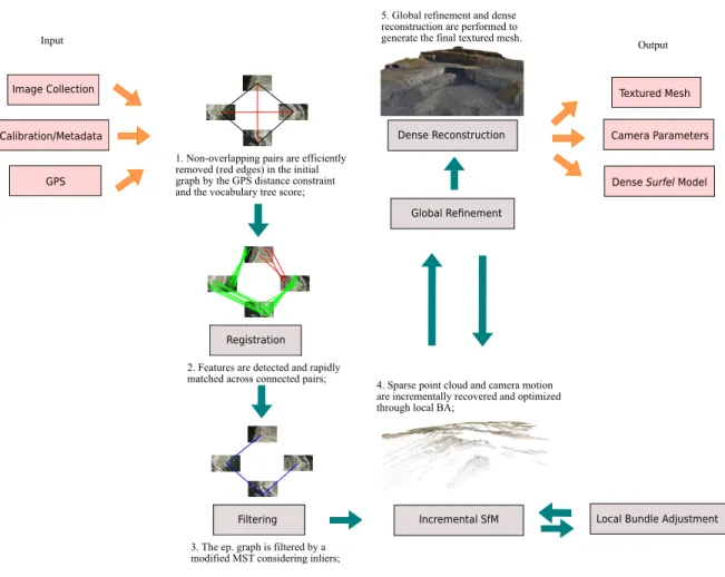
First, the GPS constraint in addition to the vocabulary tree score are used to efficiently prune non-overlapping pairs (Figure 4.1– I) followed by a coarse to fine geometry validation to save even more processing time in the feature matching phase (Figure 4.1– II). The epipolar graph’s edges are then updated by the modifed maximum spanning tree algorithm (Algorithm 2) that carefully selects the best ones to be used in estimation of the camera parameters and the scene structure while enforcing the completeness of the graph (Figure 4.1– III). The camera motion and intrinsics, as well the 3D structure parameters are locally optimized by an overlapping window containing the most recent cameras (Figure 4.1– IV). As a direct consequence of using the proposed local bundle adjustment (LBA), our approach demands less global optimizations to provide an accurate solution in the end of the reconstruction. In the final step, our pipeline computes the dense model using a patch-based multi-view-stereo technique and Poisson reconstruction to obtain the final mesh (Figure 4.1– V).
4.1
Registration
30 Chapter 4. Methodology
Image Collection
Filtering Incremental SfM
Dense Reconstruction
GPS
Local Bundle Adjustment Global Refinement
1. Non-overlapping pairs are efficiently removed (red edges) in the initial graph by the GPS distance constraint and the vocabulary tree score;
3. The ep. graph is filtered by a modified MST considering inliers;
4. Sparse point cloud and camera motion are incrementally recovered and optimized through local BA;
5. Global refinement and dense reconstruction are performed to generate the final textured mesh.
Calibration/Metadata
Input
Textured Mesh
Output
Camera Parameters
DenseSurfelModel
Registration
2. Features are detected and rapidly matched across connected pairs;
Figure 4.1. Illustration of the main steps of our methodology. We initialize
the epipolar graph by connecting images with a large chance of having overlap, according to GPS data and a vocabulary tree search. In this example, the black edges are below the threshold distance, and the vocabulary tree query of at least one of the images are among the top 40 highest score matches of the other, so they are kept while the red ones are removed. After the optimized pairwise regis-tration, we update the epipolar graph by selecting high quality matches enforcing completeness, here represented by the blue edges in step III. The camera mo-tion is incrementally recovered for each image and a sparse point cloud generated from the matching points and optimized through robust and fast local bundle adjustment. At the end, we compute the dense model.
distance between the position of image pairs is large, they do not share any portion of view. By considering that, we generate an initial graphG = (V,E), where each vertex
v ∈ Vrepresents an image. We connect thed_nearestimages according to the distance obtained by compairing each pairs’ GPS coordinates. We usedd_nearest= 40 in our experiments, which is a sufficient value for all datasets in our experiments. Reducing this value can reduce even more the effort of matching although it can prune pairs that overlap.
complex-4.1. Registration 31
ity of matching n images from O(n2
) to O(n) considering aerial and large datasets. Additionally, this avoids comparing ambiguous pairs, which makes the approach more robust to wrong reconstructions due to views that are actually geometrically consistent but are not viewing the same portion of the scene (e.g. symmetric building facades).
4.1.1
Keypoint Extraction
In general, SfM techniques look for the correspondences between images to estimate the camera extrinsic parameters and to generate the final sparse three-dimensional point cloud. We used SIFT [Lowe, 2004] to extract the keypoints and compute their descriptors due to its good invariance to scale and affine transformations that occur, as a consequence of cameras looking at the same region in many different viewpoints.
To avoid that too many keypoints are considered by our approach which is bad both due to ambiguity and unnecessary elevated processing time to match and optimize in the SfM phase, we sort the found keypoints by descending order of scale and remove the small keypoints so that we keep the features with large scale attribute up to 9.000
features per image, which is a sufficient amount of keypoints for the most scenarios, as suggested by [Wu, 2013]. The reason we select the features with large scale attribute in many steps in the approach is because they have a higher repeatability rate than small scale features and their descriptors tend to be more discriminant.
4.1.2
Vocabulary Tree Pruning
In some cases, the GPS tags are missing for some images, and it can become a problem when a dataset has most of its images without GPS information. Thus, we cannot remove the edges of the respective vertices that correspond to those images because we do not have any prior information to infer if the pairs overlap. Depending on the size of the dataset, it can cause a strong negative impact in the processing time of this phase.
To overcome this problem, we use a vocabulary tree approach similar to Nister and Stewenius [2006] to avoid theO(n2
)time complexity in the matching step. Vocabulary trees are used in scalable image recognition, where similar images are returned by a recursive search in the tree given an image query (the search term). The algorithm we used to build a vocabulary tree can bee seen in Algorithm 1. Using the SIFT descriptors, we build a vocabulary tree with a branching factor (voc_tree_bf) of 9
32 Chapter 4. Methodology
in each image selected uniformly. We finally index the tree leafs using the top 3000
features (ordered from large to small scale value) of each image. Once the tree is indexed, we can query an image for images with close visual appearance to it, taking
O(log(n)) time complexity in a balanced tree, where n is the number of images in the entire dataset. These parameters were varied in our experiments, and we concluded that selecting 600 random keypoints produce a varied set of features and reduces the memory usage to build the tree, and querying for the 3000 largest features produces improved matching results rather than querying for the entire set, mostly because the largest features are more stable. The visual similarity score for each image is obtained by propagating again the 3000 features with largest scale attributes. The algorithm increments the bin’s score of the respective indexes of the images that are present in the leaf of each descriptor propagation in the histogram of indexes for the image query. We have used the increment score as being:
score= 1
nl, (4.1)
where nl is the node level, so the most common features will contribute less to the score of the bins that are indexed in the leaf. Intuitively, the most common features will have larger clusters and the depth of the path for these less discriminant features will be larger.
In our experiments, we search for the top 60 highest score matches for each image (the most similar ones to that query according to the vocabulary tree), and we prune the edges in the epipolar graph from the query vertice to those vertices that are not among the highest scores of this query, excepting the edges that were validated by the GPS distance. The time complexity cost of the entire pruning operation isO(nlog(n)), being n the number of images. Here, we consider that the tree is balanced assuming that the keypoint descriptors we used to build the tree were randomly chosen, even though it may not be true if there are too many similar features in the images. This approach enforces the matching step to be linear in time since each image will have at most 60candidates to perform the registration.
4.1.3
Geometric Validation
After the graph construction, we can efficiently match image pairs in a reduced space search, which initially hadO(n2
4.1. Registration 33
c
c
c Feature Space in the last level of the path
Upper Node
F
...
[3,7,1] [2] [0,5,8,9]
0 1 0 1 0 0 0 1 0 0 Histogram:
Image query (1 out of 3.000 features...)
Leafs c c c
F
0 1 2 3 4 5 6 7 8 9
Figure 4.2. Example of a query for an image. The first feature is being prop-agated down. In this case, the branching factor of the tree is three, and in each level, the feature is compared to the three node centers and it is propagated to the one that is the closest to it. The process is recursively done until it reaches a leaf, where the histogram is incremented with the score (1 in this case for simplicity)
for each respective index the leaf holds.
Algorithm 1 Vocabulary tree building.
procedure BuildVocabularyTree(N ode,F eatureSet,BranchingF actor) Cset = K-means(F eatureSet, BranchingF actor)
for eachcluster C and its respective child node do
SetChildCenter(ChildN ode, Center(C)) if Size(C)>5×BranchingF actor then
BuildVocabularyTree(ChildN ode, C,BranchingF actor) ⊲
Recursively divides the feature space into nVoronoi cells, wheren is the branching factor.
two small sets containing the biggest (most discriminant) keypoints of their respective images, selected according to the scale attribute. If the correspondences are able to minimally satisfy the epipolar geometry constraint, a full pairwise match considering all keypoints are performed to obtain a fine pairwise registration.
34 Chapter 4. Methodology
pairs of keypoints do not provide a valid epipolar geometry, we remove the edge of the graph. We consider a pair as valid if the number of inlier correspondences returned by the fundamental matrix estimation 2.1 using RANSAC [Fischler and Bolles, 1981] is higher than at least 15% of the number of matches between each pair, which we callcoarse_inlier_rf. The 15%value was chosen by performing tests on image pairs and we concluded when there is less than 15% of inliers in the correspondences using
k_top = 600, the likelihood of overlap between them is minimal. These steps are performed only between images that are connected in our graph. To avoid requiring the intrinsics for the images, we use the fundamental matrix in this step instead of the essential matrix, since for some images the intrinsics may not be available or have incorrect parameters.
Fine Pairwise Registration: To perform the fine registration, we fully match the keypoints between image pairs that have passed in the fast geometry validation. We now use all the keypoints found in both images with Fast Approximate Nearest Neigh-bour search (FLANN) [Muja and Lowe, 2009]. We also use the ratio test criterion, discarding similar distances of the two nearest neighbours of a query descriptor. We use a ratio of0.8in our experiments, which is the suggested value in the original SIFT paper [Lowe, 2004]. This step filters out ambiguous pair matches which have a higher chance to be wrong correspondences and decreases the set of points to be considered by the RANSAC. By doing that we also raise the probability of finding a valid pairwise geometric estimation (fundamental matrix), since the ratio ofinliers/total in the set of correspondences is increased. At last, we estimate the fundamental matrix by using the RANSAC scheme with the normalized 8-point algorithm [Hartley, 1997] to validate a pair geometry. Again, we use the fundamental matrix to avoid using wrong intrinsics. A threshold in pixel is defined (threshold_f m = 0.07% of the image width in our tests) to determine if the point is an inlier or not, depending on the distance that it is from the respective epipolar line in the other image, which is a similar threshold used by Bundler [Snavely et al., 2008a], and were tested many different datasets.
4.2
Filtering
4.3. Incremental SfM 35
difficult to define a hard threshold for this purpose, depending on many factors, e.g.
matching quality, amount of texture in the images and overlap. Therefore, we propose applying a maximum spanning tree approach (MST) to remove only the edges with small number of inliers but enforcing the connectivity of the graph, since the MST avoids us breaking the epipolar graph into smaller connected components when we try to remove an edge with low number of inliers.
The last step of the epipolar filtering consists in extracting the sub-graph that contains the edges from the maximum spanning tree and the edges with the number of inliers larger than a defined thresholdτi(we use a value of60inliers in our experiments, a standard value used by Bundler [Snavely et al., 2008a] and VisualSFM [Wu, 2013]).
This procedure is described by the Algorithm 2. The complexity of the Algo-rithm 2 lies in the same of Kruskal’s algoAlgo-rithm O(elog(e)) since only an additional
O(e) iteration is required.
4.3
Incremental SfM
Our methodology uses an incremental structure-from-motion approach. The algorithm begins the reconstruction by using a pair of images and then incrementally estimate the points and cameras parameters, adding them to the model sequentially. The camera motion estimation happens in a greedy manner with respect to the number of 2D-3D correspondences. In other words, the method estimates the camera motion through resectioning by choosing the camera that provides the largest amount of 2D-3D corre-spondences and then triangulates new 3D points into the model, until there is no more cameras to add.
Algorithm 2 Epipolar graph filtering.
procedure EpipolarFiltering(EG, τi)
MaxSpanningTree(EG, F ilteredEG) for eachedge e in EG do
if weight > τi & e /∈F ilteredEG then
Add(F ilteredEG, e) returnF ilteredEG
36 Chapter 4. Methodology
4.3.1
Robustly Choosing The Initial Pair
Choosing the initial pair is crucial to the quality of the reconstruction. If we choose a pair not having enough overlap, the reconstruction can fail immediately. But if we also choose a pair that have almost no translation motion (generally, they will overlap almost entirely), the essential matrix estimation and initial triangulated points will be ill-conditioned, because there is not enough parallax for the algorithm to infer the depth of the scene. To avoid that, we sort the edges of the graph and keep a percentile of 0.4 of the most valued edges (this value is arbitrary and is not sensitive when it is not set on the extremes like ≤ 0.10 or ≥ 0.90 according to our experiments), which contains consistent geometric pairs that undoubtedly overlap. Then, we sort this subset considering the ratio between the essential matrix inliers and the homography inliers and use a percentile of0.25(again, the percentile value is not sensitive and is arbitrary) of the subset containing the highest ratio between the fundamental matrix inliers and homography inliers (Finliers/Hinliers), which is useful to avoid the use of small-baseline pairs in the seed reconstruction. Homographies cannot explain parallax in the scene, just the motion of planar surfaces. The number of homography inliers then will be, in general, lower than the inliers of the fundamental matrix for pairs with sufficient translation motion, except in the case when the entire scene is planar, which is fair to assume that is not in our context.
We then finally select the pair which provide the lowest mean re-projection error in this small subset of candidates. The essential matrix (2.2) is estimated using the normalized camera coordinates of the correspondences, calculated using the respective camera intrinsic parameters extracted from the EXIF meta-data or a calibration file. To perform the reconstruction of the initial pair, there must exist some source of information of the intrinsic parameters, or it will not be possible to approximately estimate the relative euclidean motion for them. An initial point cloud is created by triangulating the feature correspondences using the relative euclidean motion extracted from the essential matrix and refined using bundle adjustment.
4.3.2
Robust Incremental Estimation
From the initial point cloud, we find the image with the largest 2D correspondences with 3D points already estimated and we calculate the extrinsic parameters from the camera through camera resectioning. Camera resection techniques uses the 2D-3D correspondences to find a projection matrix Pi that maximizes the number of inliers
4.3. Incremental SfM 37
approach of Moulon et al. [2013] that uses ana contrario RANSAC scheme for solving for Pi, where an inlier threshold is also estimated. The threshold choice for a pure
RANSAC scheme for estimating Pi is usually done empirically and do not generalize
well for different kind of datasets.
We first estimate a normalized Pi using normalized image coordinates, and
then we evaluate the ratio of inliers and the threshold estimated. If the inlier ra-tio inlier/total is fewer than 0.25 or the threshold is above 24.0 pixels (M AX_RE), we assume that the intrinsic parameters of the camera are wrong. The values of these paramaters are similar to Bundler and works well for all datasets we tested. We then try to re-estimate the unnormalized Pi and decompose it into two matrices using the
RQ decomposition. The two matrices are actually the rotation matrix (an orthogonal matrix) and the calibration matrix Ki of camerai. Finally, we are able to extract the
new focal length fromKi, and re-estimate the normalizedPi. If the camera resectioning
fails again, we exclude it from the model.
If a valid estimate of Pi is obtained, our algorithm optimizes the camera
param-eters including the focal length and camera distortion through a single-camera bundle
Algorithm 3 Incremental estimation.
procedure IncrementalSfM(Structure,Cameras, EG) while NotAllChecked(Cameras)do
BC ← FindBestCamera(Structure, Cameras)
ResectionNormalized(Structure, BC)
if BC.InlierRatio <0.25∨BC.threshold_resec > M AX_RE then
ResectionUnnormalized(Structure, BC)
UpdateFocalLength(BC)
ResectionNormalized(Structure,BC)
if BC.InlierRatio <0.25∨BC.threshold_resec > M AX_RE then
continue ⊲Skip this camera.
else
OneCameraBundleAdjustment(BC)
TriangulatePoints(Structure, BC, Cameras, EG) else
OneCameraBundleAdjustment(BC)
TriangulatePoints(Structure, BC,Cameras, EG) ⊲Triangulate points with connected cameras in the graph that have already been estimated.
if N umberOf EstimatedCameras mod window_size= 0 then
LocalBundleAdjustment(Structure, Cameras)
GlobalBundleAdjustment(Structure, Cameras) ⊲
38 Chapter 4. Methodology
(a)
(b)
Figure 4.3. Sparse reconstruction obtained from small_mine dataset (127
im-ages) during the incremental estimation of the camera parameters and sparse 3D structure. (a) Partially reconstructed model (32 images); (b) Fully reconstructed
model.
adjustment with fixed 3D points. Finally, we triangulate the points that are not in the model by visiting the connected estimated cameras using the epipolar graph. We discard the points with a triangulation angle smaller than2.0degrees (a standard value used in many stereo algorithms, such as [Furukawa and Ponce, 2010], [Snavely et al., 2008a], [Wu, 2013]) because the cameras do not have enough baseline to provide a good estimation of the 3D intersection.
4.4. Local Bundle Adjustment and Global Refinement 39
in Figure 4.3. Algorithm 3 shows the incremental estimation procedure.
4.4
Local Bundle Adjustment and Global
Refinement
Bundle adjustment (BA) techniques attempt to minimize the re-projection error be-tween the observed and predicted image points in order to obtain the optimal 3D structure and camera parameters (Subsection 2.2.2).
Due to the large number of unknown parameters which contributes to the re-projection error value, a standard implementation of this optimization method would have massive computational costs when applied to the minimization problem charac-terized in bundle adjustment. Lourakis and Argyros [2009] proposed a method that explores the sparse block structure of the non-linear optimization problem in BA con-text achieving a considerable time performance gain (Equation 4.5).
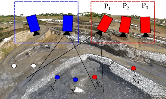
However, finding the optimal solution for this problem is still time consuming when considering thousands of cameras and millions of 3D points. To tackle with this problem, we propose an overlapping local bundle adjustment window approach that optimizes the camera poses and points locally, but it overlaps with already optimized 3D points to hold the consistency and avoid fast propagation of drifting. Although this approach can be find in several video-based (i.e. small baseline and organized dataset) methods, in our work we apply this approach for unorganized dataset of large baselines.
Let V = (P1, . . . , Pm, X1, . . . , Xn)T be a vector containing all
parame-ters describing the m projection matrices and the n 3D points, and X = (xT
11, . . . , x
T
1m, . . . , xTn1, . . . , x
T
nm)T the measured image point coordinates across the cam-eras (position of the detected keypoints). By using the parameter vector, we can create the estimated measure matrix as:
ˆ
X= (ˆxT11, . . . ,xˆ
T
1m, . . . ,xˆ
T
n1, . . . ,xˆ
T nm)
T
, (4.2)
where xˆT
ij is the projection of the 3D pointi in the camera j.
We can write the BA as the optimization problem of finding the values that minimize:
(X−Xˆ)TΣ−1
X (X−Xˆ) (4.3)
40 Chapter 4. Methodology
P
1
P
2P
3X
1X
2X
3X
4Figure 4.4. A simple case of the local window approach. The blue selection
represents the points and cameras that have already been bundle adjusted, while the red selection will be optimized when the window becomes full. The green points will contribute to the minimized re-projection error of the cameras, but since they already are optimized, their parameters will remain fixed.
mented weighted normal equations:
(JTΣ−1
X J+µJ)δ=J
TΣ−1
X (X−Xˆ), (4.4)
where J represents the Jacobian of Xˆ, δ the update parameter of V that we are estimating and µis the damping term which is used to change the diagonal elements of the Jacobian.
4.4. Local Bundle Adjustment and Global Refinement 41
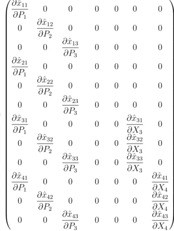
Figure 4.4, the Jacobian J can be write as:
J=
∂xˆ11
∂P1
0 0 0 0 0 0
0 ∂xˆ12
∂P2
0 0 0 0 0
0 0 ∂xˆ13
∂P3
0 0 0 0
∂xˆ21
∂P1
0 0 0 0 0 0
0 ∂xˆ22
∂P2
0 0 0 0 0
0 0 ∂xˆ23
∂P3
0 0 0 0
∂xˆ31
∂P1
0 0 0 0 ∂xˆ31
∂X3
0 0 ∂xˆ32
∂P2
0 0 0 ∂xˆ32
∂X3
0 0 0 ∂xˆ33
∂P3
0 0 ∂xˆ33
∂X3
0
∂xˆ41
∂P1
0 0 0 0 0 ∂xˆ41
∂X4
0 ∂xˆ42
∂P2
0 0 0 0 ∂xˆ42
∂X4
0 0 ∂xˆ43
∂P3
0 0 0 ∂xˆ43
∂X4 . (4.5)
In our implementation, we first used the Sparse Bundle Adjustment (SBA) library as the optimizer solver [Lourakis and Argyros, 2009], but then we verified that there is a newer, more efficient and flexible implementation of a non-linear least squares solver called Ceres [Agarwal et al., 2015] that also leverages the sparse structure of the Jacobian, which we later used to model and optimize the parameters of our SfM problem in a very practical way, and it was able to provide slightly better re-projection error results.
The incremental approach estimates camera motion and scene structure calling bundle adjustment multiple times. As the number of parameters of the model incre-mentally increases, the time to perform a global BA iteration rapidly grows with the number of cameras and points. Our approach proposes to fasten the parameters of the 3D points that have already been bundle adjusted and only adjusts the parameters of the newest estimated cameras and points.
The time complexity of bundle adjustment considering the sparse block structure is O(m3
![Figure 1.2. VisualSFM [Wu, 2013] graphical user interface showing two different view points of the same reconstructed model](https://thumb-eu.123doks.com/thumbv2/123dok_br/15649717.620349/28.892.210.657.119.591/figure-visualsfm-graphical-interface-showing-different-points-reconstructed.webp)