CENTRO DE TECNOLOGIA
DEPARTAMENTO DE ENGENHARIA DE TELEINFORMÁTICA
PROGRAMA DE PÓS-GRADUAÇÃO EM ENGENHARIA DE TELEINFORMÁTICA DOUTORADO EM ENGENHARIA DE TELEINFORMÁTICA
JOSÉ DANIEL DE ALENCAR SANTOS
ADAPTIVE KERNEL-BASED REGRESSION FOR ROBUST SYSTEM IDENTIFICATION
ADAPTIVE KERNEL-BASED REGRESSION FOR ROBUST SYSTEM IDENTIFICATION
Tese apresentada ao Curso de Doutorado em Engenharia de Teleinformática do Programa de Pós-Graduação em Engenharia de Teleinfor-mática do Centro de Tecnologia da Universidade Federal do Ceará, como requisito parcial à obtenção do título de doutor em Engenharia de Teleinformática. Área de Concentração: Sinais e Sistemas
Orientador: Prof. Dr. Guilherme de Alencar Barreto
Gerada automaticamente pelo módulo Catalog, mediante os dados fornecidos pelo(a) autor(a)
S235a Santos, José Daniel de Alencar.
Adaptive Kernel-Based Regression for Robust System Identification / José Daniel de Alencar Santos. – 2017.
206 f.
Tese (doutorado) – Universidade Federal do Ceará, Centro de Tecnologia, Programa de Pós-Graduação em Engenharia de Teleinformática, Fortaleza, 2017.
Orientação: Prof. Dr. Guilherme de Alencar Barreto.
1. LSSVR Model. 2. FS-LSSVR Model. 3. KRLS Model. 4. Robustness. 5. System Identification. I. Título.
ADAPTIVE KERNEL-BASED REGRESSION FOR ROBUST SYSTEM IDENTIFICATION
A thesis presented to the PhD course in Teleinformatics Engineering of the Graduate Program on Teleinformatics Engineering of the Center of Technology at Federal University of Ceará in fulfillment of the the requirement for the degree of Doctor of Philosophy in Teleinformatics Engineering. Area of Concentration: Signals and systems
Approved on: May 22, 2017
EXAMINING COMMITTEE
Prof. Dr. Guilherme de Alencar Barreto (Supervisor)
Universidade Federal do Ceará (UFC)
Prof. Dr. Luis Antonio Aguirre
Universidade Federal de Minas Gerais (UFMG)
Prof. Dr. Marcello Luiz Rodrigues de Campos Universidade Federal do Rio de Janeiro (UFRJ)
Prof. Dr. Amauri Holanda de Souza Júnior Instituto Federal de Educação, Ciência e
Tecnologia do Ceará (IFCE)
First and foremost, thank you God for so many blessings in my life.
To my parents José and Lucélia, for the example they set for me and for their efforts in always giving me the best that they could offer;
To my beloved wife Juliana, for her patience and unconditional love, and for accom-panying me along this journey;
To my advisor, Prof. Dr. Guilherme Barreto, for trusting in me, for being available whenever I needed him and for guiding me with mastery throughout this work;
To my colleagues in GRAMA, for their cooperation and for the friendly environment that has been established since the beginning of this work. I also thank my friend César Lincoln, for our fruitful discussions and for his valuable technical collaboration during this work.
To the professors and administrative staff of DETI, for their support during the development of this PhD research;
To NUTEC and CENTAURO, for providing the laboratory infrastructure; To IFCE, for allowing my full dedication to this work during the last years;
To the professors and colleagues of the Industry Department of IFCE - Campus of Maracanaú, for the customary partnership;
cuidado.”
O estudo de sistemas dinâmicos encontra-se disseminado em várias áreas do conhecimento. Dados sequenciais são gerados constantemente por diversos fenômenos, a maioria deles não passíveis de serem explicados por equações derivadas de leis físicas e estruturas conhecidas. Nesse contexto, esta tese tem como objetivo abordar a tarefa de identificação de sistemas não lineares, por meio da qual são obtidos modelos diretamente Os modelos de regressão por vetores-suporte via mínimos quadrados (LSSVR) e LSSVR de tamanho fixo (FS-LSSVR) são alternativas interessantes à regressão por vetores-suporte (SVR). Aqueles são derivados de funções custo baseadas em soma dos erros quadráticos (SSE) e restrições de igualdade, diferentemente do modelo SVR, cujo o problema de programação quadrática associado não apresenta bom desempenho em problemas de maior escala, além de consumir tempo considerável de processamento. Os problemas de otimização dos modelos LSSVR e FS-LSSVR tornam-se mais simples por permitir a solução de um sistema linear pelo método dos mínimos quadrados. Para o modelo LSSVR, contudo, a solução assim encontrada não é esparsa, implicando na utilização de todos os dados de treinamento como vetores-suporte. Por sua vez, a formulação do modelo FS-LSSVR é baseada no problema de otimização primal, que conduz a uma solução esparsa (i.e. uma parcela dos dados é usada pelo preditor). Entretanto, há aplicações em identificação de sistemas e processamento de sinais em que a estimação online de parâmetros é requerida para cada nova amostra. Neste sentido, a aplicação de funções dekernela filtros
lineares ajudou a estabelecer um campo de pesquisa emergente, o de filtragem adaptativa kernelizada para processamento não linear de sinais. Um algoritmo pioneiro nesse campo
é o estimador de mínimos quadrados recursivo kernelizado (KRLS). Uma das contribuições desta tese consiste em utilizar o algoritmo KRLS para transformar o modelo LSSVR em um modelo adaptativo e esparso. Além da questão da esparsidade da solução, as contribuições adicionais deste trabalho foram motivadas pelo tratamento adequado de ruído não gaussiano e
outliers. Assim como os modelos LSSVR e FS-LSSVR, o modelo KRLS é também construído
com base em uma função de custo SSE, o que garante desempenho ótimo apenas para ruído branco gaussiano. Em outras palavras, o desempenho daqueles modelos tende a degradar-se consideravelmente quando tal condição não é observada. Isto posto, nesta tese são desenvolvidas ainda quatro abordagens robustas para os modelos LSSVR, FS-LSSVR e KRLS. O arcabouço de estimação robusta de parâmetros conhecido como estimação-M é utilizado para este fim.
quadrados pelo algoritmo RLM (versão robusta do RLS). Para os modelos FS-LSSVR e KRLS, abordagens de cunho mais teórico são seguidas, em que se alteram as funções custo originais para se chegar aos modelos robustos propostos. Os desempenhos dos modelos propostos são avaliados e discutidos em tarefas de identificação robusta de sistemas com conjuntos de dados artificiais e reais em cenários com predição dek-passos a frente e simulação livre.
Palavras-chave: Modelo LSSVR. Modelo FS-LSSVR. Modelo KRLS. Esparsidade. Outliers.
The Least Squares Support Vector Regression (LSSVR) and Fixed Size LSSVR (FS-LSSVR) models are interesting alternatives to the Support Vector Regression (SVR). Those are derived from cost functions based on the sum-of-squared-errors (SSE) and equality constraints, unlike the SVR model, whose associated quadratic programming problem does not scale up well, and besides consumes considerable processing time. The optimization problems of the LSSVR and FS-LSSVR models become simpler because they rely on the ordinary least squares method to find a solution. For the LSSVR model, nevertheless, the solution thus found is non-sparse, implying the use of all training data as support vectors. In turn, the formulation of the FS-LSSVR model is based on the primal optimization problem, which leads to a sparse solution (i.e. a portion of the training data is used by the predictor). However, there are applications in system identification and signal processing in which online parameter estimation is required for each new sample. In this sense, the application of kernelization to linear filters has helped to establish an emerging field, that of kernel adaptive filtering for nonlinear processing of signals. A pioneering algorithm in this field is the Kernel Recursive Least Squares (KRLS) estimator. One of the contributions of this thesis consists in using the KRLS algorithm to transform the LSSVR model into an adaptive and sparse model. Beyond the question of the sparsity of the solution, the additional contributions of this work are motivated by the appropriate treatment of non-Gaussian noise and outliers. As the LSSVR and FS-LSSVR models, the KRLS model is also built upon an SSE cost function, which guarantees optimal performance only for Gaussian white noise. In other words, the performance of those models tend to considerably degrade when that condition is not observed. That said, four robust approaches for the LSSVR, FS-LSSVR and KRLS models are developed in this thesis. The framework of the robust parameter estimation known as the M-estimation is used for this purpose. For the LSSVR model, a more heuristic approach is followed, in which a robust, but non-sparse, is simply obtained by replacing the least squares estimation method by the RLM algorithm (a robust version of the RLS). For the FS-LSSVR and KRLS models, more theoretical approaches are developed, in which their original cost functions are changed in order to obtaining the proposed robust models. The performances of the proposed models are comprehensively discussed in robust system identification tasks with synthetic and real-world datasets in scenarios withk-steps ahead prediction and free simulation.
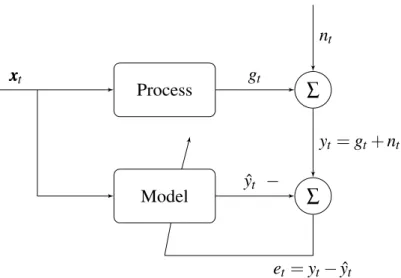
Figure 1 – Example of a system identification problem, where a model is adapted in
order to represent the unknown process behavior. . . 31
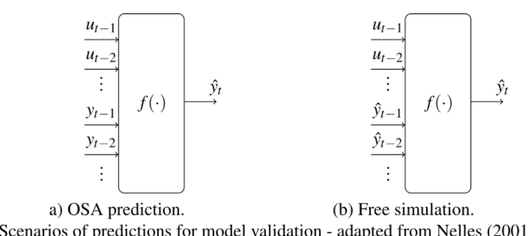
Figure 2 – Scenarios of predictions for model validation - adapted from Nelles (2001). 33 Figure 3 – Example of 2-steps ahead prediction task - adapted from Nelles (2001). . . . 34
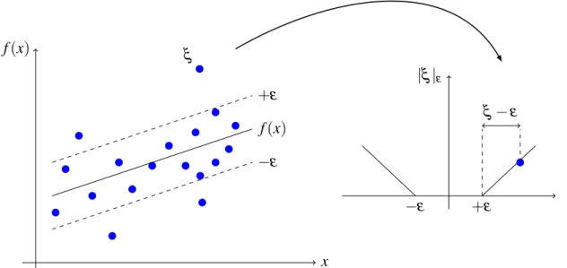
Figure 4 – Illustration of the SVR regression curve with theε-insensitive zone and the slack variables (left); Vapnikε-insensitive loss function (right). . . 44
Figure 5 – Comparison between the standard LSSVR, W-LSSVR and IR-LSSVR models for estimating the sinc function in the presence of outliers. . . 68
Figure 6 – Basic configuration of a linear adaptive filter system. . . 72
Figure 7 – Basic configuration of a kernel adaptive filter system. . . 79
Figure 8 – Probability density functions of the Student’s t and Gaussian distributions. . 102
Figure 9 – Input and output sequences of the Synthetic-1 dataset. . . 103
Figure 10 – Input and output sequences of the Synthetic-2 dataset. . . 103
Figure 11 – Input and output sequences of the Actuator dataset. . . 104
Figure 12 – Input and output sequences of the Dryer dataset. . . 104
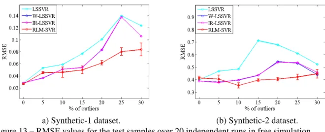
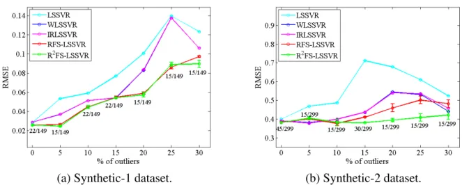
Figure 13 – RMSE values for the test samples over 20 independent runs in free simulation.106 Figure 14 – Predicted outputs by the best models in Table 6 with their worst performances in RMSE over the 20 runs - Actuator dataset. . . 108
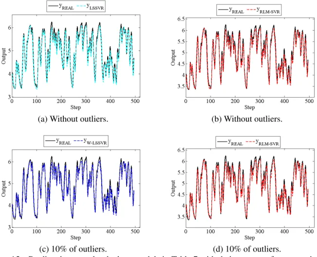
Figure 15 – Predicted outputs by the best models in Table 7 with their worst performances in RMSE over the 20 runs - Dryer dataset. . . 110
Figure 16 – Input and output sequences - Silverbox dataset. . . 119
Figure 17 – Input and output sequences of the Industrial dryer dataset - MIMO system. . 119
Figure 18 – RMSE values for the test samples over 20 independent runs in free simulation.121 Figure 19 – Predicted outputs by the best models in Table 9 with their worst performances in RMSE over the 20 runs - Actuator dataset. . . 123
Figure 20 – Predicted outputs by the best models in Table 10 with their worst perfor-mances in RMSE over the 20 runs - Dryer dataset. . . 125
Figure 21 – Boxplots for the RMSE values of test samples after 20 independent runs -Silverbox dataset. . . 126
Actuator dataset. . . 142
Figure 24 – Predicted outputs by the model with worst performance in RMSE along the 20 runs for the outlier-free scenario - Actuator dataset. . . 144
Figure 25 – Predicted outputs by the model with worst performance in RMSE along the 20 runs for the scenario with 10% of outliers - Actuator dataset. . . 144
Figure 26 – Correlation tests for input-output models - Synthetic-1 dataset with 30% of outliers. . . 146
Figure 27 – Correlation tests for input-output models - Synthetic-2 dataset with 30% of outliers. . . 147
Figure 28 – Correlation tests for input-output models - Actuator dataset with 10% of outliers. . . 148
Figure 29 – Correlation tests for input-output models - Silverbox dataset with 5% of outliers.149 Figure 30 – Convergence curves for the evaluated online models. . . 151
Figure 31 – Obtained RMSE values and predicted outputs for the sinc function. . . 159
Figure 32 – Prediction of the laser time-series with 100 test samples. . . 161
Figure 33 – Prediction of the laser time-series with 500 test samples. . . 161
Figure 34 – Prediction of the laser time-series with 500 test samples for LSSVR and OS-LSSVR models. . . 161
Figure 35 – Obtained RMSE values and predicted outputs for the Synthetic1 dataset -system identification task. . . 163
Figure 36 – Obtained RMSE values and predicted outputs for the Synthetic2 dataset -system identification task. . . 164
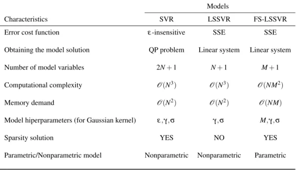
Table 1 – Examples of kernel functions. . . 47 Table 2 – Comparison of some important characteristics of the SVR, LSSVR and
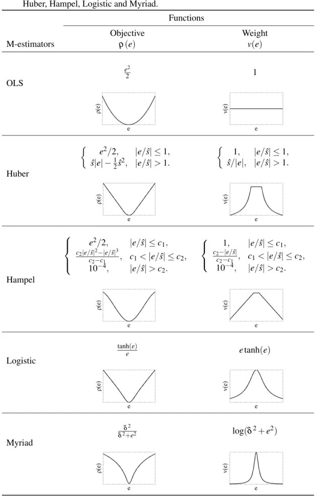
FS-LSSVR models. . . 57 Table 3 – Examples of the objectiveρ(·)and weightv(·)functions for the M-estimators:
OLS, Huber, Hampel, Logistic and Myriad. . . 63 Table 4 – List of kernel adaptive algorithms related to the KAPA family - adapted
from Liu and Príncipe (2008). . . 91 Table 5 – Important features of the evaluated datasets and models for the computational
experiments. . . 104 Table 6 – RMSE for the test samples over 20 independent runs in 3-step-ahead prediction
scenario - Actuator dataset. . . 107 Table 7 – RMSE for the test samples over 20 independent runs in free simulation scenario
- Dryer dataset. . . 109 Table 8 – Important features of the evaluated datasets and models for the computational
experiments. . . 120 Table 9 – RMSE values for the test samples and number of PVs for each evaluated
model - Actuator dataset. . . 123 Table 10 – RMSE values for the test samples and number of PVs for each evaluated
model - Dryer dataset. . . 125 Table 11 – RMSE values for test samples for the Industrial Dryer dataset (MIMO system)
in outlier-free scenario. . . 126 Table 12 – RMSE values for test samples for Industrial Dryer dataset (MIMO system) in
scenario with 5% f outliers. . . 128 Table 13 – Important features of the evaluated datasets and models for the computational
experiments. . . 140 Table 14 – Average number of training input vectors chosen as SVs for the synthetic
datasets. . . 141 Table 15 – RMSE values for test samples and number of SVs for each evaluated model
model - Silverbox dataset. . . 165 Table 18 – AIC and BIC information criteria for all the evaluated models. . . 167 Table 19 – Average norm of the parameter vectorααα for the LSSVR model and ˜αααt for the
Algorithm 1 – - Pseudo-code for the LSSVR model. . . 51
Algorithm 2 – - Pseudo-code for the FS-LSSVR model. . . 56
Algorithm 3 – - Pseudo-code for the IRLS algorithm. . . 62
Algorithm 4 – - Pseudo-code for the W-LSSVR model. . . 66
Algorithm 5 – - Pseudo-code for the IR-LSSVR model. . . 68
Algorithm 6 – - Pseudo-code for the LMS algorithm. . . 75
Algorithm 7 – - Pseudo-code for the RLS algorithm. . . 78
Algorithm 8 – - Pseudo-code for the KLMS algorithm. . . 81
Algorithm 9 – - Pseudo-code for the KRLS model. . . 86
Algorithm 10 – Pseudo-code for the RLM-SVR model. . . 100
Algorithm 11 – - Pseudo-code for the RFS-LSSVR model. . . 113
Algorithm 12 – - Pseudo-code for the R2FS-LSSVR model. . . 114
Algorithm 13 – - Pseudo-code for the ROB-KRLS model. . . 138
AIC Akaike’s Information Criterion ALD Approximate Linear Dependency APA Affine Projection Algorithms BIC Bayesian Information Criterion
FS-LSSVR Fixed Size Least Squares Support Vector Regression i.i.d. Independent and Identically Distributed
IQR Interquatile Range
IRLS Iteratively Reweighted Least Squares
IR-LSSVR Iteratively Reweighted Least Squares Support Vector Regression KAF Kernel Adaptive Filtering
KAPA Kernel Affine Projection Algorithms
KKT Karush-Kuhn-Tucker
KLMS Kernel Least Mean Squares KMC Kernel Maximum Correntropy KRLS Kernel Recursive Least Squares
KRMC Kernel Recursive Maximum Correntropy LMS Least Mean Squares
LS Least Squares
LSSVM Least Squares Support Vector Machine LSSVR Least Squares Support Vector Regression MIMO Multiple-Input Multiple-Output
MSE Mean Squared Error
NARX Nolinear Auto-Regressive with eXogenous input NC Novelty Criterion
OLS Ordinary Least Squares
OSA One-Step Ahead
OS-LSSVR Online Sparse Least Squares Support Vector Regression
PV Prototype Vector
QP Quadratic Programming RFS-LSSVR Robust Fixed Size LSSVR
RLS Recursive Least Squares RLM Recursive Least M-estimate
RLM-SVR Recursive Least M-estimate Support Vector Regression RMSE Root Mean Square Error
ROB-KRLS ROBust Kernel Recursive Least Squares SISO Single-Input Single-Output
SSE Sum of Squared Errors
SV Support Vector
SVM Support Vector Machine SVR Support Vector Regression TSP Time Series Prediction
D Set of input and output training/estimation pairs
Dt Set of input and output training/estimation pairs built up the instantt Dpv Set of prototype vectors (FS-LSSVR)
Dsv
t Dictionary of support vectors built up the instantt (KRLS) mt Cardinality of the dictionary
R Set of the real numbers
N Number of data samples used for training/estimation N′ Number of data samples used for test/validation xxxn n-th input vector
xxxt Input vector built up the instantt
un,ut n-th ort-th control input (system identification task) nt t-th random noise component
d Dimensionality of the input space dh Dimensionality of the feature space yn,yt n-th ort-th real output
yyyt Vector of outputs built up the instantt
ˆ
yn,yˆt n-th ort-th predicted output Lu Memory order of the system input Ly Memory order of the system output
ˆ
Lu Estimate for the memory order of the system input
ˆ
Ly Estimate for the memory order of the system output f(·) Linear/nonlinear regression function
ˆ
f(·) Approximate solution for the function f φφφ(·) Nonlinear map into the feature space
ˆ
φφφ(·) Approximation of the feature mappingφφφ
ˆ
ΦΦΦt Matrix of the projected vectors built up the instantt (KRLS) www Vector of unknown parameters
ˆ
www Approximate solution forwww
ˆ
wwwr Robust solution for ˆwww b Bias of the regression model br Robust solution forb
ˆ
b Approximate solution forb
ˆ
br Robust solution for ˆb en,et n-th ort-th prediction error
vn,vt Weight associated to then-th ort-th prediction error (M-estimators) VVV Diagonal matrix of the weightsvn’s
VVVt Diagonal matrix of the weightsvt’s built up the instantt Jp Functional of an optimization problem in the primal space Jd Functional of an optimization problem in the dual space
L Lagrangian
γ Regularization parameter
αn n-th Lagrange multiplier orn-th coefficient of the solution vector αr
n n-th robust version forαn
αααt Vector of coefficients built up the instantt
˜
αααt Reduced vector ofmt coefficients built up the instantt
˜
αααrt Robust solution for the vector ˜αααt k(·,·) Kernel function
σ Bandwidth of Gaussian kernel function
KKK Kernel (or Gram) matrix
KKKt Kernel matrix built up the instantt
˜
KKKt Kernel matrix built with the dictionary samples up the instantt
¯
HR Quadratic Rényi’s entropy
ρ(·) Objective function or loss function for M-Estimators
ψ(·) Score function for M-estimators ˆ
s Error (outlier) threshold or tunning constant E{·} Statistical expectation operator
(·)† Pseudo-inverse matrix k · k Euclidean norm
p p
pt t-th cross-correlation vector between the output and input signals RRRt t-th input signal correlation matrix
µ Step-size paramater or learning step
λ Forgetting factor
∇∇∇ Gradient vector
ν sparsity level parameter
δt t-th solution of the ALD criterion
1 INTRODUCTION . . . 25 1.1 General and Specific Objectives . . . 29 1.2 The System Identification Problem . . . 30 1.2.1 Classes of Models . . . 31 1.2.2 Model Validation . . . 32 1.2.3 Additional Remarks . . . 35 1.3 Scientific Production . . . 36 1.4 Thesis Structure . . . 38 2 SUPPORT VECTOR REGRESSION MODELS . . . 40 2.1 Introduction . . . 40 2.2 Support Vector Regression - A Brief Discussion . . . 42 2.2.1 SVR for Linear Regression . . . 42 2.2.2 SVR for Nonlinear Regression . . . 45 2.3 Least Squares Support Vector Regression . . . 48 2.3.1 Estimation in the Dual Space . . . 48 2.4 Fixed Size Least Squares Support Vector Regression . . . 51 2.4.1 Estimation in Primal Weight Space . . . 51
2.4.1.1 Approximation to the Feature Map . . . 52 2.4.1.2 Imposing Sparseness and Subset Selection . . . 53 2.4.1.3 The FS-LSSVR Solution . . . 54
2.5 Concluding Remarks . . . 56 3 ROBUSTNESS IN LSSVR DERIVED MODELS . . . 58 3.1 Introduction . . . 58 3.2 Fundamentals of theM-Estimators . . . 60
4.2 Linear Adaptive Filtering . . . 72 4.2.1 Wiener Filter . . . 73 4.2.2 Least Mean Square Algorithm . . . 74 4.2.3 Recursive Least Squares Algorithm . . . 75 4.3 Kernel Adaptive Filtering . . . 78 4.3.1 Kernel LMS Algorithm . . . 79 4.3.2 Kernel RLS Algorithm . . . 80
4.3.2.1 Case 1 - Unchanged Dictionary . . . 83 4.3.2.2 Case 2 - Updating the Dictionary . . . 84
4.4 Other Sparsification Criteria . . . 86 4.5 Other Online Kernel Models. . . 88 4.6 Concluding Remarks . . . 92
5 NOVEL ROBUST KERNEL-BASED MODELS IN BATCH MODE . . 94
5.1 Introduction . . . 94 5.2 Proposed Robust Approach in Dual Space . . . 96 5.2.1 The RLM-SVR Model . . . 97 5.2.2 Computational Experiments . . . 99
5.2.2.1 Evaluated Datasets . . . 101 5.2.2.2 Results and Discussion . . . 103 5.2.2.2.1 Experiments with Synthetic Datasets . . . 105 5.2.2.2.2 Experiments with Real-World Datasets . . . 105
5.3 Proposed Robust Approaches in Primal Space . . . 107 5.3.1 The RFS-LSSVR Model. . . 110 5.3.2 The R2FS-LSSVR Model . . . 112 5.3.3 Extension to Nonlinear MIMO Systems . . . 113
5.3.3.1 The Regression Vector - MIMO Case . . . 116
5.3.4 Final Remarks on the Proposed Models . . . 117 5.3.5 Computational Experiments . . . 117
5.3.5.2.3 Experiments with a Large-Scale Dataset . . . 124 5.3.5.2.4 Experiments with a MIMO Dataset . . . 124
5.4 Concluding Remarks . . . 126 6 NOVEL ONLINE KERNEL-BASED MODELS . . . 130 6.1 Introduction . . . 130 6.2 Proposed Robust KAF Model . . . 132 6.2.1 The ROB-KRLS Model . . . 133
6.2.1.1 Case 1 - Unchanged Dictionary . . . 135 6.2.1.2 Case 2 - Updating the Dictionary . . . 136 6.2.1.3 On the Choice of the Weight Function . . . 137
6.2.2 Computational Experiments . . . 139
6.2.2.1 Results and Discussion . . . 140 6.2.2.1.1 Experiments with Synthetic Datasets . . . 140 6.2.2.1.2 Experiments with Real-World Datasets . . . 143 6.2.2.2 Correlation Analysis of the Residuals . . . 145 6.2.2.3 Convergence Analysis . . . 150
6.3 Proposed Online LSSVR Model . . . 152 6.3.1 The OS-LSSVR Model . . . 153
6.3.1.1 Case 1 - Unchanged Dictionary . . . 155 6.3.1.2 Case 2 - Updating the Dictionary . . . 156
6.3.2 Computational Experiments . . . 159
6.3.2.1 Results and Discussion . . . 160 6.3.2.1.1 Function Approximation . . . 160 6.3.2.1.2 Long-Term Time Series Prediction. . . 162 6.3.2.1.3 Free-Simulation System Identification . . . 164 6.3.2.1.4 Performance on a Large-Scale Dataset . . . 165 6.3.2.2 Convergence Analysis . . . 166 6.3.2.3 Model Efficiency . . . 167 6.3.2.4 A Note on the Norm of the Solution Vector . . . 169
1 INTRODUCTION
“Work gives you meaning and purpose and life is empty without it.” (Stephen Hawking)
Nonlinear phenomena are commonly encountered in most practical problems in areas such as Engineering, Physics, Chemistry, Biology, Economy, etc. This nonlinear nature can be revealed by several sources of non-linearity, including harmonic distortion, chaos, limit cycle, bifurcation and hysteresis (ZHANG; BILLINGS, 2015). Therefore, the data analysis in these cases often requires nonlinear regression methods to detect the kind of dependencies that allow for the successful prediction of properties of interest (HOFMANNet al., 2008).
In this scenario, the kernel-based methods have been proven to be suitable tools to deal with nonlinear regression problems. Inspired by the statistical learning theory (VAPNIK, 1995; VAPNIK, 1998), the Support Vector Regression (SVR) (SMOLA; VAPNIK, 1997) and Least Squares Support Vector Regression (LSSVR) (SUYKENSet al., 2002b; SAUNDERS et al., 1998) non-parametric models, among others, have achieved acceptable performance in
several regression tasks, including function approximation, time series prediction and system identification.
The basic idea behind the kernel methods is that they build a linear model in the so called feature space, where the original pattern inputs are transformed by means of a high-dimensional or even infinite-high-dimensional nonlinear mappingφφφ. Then, the problem is converted from the primal space to the dual space by applying Mercer’s theorem and a positive kernel function (SCHÖLKOPF; SMOLA, 2002), without the need for explicitly computing the mapping
φφφ. This appealing property of the kernel-based methods is referred to as thekernel trick.
It should be noted that the termkernelmay assume different meanings, depending
on the nonlinear modeling paradigm. In Volterra series models (ZHANG; BILLINGS, 2017), for example, the kernel can be regarded as a higher-order impulse response of the dynamic system. In reproducing kernel Hilbert spaces (RKHS)-based techniques, such as the ones followed in the current thesis, the kernelper sedoes not have a signal processing connotation. It is related to
Mercer-type kernels for nonlinear transformation on Machine Learning algorithms, popularized by Vapnik (1998) via the Support Vector Machine (SVM) classifier. In such kernels, there are no memory (i.e. dynamical) issues involved. It is a purely static transformation.
respect to the sparsity of the solution, since in the LSSVR model all the training examples are used as support vectors in order to make new predictions, the learning process in both kernel-based models is carried out inbatch mode. This means that all training samples are stored in
computer memory for building the kernel (Gram) matrix used during the parameter optimization phase. If computer memory cannot hold all of the training data, one can resort to disk storage, but it tends to slow down the learning speed. In addition, if a new data sample is to be added to the model, the kernel matrix computation and the respective parameter optimization process have to be carried out again.
From the 2000s decade, much attention has been focused on developing LSSVR derived methods in order to obtain sparse solutions and, consequently, achieve greater scal-ability in the inherent batch learning. This problem was addressed, for example, by using pruning (SUYKENSet al., 2002a) and fixed-size approaches (SUYKENSet al., 2002b). The
latter, called theFixed-Size LSSVR(FS-LSSVR) model, provides an alternative solution for the
LSSVR formulation in the primal space, which is sparse since it relies on a selected subsample of pattern inputs. The FS-LSSVR model has been widely used to solve static (DE-BRABANTERet al., 2010; MALL; SUYKENS, 2015) and dynamical (DE-BRABANTERet al., 2009a; CASTRO et al., 2014; LEet al., 2011) regression problems.
However, in several specific application domains, such as time series prediction, control systems, system identification and channel equalization, online (i.e. sample-by-sample) learning strategies are required, where the predictor model is modified following the arrival of each new sample. It should be noted that those are classical signal processing applications, but online learning has also gained increasing attention in recent years from the Machine Learning community, due to its inherent ability to handle the demands of big data applications (HOIet al.,
2014; SLAVAKISet al., 2014) and also data nonstationarity (DITZLERet al., 2015).
Strongly motivated by the success of the SVR/LSSVR models in nonlinear regression, the application of the kernelization philosophy to linear adaptive filters has produced powerful nonlinear extensions of well-known signal processing algorithms (ROJO-ÁLVAREZet al., 2014),
including the Least Mean Squares (LMS) (LIUet al., 2008; CHAUDHARY; RAJA, 2015), the
Normalized LMS (SAIDEet al., 2015), and the Recursive Least Squares (RLS) (ENGELet al.,
2004; LIUet al., 2009b; ZHUet al., 2012; SAIDEet al., 2013; FAN; SONG, 2013) algorithms.
In essence, the KAF algorithms are online kernel-based methods that aim to recover a signal of interest by adapting their parameters as new data become available. In this work, the term “online" means that the learning process can be updated one-by-one, without re-training using all the learning data when a new input sample becomes available (LIet al., 2013).
Furthermore, the number of computations required per new sample must not increase (and preferably be small) as the number of samples increases (ENGELet al., 2004).
Of particular interest to this thesis is the work of Engelet al.(2004), who introduced
the Kernel Recursive Least-Squares (KRLS) algorithm as a kernelized version of the famed
RLS algorithm (HAYKIN, 2013; LI et al., 2014), based on an online sparsification method
calledapproximate linear dependence(ALD) (ENGELet al., 2002), that sequentially admits
into a dictionary of kernel representation only those samples that cannot be approximately represented by a linear combination of samples that were previously admitted assupport vectors
(SVs). In summary, the ALD criterion, as well as other sparsification rules, aims at identifying kernel functions whose removal is expected to have negligible effect on the quality of the model solution (RICHARDet al., 2009).
Regarding the discussion above, a common characteristic of the batch LSSVR and FS-LSSVR models, and of the online KRLS algorithm, is that they are built uponsum of squared errors(SSE) cost functions. Then, their optimality is guaranteed only for normally distributed
errors1 and, consequently, the performance of its solution can drastically degrades or even completely breaks down when the evaluated data is corrupted with outlier-like2 samples, e.g. impulsive disturbances (SUYKENSet al., 2002b; SUYKENSet al., 2002a; PAPAGEORGIOU et al., 2015; ZOUBIRet al., 2012).
In this scenario, M-estimation is a broad robust statistics framework (HUBER; RONCHETTI, 2009; ROUSSEEUW; LEROY, 1987) successfully used for parameter estimation in signal processing problems (ZHANGet al., 2014; ZOUBIRet al., 2012), when the Gaussianity
assumption for the prediction errors (i.e. residuals) does not hold. According to this framework, robustness to outliers is achieved by minimizing another function than the sum of the squared errors.
Although M-estimators have been widely used to robustify the standard dual LSSVR
1The least squares estimate is the best linear unbiased estimate of the true parameters of a model if the noise
is white. This means that the covariance matrix of the estimated parameters is the smallest of all possible linear unbiased estimators. If the white noise is also Gaussian, then there does not even exist a better nonlinear unbiased estimator (NELLES, 2001).
2Although there is no universal definition of outlier (HODGE; AUSTIN, 2004), in this thesis we consider an
model (SUYKENSet al., 2002a; DE-BRABANTERet al., 2009b; DEBRUYNE ANDREAS
CHRIST-MANN; SUYKENS, 2010; DE-BRABANTER et al., 2012; DEBRUYNE et al., 2008), the
adopted robust strategies usually modify the original LSSVR loss function applying weighted procedures. In addition, the LSSVR derived models have been little used for robust system identification tasks, and generally only in one-step ahead prediction scenarios (FALCKet al.,
2009; LIU; CHEN, 2013a; LIU; CHEN, 2013b). Regarding the primal LSSVR formulation, the development of robust strategies for the FS-LSSVR model is still an entirely open issue.
As before mentioned, the KRLS model inherits from the RLS algorithm its high sensitivity to outliers. It is then desirable for the KRLS algorithm to be endowed with some inherent mechanism to handle outliers smoothly. One may argue that the simplest approach would be to employ some of the robust strategies used for the linear RLS-based models in the KRLS algorithm. However, such direct transfer is not always straightforward because the resulting KRLS algorithm must satisfy the following three requirements: (i) it must be capable
of handling nonlinearities; (ii) it must be suitable for online learning; and (iii) it must provide a
sparse solution to the parameter vector. Preferably, the sparsification and online learning issues should be unified in the same framework.
Due to these requirements, strategies for building outlier-robust kernel adaptive filtering algorithms are not widely available yet, despite their importance to real-world applica-tions. An important attempt in this direction has been recently introduced by Wuet al.(2015),
who developed a robust kernel adaptive algorithm based on the maximum correntropy criterion (MCC) (LIU; WANG, 2007). MCC is built upon information theoretic concepts and aims at substituting conventional 2nd-order statistical figures of merit, such as Mean Squared Error
(MSE), in order to capture higher-order statistics and offer significant performance improvement, especially when data contain large outliers or are disturbed by impulsive noises.
Despite the rapidly growing number of successful applications of the aforementioned kernel-based online learning models, their use for nonlinear online system identification has not been fully explored yet. This is particularly true for scenarios contaminated with outliers and/or non-Gaussian errors, where just a few works can be found (WUet al., 2015; SANTOSet al.,
2015; LIU; CHEN, 2013b; QUANet al., 2010; TANGet al., 2006; SUYKENSet al., 2002a).
However, most of these previous works (SANTOSet al., 2015; LIU; CHEN, 2013b; QUANet al., 2010; SUYKENSet al., 2002a) cannot be applied to online nonlinear system identification
scheme. In other words, they use all the available training input-output pairs for model building purposes. Sparse solutions, when offered, are achieved via post-training pruning procedures (SUYKENSet al., 2002a).
Finally, an additional difficulty in dealing with (online) system identification prob-lems in the presence of outliers is due to the own dynamic nature of the adopted model. In this case, even considering a possible contamination of outliers only in the output variablesy, their
previously values are used to build the regressor vectors that will be used as input samples for the next time iterations, and so on. Then, the effect of outliers may be felt in both input and outputs of the system. In this scenario, one can conclude that the system identification task becomes even more difficult.
1.1 General and Specific Objectives
In a broader sense, the overall objective in this thesis is to propose novel robust and/or online kernel-based approaches for dynamic system identification tasks in the presence of outliers. Furthermore, one expects that the proposed models, which are derived from the M-estimators theory and kernel adaptive filtering algorithms, achieve suitable performances in terms of generalization capacity when compared to classical methods of the state-of-the-art. In order to accomplish that, we may specifically follow the next steps:
• Propose robust versions (based on the M-estimators) of the LSSVR model in batch learning mode, following its standard dual formulation and the primal space formulation of the FS-LSSVR model;
• Present a novel robust kernel adaptive filtering model, based on the M-estimators and derived from the original KRLS model, for online signal processing in the presence of outliers;
• Propose a sparse and online version of the standard LSSVR model, based on the original KRLS learning procedure;
1.2 The System Identification Problem
The framework of mathematical modeling involves strategies in developing and implementing mathematical models of real systems. According to Billings (2013), a mathe-matical model of a system can be used to emulate this system, predict its outputs for given inputs and investigate different design scenarios. However, these objectives can only be fully achieved if the model of the system is perfectly known. This case corresponds to thewhite-box modeling(SJÖBERGet al., 1995), where it is possible to construct the original model entirely
from prior knowledge and physical insight.
As an alternative to white-box modeling, system identification emerges as an impor-tant area that studies different modeling techniques, where no physical insight is available or used. These techniques are referred to asblack-box modeling, wherein the challenge of describing
the dynamic behavior of the systems consists of searching for a mathematical description from empirical data or measurements in the system (SJÖBERGet al., 1995). Therefore, the black-box
modeling framework corresponds to the focus of this thesis.
System identification is a regression-like problem where the input and output ob-servations come from time series data. In other words, information about the dynamics (i.e. temporal behavior) of the system of interest must be learned from time series data. When nonlinear dynamics has to be captured from data, many modeling paradigms are available in the literature, including neural networks (NARENDRA; PARTHASARATHY, 1990), kernel-based models (ROJO-ÁLVAREZet al., 2004; CAIet al., 2013; GRETTONet al., 2001), fuzzy
systems (TAKAGI; SUGENO, 1985), neuro-fuzzy systems (JANG, 1993), Volterra series repre-sentation (ZHANG; BILLINGS, 2017), Hammerstein-Wiener models (WILLSet al., 2013), and
Chebyshev polynomials approximation (ZHANGet al., 2013), in addition to others.
Mathematically, the representation of a typical nonlinear system identification prob-lem can be expressed, for the sake of simplicity and without loss of generality, by asingle-input single-output(SISO) dynamic system from a finite set of N pairs of observed measurements D ={ut,yt}N
t=1, where ut ∈R is thet-th input and yt ∈R is the output at timet. Then, the
input-output discrete time relationship can be given by
yt=g(xxxt) +nt=gt+nt, (1.1)
where gt ∈R is the true (noiseless) output of the system, g(·) is the unknown, and usually
Process ∑
∑
Model
xxxt gt
nt
yt=gt+nt
ˆ
yt −
et=yt−yˆt
Figure 1 – Example of a system identification problem, where a model is adapted in order to represent the unknown process behavior.
independent and identically distributed (i.i.d.) with zero mean and finite variance. xxxt denotes the regression vector at sampling timet and its components are given as a function of the relevant
variables of the system at a previous time.
An example of a system identification problem for a SISO system is illustrated in Fig. (1), where the model predictions should represent the dynamical behavior of the process as closely as possible. The model performance is typically evaluated in terms of a function of the erroret between the noisy process outputyt and the model output ˆyt. Then, this error is used to
adjust the parameters of the model.
1.2.1 Classes of Models
In order to construct or select models in system identification scenarios, the first step is determining a class of models within which the search for the most suitable model is to be conducted. For this purpose, a number of different linear models have been proposed (LJUNG, 1999; BILLINGS, 2013; AGUIRRE, 2007), such as Auto-Regressive (AR), Auto-Regressive with eXogenous inputs (ARX), Moving Average (MA), Auto-Regressive Moving Average (ARMA), Auto-Regressive Moving Average with eXougenous inputs (ARMAX), Output Error (OE), Finite Impulse Response (FIR) and Box-Jenkis (BJ). One should note that the respective nonlinear versions follow a similar nomenclature of these linear models.
Among the nonlinear dynamic models, theNonlinear Auto-Regressive with eXoge-nous inputs(NARX) covers a wide class of nonlinear systems and it is normally the standard
the major goal in this thesis is not to find the best model for a given application, but rather, evaluate the performance of parameter estimation techniques for kernel-based models, the NARX dynamic model will be used for all the applications in system identification throughout this work. The NARX model can be defined by rewriting Eq. (1.1) as (BILLINGS, 2013; AGUIRRE, 2007; NELLES, 2001)
yt=g(yt−1, . . . ,yt−Ly,ut−τd, . . . ,ut−Lu) +nt, (1.2) whose regression vector is given by
xxxt= [yt−1, . . . ,yt−Ly,ut−τd, . . . ,ut−Lu]⊤, (1.3)
where it is assumed that the random noisent in Eq. (1.2) is i.i.d. and is purely additive to the
model. TheLu≥1 andLy≥1 values are the maximum lags for the system input and output,
respectively, denoting their memory orders. The target nonlinear functiong(·):RLy+Lu→Ris assumed to be unknown andτdis a time delay, also called dead time, typically set toτd=1.
In the next step, the observed data in the form of input-output time series should be used to build an approximating model f(·)for the target functiong(·), which is expressed by
ˆ
yt= f(yt−1, . . . ,yt−Lˆy,ut−1, . . . ,ut−Lˆu), (1.4) where ˆLu and ˆLy are estimates of the real system memory. Clearly, the regressors xxxt, and
consequently the model f(·), depend on ˆLuand ˆLy, but these dependencies have been omitted in
order to simplify the notation, as was done by SOUZA-JÚNIOR (2014).
The techniques for developing nonlinear mappings f(·) strategies, derived from kernel-based models, and their required procedures for parameter estimation are the main purpose of this thesis and, therefore, they will be discussed in detail throughout next chapters.
1.2.2 Model Validation
f(·)
ut−1
ut−2 ...
yt−1
yt−2 ...
ˆ
yt
f(·)
ut−1
ut−2 ... ˆ
yt−1 ˆ
yt−2 ...
ˆ
yt
a) OSA prediction. (b) Free simulation.
Figure 2 – Scenarios of predictions for model validation - adapted from Nelles (2001).
model serves to explain another observed dataset of the same system (AGUIRRE, 2007). This strategy is used to measure the generalization capacity of the model.
Since the model was properly obtained, it may be used to simulate the dynamical output of the identified system through iterative predictions. In this sense, there are two possible scenarios: predictionand simulation. Prediction means that, on the basis of previous inputs ut−i (for i=1, . . . ,Lˆu) and outputs yt−j (for j=1, . . . ,Lˆy), the model predicts one or several
steps into the future, while simulation means that the model simulates future outputs only on the basis of previous inputsut−i(NELLES, 2001). Simply stated, prediction uses previous values
of inputs and observed outputs to predict the current output, whereas simulation uses previous values of inputs and predictions (rather than observed outputs) to predict the current output.
The simplest concept in prediction scenarios is that of One-Step Ahead (OSA)
prediction, in which the vector of regressors xxxt−1 at time instantt−1 is first built, based on previous values of observed outputs and inputs, only to compute the predicted output ˆyt for the
next time instantt. However, it is noteworthy that this prediction ˆyt is not used to obtain the next
OSA prediction ˆyt+1. The output given by Eq. (1.4) is considered as a OSA prediction, because ˆ
yt is computed from measured outputs up to time instantt−1. Fig. (2a) illustrates the task of
one-step ahead prediction.
f(·)
ut−2
ut−3
yt−2
yt−3
f(·)
ut−1
ut−2
yt−2 ˆ
yt−1
ˆ
yt
Figure 3 – Example of 2-steps ahead prediction task - adapted from Nelles (2001).
the test samples can be almost perfect. Therefore, it can be concluded that OSA predictions are not appropriate to explain the dynamic behavior of the identified system.
In contrast to OSA, in simulation scenarios the previous predictions are used to build the vector of regressors in order to continue making predictions. Thus, the vector of regressors is expressed as
xxxt= [yˆt−1, . . . ,yˆt−Lˆy,ut−1, . . . ,ut−Lˆu]
⊤, (1.5)
where the process inputsut−i, fori=1, . . . ,Lˆu, are always available, as in the case of OSA. The
output simulated according to Eq. (1.5) is calledfree simulationorinfinite-steps ahead prediction,
and it is illustrated in Fig. (2b).
Free simulation tasks are often required for applications in optimization, control, system identification and fault detection, where in some circumstances it becomes difficult (or even impossible) to measure the process outputs. In free simulation, as may be inferred, predictions rely on previous predictions and, consequently, the prediction errors tend to propagate through nonlinear transformations. This makes the modeling and identification phase harder, and requires additional care in order to ensure the stability of the model (NELLES, 2001). Even in this hostile scenario, free simulation is, unlike the OSA predictions, a suitable way to test if the model can explain the measured observations (AGUIRRE, 2007).
Regarding the discussion above, one can say that the prediction scenarios of OSA and free simulation are two extreme cases. Nevertheless, there is an intermediate case when more than one step is to be predicted into the future. This case is called themultiple-steps ahead
ork-steps ahead prediction, which consists of using the obtained model as a free predictor only
for ksampling intervals, restarting it immediately afterward with measured data (AGUIRRE,
2007). The number of steps predicted into the futurekdenotes theprediction horizon.
This procedure can be repeatedktimes in order to predictksteps ahead altogether. Then, for k=2,3, . . ., thek-step prediction is recursively computed by (ZHANG; LJUNG, 2007)
ˆ
yt(k)= f(yˆ(t−k−11), . . . ,yˆ(k−1)
t−Lˆy ,ut−1, . . . ,ut−Lˆu), (1.6)
where ˆyt(1),ytˆ, as defined by Eq. (1.4). One should note that the sequence ˆyt(1)(fort=1, . . . ,N′),
whereN′denotes the number of test samples used for model validation, must be first computed
before ˆy(t2)be computed. Then, ˆyt(3) is computed, and so on. Therefore, the predicted output ˆy(tk),
computed with the recurrent expression in Eq. (1.6), can be viewed as ak-steps ahead prediction
ofyt. This scenario is illustrated in Fig. (3) fork=2.
Among the prediction scenarios, it is worth mentioning thatk-steps ahead prediction
task is equivalent to free simulation when the prediction horizon approaches infinity (k→+∞). In this thesis, we do not apply OSA predictions for model validation. For this purpose, we only usek-steps ahead prediction and, in most applications, free simulation.
Finally, a common and useful choice in the quantification of predictions is theRoot Mean Squared Error(RMSE), calculated between the predicted outputs and the real observations
over the whole test dataset. Mathematically, the RMSE value is given by
RMSE=
v u u t 1
N′ N′
∑
t=1(yt−yˆt)2. (1.7)
In principle, the smaller the RMSE value, the better the reconstruction of the system dynamics. Next, some additional remarks are presented in order to clarify and facilitate the understanding about the system identification problems treated throughout this thesis. For more details in the framework of system identification, the reference text-books by Billings (2013), Ljung (1999), Aguirre (2007), Nelles (2001) and Söderström and Stoica (1989) are recommended.
1.2.3 Additional Remarks
Otherwise, the obtained model will not be able to produce reliable predictions of this system.
Regarding the sampling time, a value that is too small (oversampling) causes successive data samples to be very similar, so that the data become redundant. If a sampling time that is too large (undersampling) is chosen, then successive data points tend to become independent from each other so that the dynamical information about the original system is lost (ZHANGet al., 2013).
In this thesis, we abstract away from these particular issues because we use benchmarking datasets for the computational experiments. In this case, we assume that the available estimation datasets are sufficiently representative of the system of interest and, besides that, the sampling rate is suitably chosen and normalized, so that we can treat the systems of interest as intrinsically nonlinear discrete-time systems.
Remark 2 - Several nomenclatures commonly used in system identification and control theories have synonyms somewhat different in the field of Machine Learning. Therefore, in order to avoid confusion with some of them, we provide a glossary of terms (as done in Sjöberget al.(1995), SOUZA-JÚNIOR (2014)) that are used interchangeably with their equivalents
in this thesis:
• estimate = train, learn, model building, structure selection; • validate = test, generalize;
• estimation dataset = training dataset, model building dataset; • validation dataset = test dataset, generalization dataset.
1.3 Scientific Production
Throughout the development of this work, a reasonable number of articles have been published by the author and respective co-authors. Among them, the published articles related to the thesis are:
1. José Daniel A. Santos and Guilherme A. Barreto, Novel Sparse LSSVR Models in Primal Weight Space for Robust System Identification with Outliers. Journal of Process Control, to appear (http://doi.org/10.1016/j.jprocont.2017.04.001), 2017.
2. José Daniel A. Santos and Guilherme A. Barreto,A Regularized Estimation Framework for Online Sparse LSSVR Models. Neurocomputing, vol. 238, 114-125, 2017.
Al-gorithm for Nonlinear System Identification. Nonlinear Dynamics, vol. 90, issue 3,
1707-1726, 2017.
4. José Daniel A. Santos and Guilherme A. Barreto,A Novel Recursive Solution to LS-SVR for Robust Identification of Dynamical Systems. In Lecture Notes in Computer Science: Intelligent Data Engineering and Automated Learning - IDEAL 2015, K. Jackowski, R.
Burduk, K. Walkowiak, M. Wozniak and H. Yin Eds., vol. 9375, 191-198, 2015.
5. José Daniel A. Santos, César Lincoln C. Mattos and Guilherme A. Barreto,Performance Evaluation of Least Squares SVR in Robust Dynamical System Identification. In Lecture Notes in Computer Science: International Work Conference on Artificial Neural
Networks - IWANN 2015, I. Rojas, G. Joya and A. Catala Eds., vol. 9095, 422-435, 2015.
Furthermore, the following published articles were produced during the thesis period as result of research collaborations:
1. César Lincoln C. Mattos, José Daniel A. Santos and Guilherme A. Barreto,An Empirical Evaluation of Robust Gaussian Process Models for System Identification. In Lecture Notes in Computer Science: Intelligent Data Engineering and Automated Learning
-IDEAL 2015, K. Jackowski, R. Burduk, K. Walkowiak, M. Wozniak and H. Yin Eds., vol.
9375, 172-180, 2015.
2. José Daniel A. Santos and Guilherme A. Barreto,Uma Nova Solução Recursiva para LS-SVR em Identificação Robusta de Sistemas Dinâmicos. In:XII Simpósio Brasileiro de
Automação Inteligente (SBAI 2015), Natal (Brazil), 25-28 October 2015, p. 642-647. 3. César Lincoln C. Mattos, José Daniel A. Santos and Guilherme A. Barreto,Uma
Avali-ação Empírica de Modelos de Processos Gaussianos para IdentificAvali-ação Robusta de Sistemas Dinâmicos. In:XII Simpósio Brasileiro de Automação Inteligente (SBAI 2015),
Natal (Brazil), 25-28 October 2015, p. 712-717.
4. José Daniel A. Santos, César Lincoln C. Mattos and Guilherme A. Barreto,A Novel Re-cursive Kernel-Based Algorithm for Robust Pattern Classification. In Lecture Notes in Computer Science: Intelligent Data Engineering and Automated Learning - IDEAL
2014, E. Corchado, J. A. Lozano, H. Quintián and H. Yin Eds., vol. 8669, 150-157, 2014.
5. César Lincoln C. Mattos, José Daniel A. Santos and Guilherme A. Barreto, Improved Adaline Networks for Robust Pattern Classification. In Lecture Notes in Computer Sci-ence: International Conference on Artificial Neural Networks - ICANN 2014, S. Wermter,
579-586, 2014.
6. Davi N. Coelho, Guilherme A. Barreto, Cláudio M. S. Medeiros and José Daniel A. Santos, Performance Comparison of Classifiers in the Detection of Short Circuit Incipient Fault in a Three-Phase Induction Motor. In: IEEE Symposium on Computational
Intelligence for Engineering Solutions (IEEE-CIES 2014), Orlando (EUA), 9-12 December 2014, vol. 01, p. 42-48.
7. César Lincoln C. Mattos, José Daniel A. Santos and Guilherme A. Barreto,Classificação de Padrões Robusta com Redes Adaline Modificadas. In: Encontro Nacional de
In-teligência Artificial e Computacional (ENIAC 2014), São Carlos (Brazil), 19-23 October 2014.
8. Edmilson Q. Santos Filho, José Daniel A. Santos and Guilherme A. Barreto, Estudo Comparativo de Métodos de Extração de Características para Classificação da Qual-idade de Peles de Caprinos com Opção de Rejeição. In: XI Simpósio Brasileiro de
Automação Inteligente (SBAI 2013), Fortaleza (Brazil), 13-17 October 2013, p. 01-06.
1.4 Thesis Structure
The remainder of this thesis is organized as follows.
Chapter 2 presents a brief framework of the kernel-based methods, more specifically, the support vector theory applied to nonlinear regression problems. Besides containing the basic ideas of the SVR model, it discusses in more detail the theoretical development of the LSSVR model in its standard dual formulation and in the primal space, which is referred to as the FS-LSSVR model. Finally, a comparative framework, with the main features of each evaluated kernel-based model: SVR, LSSVR and FS-LSSVR, is presented.
Chapter 3 is dedicated to outlier robustness. It discusses the theoretical foundation of M-estimators, which are presented as an alternative to least squares methods for linear regression problems. Next, some strategies in splice M-estimators to standard LSSVR formulation, giving rise its robust versions W-LSSVR and IR-LSSVR models, are discussed. Moreover, a compu-tational experiment of outliers influence using the above LSSVR derived models is presented. Finally, a brief state-of-the-art about some robust LSSVR approaches is described.
respective kernelized versions KLMS and KRLS are discussed in the sequence. Afterwards, a description of the family of kernel affine projection algorithms (KAPA) and some other sparsification criteria, different from ALD of the KRLS model, are presented.
Chapter 5 introduces the first part of the proposed approaches of this thesis, namely the RLM-SVR, RFS-LSSVR and R2FS-LSSVR models, which correspond to robust kernel-based methods derived from the LS-SVR and FS-LSSVR standard models and based on M-estimators. This chapter also reports the performance results of the novel proposals in several system identification tasks using synthetic, real-world, large-scale and MIMO datasets in the presence of outliers.
Chapter 6 presents the second part of the contributions of this thesis, which comprises two novel kernel adaptive filtering methods derived from the original KRLS model. The first proposal is called ROB-KRLS and corresponds to a robust version of the KRLS model based on M-estimators. The second one, called the OS-LSSVR model, is based on the standard LSSVR formulation and is solved according to the KRLS learning procedure. This chapters also encompasses the results of computational experiments with the proposed approaches in several regression/system identification tasks using synthetic, real-world and large-scale datasets.
Chapter 7 is dedicated to the conclusions of this work as well to the directions for future research on issues related to the thesis.
Appendix A provides a step-by-step mathematical formulation for the ROB-KRLS proposed approach.
Appendix B provides a step-by-step mathematical formulation for the OS-LSSVR proposed approach.
2 SUPPORT VECTOR REGRESSION MODELS
“Things don’t have to change the world to be important.” (Steve Jobs)
This chapter covers the kernel-based models theory, with an emphasis on support vector machines, when applied in nonlinear regression problems. Initially, Section 2.1 makes some considerations on the topics that are treated throughout the chapter. Then, Section 2.2 briefly discusses the basic ideas of Support Vector Regression (SVR), which was the pioneer among the kernel-based methods. Next, the theoretical foundations of the Least Squares Support Vector Regression (LSSVR) (Section 2.3) and Fixed Size Least Squares Support Vector Regression (FS-LSSVR) (Section 2.4) models are developed in detail, since they directly provide the backgrounds for some contributions of this thesis. Finally, Section 2.5 presents the final remarks of the chapter.
2.1 Introduction
The Support Vector Machines (SVM) framework comprises a powerful class of learning algorithms, derived from the results of the statistical learning theory (VAPNIK, 1995). Its development was first presented as a nonlinear generalization of theGeneralized Portrait
algorithm (VAPNIK, 1963; VAPNIK; CHERVONENKIS, 1964) to solve pattern recognition problems (VAPNIK; CHERVONENKIS, 1974; BOSERet al., 1992). Later, it was extended
by Smola and Vapnik (1997) to the domain of regression problems, which will be referred to asSupport Vector Regression(SVR) from now on.
The SVR model works with a constrained quadratic optimization problem, which minimizes a combination of the empirical risk (employed by the conventional neural networks, e.g.) and a regularization term responsible for the smoothness of the model solution. This solution is obtained by solving a convexquadratic programming(QP) problem in dual space
and, thus, has the noteworthy advantage of being a global and sparse solution. By sparseness, one means that the final regressor can be written as a combination of a relatively small number of training patterns, called thesupport vectors(SVs). Therefore, the SVR intrinsic characteristics,
resulting from its strong conceptual formulation, have made it achieve satisfactory performance in a wide variety of regression problems (BAOet al., 2014; KARTHIKet al., 2016; KAZEMet al., 2013; CHEN; YU, 2014).
empirically shown to be not maximally sparse (BURGES; SCHÖLKOPF, 1997; DOWNS et al., 2001). In addition, an SVR optimization problem involves twice as many variables as the
number of training samples and, moreover, the methods to solve the QP problem do not have a trivial implementation. In general, these methods present a super-linear dependence on the computation time of the number of available patterns and require repeated access to the training samples, making them suitable only for batch learning (ENGELet al., 2002).
In this context, theLeast Squares Support Vector Regression(LSSVR) model
(SAUN-DERSet al., 1998; SUYKENSet al., 2002b) was proposed as a simpler alternative method to
the standard Vapnik’s SVR model, since learning in LSSVR relies on an SSE cost function and a set of equality constraints, instead of the original QP problem in SVR. Consequently, the model solution in LSSVR problem is easier to obtain by solving a set of linear equations in its dual formulation. In addition, the LSSVR model inherits from the SVR technique the convexity of the optimization problem and the global solution. On the other hand, the sparsity common to the SVR model is lost in the LSSVR problem, since every training sample contributes to the model solution as an SV.
At present, the LSSVR model has been widely applied to regression tasks, such as time series forecasting (ORMÁNDI, 2008; GESTELet al., 2001; MELLITet al., 2013; CHEN;
LEE, 2015), control (SUYKENSet al., 2001; KHALIL; EL-BARDINI, 2011; ZHANGet al.,
2014) and dynamical system identification (FALCKet al., 2012; LAURAINet al., 2015; CAIet al., 2013).
A key property behind the SVR and LSSVR models is that they apply kernel functions, which only require the evaluation of inner products between pairs of pattern inputs. Replacing inner products with a Mercer kernel provides an efficient way to implicitly map the data into a high, even infinite, dimensional RKHS (SCHÖLKOPF; SMOLA, 2002) by means of a nonlinear feature mapφφφ. Then, the calculations are carried out without making direct reference to the mapping of the input vectors, a property referred to as the kernel trick.
Although the LSSVR model is mostly solved in the dual formulation through the kernel trick, its optimization problem can also be solved in the primal space by estimating the feature mapφφφ. This attempt was introduced by Suykenset al.(2002b), resulting in a parametric
and sparse representation called theFixed-Size Least Squares Support Vector Regression
In the FS-LSSVR model, it is possible to compute sparse and approximated model solution by using only a subset of selected support vectors, also calledprototype vectors(PVs),
from the entire training data. One distinct advantage of this approach is that it can easily handle nonlinear estimation problems that require large amounts of data. Successful applications of the FS-LSSVR model can be found in De-Brabanter et al. (2009a), Espinoza et al. (2006),
De-Brabanteret al.(2010) and Castroet al.(2014).
Finally, one should consider that the LSSVR and FS-LSSVR models serve as basis for some contributions of this thesis. Therefore, they are treated in detail throughout this chapter. On the other hand, the SVR theory is presented as a brief discussion, because of its importance in the development of the area of support vector methods and also for a better understanding in developing the LSSVR and FS-LSSVR models.
2.2 Support Vector Regression - A Brief Discussion
This section presents a brief discussion on linear and nonlinear SVR model, in which the origins of the derivation of the LSSVR formulation will be highlighted. Further details on SVR theory can also be found in Smola and Schölkopf (2004), Basaket al.(2007), Schölkopf
and Smola (2002), Bishop (2006), Cherkassky and Mulier (2007) and Vapniket al.(1996).
2.2.1 SVR for Linear Regression
Consider an estimation/training dataset D ={(xxx1,y1), . . . ,(xxxN,yN)}formed by N
pairs of inputs xxxn∈Rd and corresponding outputsyn∈R, for n=1, . . . ,N. In a regression
problem, the goal is to search for a function f(·)that approximates the outputsynfor all instances
of the available data. Initially, for the linear case, f(·)usually takes the form
f(xxxn) =www⊤xxxnnn+b, (2.1)
wherewww∈Rd is a parameter vector andb∈Ris a bias term. In order to seek flatness in Eq. (2.1), minimizing the Euclidean normk · k2, or simply k · k, ofwwwis required (SMOLA, 1998;
SCHÖLKOPF; SMOLA, 2002). Then, the optimal parameters of the linear function f(·)are searched by minimization of the following constrained functional:
min
www,bJp(www) =
1 2kwwwk
subject to
yn−www⊤xxxn−b≤ε, forn=1, . . . ,N, w
ww⊤xxxn+b−yn≤ε, forn=1, . . . ,N.
(2.3)
The convex optimization problem in Eq. (2.2) with the inequality constraints in Eq. (2.3) is feasible in cases where the function f(·)exists and has, at most,ε deviation from all the training outputs yn and, at the same time, is as smooth as possible. However, sometimes errors are
allowed in introducing slack variables, which describe the penalty for the training patterns lying outside theε boundary. Therefore, the formulation in Eqs. (2.2), (2.3) becomes
min
www,b,ξξξ,ξξξ∗
Jp(www,ξξξ,ξξξ∗) =
1 2kwwwk
2+γ
∑
Nn=1
(ξn+ξn∗), (2.4)
subject to
yn−www⊤xxxn−b≤ε+ξn, w
ww⊤xxxn+b−yn≤ε+ξn∗, ξn,ξn∗≥0,
(2.5)
for n=1, . . . ,N. The values ofξn andξn∗ are slack variables corresponding to the points for
which f(xxxn)−yn>ε (points above the curve) and yn− f(xxxn)>ε (points below the curve),
respectively. The constant γ >0 is a regularization parameter that establishes a trade-off between the smoothness of f(·) and the amount up to which deviations larger than ε are tolerated. This corresponds to dealing with a so calledε-insensitive loss function, or Vapnik loss function (VAPNIK, 1995), described by
|ξ|ε :=
0, if|ξ|<ε
|ξ| −ε, otherwise,
(2.6)
and illustrated on the right side of Fig. (4). One should note that only the points outside the
ε-insensitive zone contribute to the cost function, as can be seen in the blue point close to the symbolξ, on the left size of Fig. (4) .
The parametric formulation in Eq. (2.4) with the inequality constraints in Eq. (2.5) is an optimization problem in the primal weight space, also referred to as a theprimal problem, since
it is defined in the original spaceRd of the input dataxxxnand the parameter vectorwww. The solution
x f(x)
f(x) −ε
+ε ξ
|ξ|ε
+ε
−ε
ξ−ε
Figure 4 – Illustration of the SVR regression curve with the ε-insensitive zone and the slack variables (left); Vapnikε-insensitive loss function (right).
from Eqs. (2.4) and (2.5), as follows:
L(www,b,ξξξ,ξξξ∗;ααα,ααα∗,ζζζ,ζζζ∗) := 1
2kwwwk2+γ
N
∑
n=1(ξn+ξn∗)− N
∑
n=1αn(www⊤xxxn+b−yn+ε+ξn)
−
N
∑
n=1αn∗(yn−www⊤xxxn−b+ε+ξn∗)− N
∑
n=1(ζnξn+ζn∗ξn∗), (2.7)
whereαn≥0,αn∗≥0,ζn≥0,ζn∗≥0 are the Lagrange multipliers andL denotes the Lagrangian,
whose saddle point is characterized by max
(ααα,ααα∗,ζζζ,ζζζ∗≥0)(www,minb,ξξξ,ξξξ∗)L(www,b,ξξξ,ξξξ
∗;ααα,ααα∗,ζζζ,ζζζ∗), (2.8)
where the gradients related to the primal variables are set to zero, according to Karush-Kuhn-Tucker (KKT) conditions for optimality (KARUSH, 1939; KUHN; TUCKER, 1951), such as:
∂L
∂www =000⇒www=∑ N
n=1(αn−αn∗)xxxn,
∂L
∂b =0⇒∑ N
n=1(αn−αn∗) =0,
∂L
∂ ξn =0⇒γ−αn−ζn=0,
∂L
∂ ξn∗ =0⇒γ−αn∗−ζn∗=0.
Using the results of Eqs. (2.9) to eliminate the corresponding variables from the Lagrangian, a new optimization problem can be formulated by the maximization of
max α α
α,ααα∗Jd(ααα,ααα
∗) =−1 2
N
∑
n=1N
∑
m=1(αn−αn∗)(αm−αm∗)xxx⊤nxxxm−ε N
∑
n=1(αn+αn∗) + N
∑
n=1(αn−αn∗)yn,
(2.10) subject to
∑Nn=1(αn−αn∗) =0,
0≤αn≤γ,
0≤αn∗≤γ,
(2.11)
for n=1, . . . ,N. The problem in Eqs. (2.10) and (2.11) corresponds to the formulation of a quadratic programming(QP) problem in the dual weight space, and can also be referred to as
thedual problem. The term “dual" is used because now the problem is solved in the space of 2N
dual variablesαnandαn∗, instead ofwwwin the primal space. Using Eq. (2.1) and the expression
forwwwin Eq. (2.9), the SVR model solution is given by
f(xxx∗) =
N
∑
n=1(αn−αn∗)xxx⊤nxxx∗+b. (2.12)
An important property of the QP problem in Eqs. (2.10), (2.11) is that many resulting values ofαn,αn∗ are equal to zero. Hence, the obtained solution is sparse, i.e. the sum in Eq.
(2.12) should be taken only over non-zero values of(αn−αn∗), instead of all training patterns.
The input examples xxxn, for which the corresponding Lagrange multipliers are not null, are
the support vectors. In addition, note that, unlike the primal space solution in Eq. (2.1), the expressions in Eqs. (2.10)-(2.12) are independent of the parameter vector www. Therefore, one
should say that the SVR dual problem corresponds to a non-parametric model, although its original formulation in Eqs. (2.4) and (2.5) corresponds to a parametric model.
2.2.2 SVR for Nonlinear Regression
The majority of regression problems in machine learning are essentially nonlinear. Therefore, the linear formulation of the SVR model in Section 2.2.1 should be extended to the nonlinear case. Then, given the estimation datasetD ={xxxn,yn}N
n=1, withxxxn∈Rd andyn∈R, the function f(·)in Eq. (2.1) now takes the form