J. G. Janzen
L. B. S. de Souza and
H. E. Schulz
Department of Hydraulics and Sanitation São Carlos School of Engineering – USP Av. do Trabalhador Sancarlense, 400 13560-970 São Carlos, SP. Brazil [email protected], [email protected] and [email protected]Kinetic Energy in Grid Turbulence:
Comparison between Data and Theory
The properties of turbulence induced in a viscous fluid by oscillating a grid within it are investigated. Vertical and horizontal components of fluctuating velocities are measured using the Digital Particle Image Velocimetry technique (DPIV). Vertical profiles of turbulent kinetic energy k, obtained from the fluctuating velocities, are presented and compared with theoretical predictions obtained using the k-ε turbulence model.Keywords: Oscillating grid turbulence, turbulent energy, k-ε model
Introduction
Oscillating grids are often used to generate controlled turbulent fields in viscous fluids, thereby allowing a better understanding of the effect of turbulence on several physical phenomena. Examples are the mixing processes in a stratified fluid (Rouse, 1955; Thompson and Turner, 1975), gas transfer processes at the gas/water interface (Brumley and Jirka, 1987; Chu and Jirka, 1991), sediment suspension (Brunk et al., 1996; Medina et al., 2001), and turbulent
coagulation (Shy et al., 1996), among others.1
A grid (usually square) with mesh sizeM (cm) oscillates around
a mean position with an amplitudeS (the stroke, cm) at a frequency
f (Hz) in a tank filled with a viscous fluid. The turbulence in the
bulk of the tank is the result of the interaction between jets and wakes produced by the movement of the grid. The mean velocity of the flow is zero and turbulence decays with increasing distance from the grid. Literature shows that beyond a distance ranging from one to three mesh sizes from the grid, the turbulence is homogeneous on planes parallel to the grid, with a ratio of vertical to horizontal turbulent intensities in the range of 1.1-1.2 (De Silva and Fernando, 1994).
A number of oscillating-grid experiments have been carried out to study characteristics of turbulence in a homogeneous fluid.
Thompson and Turner (1975) found that the horizontal rms
turbulent velocity (u) is proportional to f and decays with z-1,5.
Hopfinger and Toly (1976) proposed the following empirical equation:
1 5 , 0 5 ,
1 −
=CfS M z
u (1)
For the experimental conditions of Hopfinger and Toly (1976),
the constant C assumed the value 0.25. However, Nokes (1988)
stated that the decay ofu could not be expressed by a simple power
law. Other authors (Schulz and Chaudhry, 1998; Matsunaga et al., 1999) obtained theoretical predictions for the turbulent kinetic
energy k and its dissipation rate ε for oscillating grid turbulence
using thek-ε model. Equation (1) may be considered a special case
of these more refined predictions.
The purpose of the present paper is to report on experimentally
obtained vertical profiles of the turbulent energyk, and to compare
it with theoretical predictions of the k-ε turbulence model.
Paper accepted October, 2003. Technical Editor: Atila P. Silva Freire.
Nomenclature
A = model constant (Schulz and Chaudhry), m4/s2
B = model constant (Schulz and Chaudhry), m C = experimental constant, dimensionless
C2 = k-ε model constant, dimensionless
Cµ = k-ε model constant, dimensionless
f = grid frequency, Hz
h = normalized turbulent energy, dimensionless
k = turbulent energy, m2/s2
k0 = constant used to non-dimensionalize the turbulent energy,
m2/s2
M = grid mesh size, m r = constant, dimensionless
Re = Reynolds number, dimensionless s = nondimensional distance, dimensionless S = grid stroke, m
u = horizontal rms turbulent velocity, m/s u’ = horizontal turbulent velocity, m/s w’ = vertical turbulent velocity, m/s z = vertical coordinate axis, m
z0 = constant used to non-dimensionalizez, m
Greek Symbols
α = model constant (Schulz and Chaudhry), dimensionless
β = model constant (Schulz and Chaudhry), dimensionless
ε = dissipation rate, m2/s3
ε0 = constant used to non-dimensionalize the dissipation rate,
m2/s3
ν = kinematic viscosity, m2/s
νt = eddy viscosity, m2/s
σε = k-ε model constant, dimensionless
σk = k-ε model constant, dimensionless
Subscripts
0 = relative to origin
k = relative to kinetic turbulence energy
µ = relative to viscosity
t = relative to turbulence
Oscillating Grid System
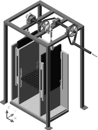
Figure 1 is a schematic representation of the turbulence-generating system used in this study. The experiments were
conducted in a tank built of acrylic plates, with a 0.50 mx 0.50 m
field. A grid was built with 1.0x 1.0 cm square bars in a 5.1 cm mesh size, which resulted in a solidity of 32%. This grid design fulfills the condition proposed by Corrsin (1963), who stated that stable jets and wakes can be obtained only with a solidity less than 40% (see De Silva and Fernando, 1992). To permit easy manipulation of the grid in the tank, a gap of 0.2-0.3 cm was maintained between the sidewalls and the grid. The frequency of the
grid oscillationsf was varied over a range of 1 <f < 4 Hz with a
strokeS of 3 cm. Because the oscillating grid turbulence is sensitive
to the initial conditions, data acquisition began only after 10 min of the onset of oscillation.
Figure 1. Diagram of the oscillating-grid tank. Interior dimensions: area of 2500 cm2 and height of 115 cm.
DPIV
The velocity field is measured by the well-established DPIV (Digital Particle Image Velocimetry) technique (Cheng et al., 1997; Quénot et al., 1998; Cheng and Law, 2001). DPIV is an optical imaging technique which provides instantaneous velocity vector measurements in a plane of a flow. The typical DPIV evaluation procedure is based on the analysis of two sucessive images of the flow. The digital images are decomposed into small subsections called interrogation areas. The content of corresponding interrogation areas of two successive images is cross-correlated to determine the average spatial shift of particle images. The ratio between displacement of particles and the time elapsed between two images gives the average velocity in the interrogation area. A velocity vector map over the whole area is obtained by repeating the cross-correlation operation for each interrogation area (Fig. 2).
In this study, the light source was a 20W Oxford Laser (LS20). A Kodak Megaplus ES 1.0 CCD camera was used to record the
images. This camera provides a resolution of 1024 x 1024 pixels per
frame. Figure 3 shows the experimental tank with the CCD camera
and the DPIV laser system in operation. Images of approximately 10
x 10 cm in size were taken at pre-established locations in the flow.
These locations are illustrated in Fig. 4. After capturing and storing the images in the computer, the DPIV software VISIFLOW was applied to each pair of images (cross-correlation) to obtain velocity vector fields. The interrogation area chosen to evaluate the vectors
was about 0.7 cm x 0.7 cm (32 x 32 pixels) with a 50% overlap. The
size of the interrogation area affects data resolution, while the overlap of interrogation areas provides inherent correlations among the adjacent vectors. 200 image pairs were taken at each location.
VISIFLOW
4.9 mm
7.5 mm/s +0.0e+000 +1.7e-002 +3.4e-002
Vector Magnitude
Sequence:z000014.piv
0 2e4 4e4 6e4 8e4 1e5 1.2e5 1.4e5 0
2e4 4e4 6e4 8e4 1e5 1.2e5 1.4e5
Figure 2. Instantaneous velocity field.
Figure 3. Experimental tank with the DPIV laser system and CCD camera.
Data Analysis
As shown in Fig. 4, two parallel sections (indicated by B and H), located in the central region of the grid, were selected for the measurements. Section B was aligned with the bar location, while Section H was aligned with a plane located between two bars. Souza (2002) and Janzen (2003) show that the two sections have different turbulence characteristics (very near the grid) because vortices are directly shed from the bar when the grid is oscillated. The measurements were taken at a distance varying in the range of 2.0
cm <z < 22.0 cm from the grid, wherez is the vertical coordinate
camera Section H
Section B
Location 1 Location 2
Stroke - 3,0 cm
grid
(a)
(b)
Figure 4. Schematic view of measurement locations: (a) horizontal plane, (b) vertical plane.
As stated previously, two hundred 10 x 10 cm image pairs were
taken for each location. For each image, 29x 29 velocity vectors
were then derived using the cross-correlation tool. Additionally, computations were performed to evaluate temporally averaged characteristics of the turbulence for all the points in the imaged area, as well as their spatial variations. To compare these results with analytical ones, the experimental results of the velocity fluctuations were averaged along planes parallel to the grid, i.e., mean values
were obtained at each distance z for section B and H. Since the
turbulent field is ideally homogeneous and isotropic on a horizontal
plane, the turbulent energy k is evaluated as follows:
+
= 2 '2 '2
2 1
w u
k (2)
where u’ and w’ are, respectively, the horizontal and vertical
components of the turbulent velocity.
Analytical Solution of the k-
εε
ModelSchulz and Chaudhry (1998) and Matsunaga et al. (1999) presented analytical solutions for oscillating-grid turbulence. They assumed that the stationary turbulence field has no mean flow and that the statistical quantities vary only in the vertical direction. For
such a field, the governing equations of the k-ε model are given by
ε = ∂ ∂ ∂ ∂ σ ν x k x k t (3) k C z z t 2 2 ε = ∂ ε ∂ σ ν ∂ ∂ ε (4) ε = ν µ 2 k C t (5)
in whichk is the turbulent kinetic energy,ε the dissipation rate,νt
the eddy viscosity, and σk,σε,C2 and Cµ constants of the model.
Schulz and Chaudhry (1998) and Matsunaga et al. (1999)
assumed a field in which turbulence with energyk0 and dissipation
rateε0 is generated atz =0. These quantities vanish at infinity. In
this case, the boundary conditions are given by
0
k
k= ,ε=ε0 at z=0, (6)
0
→
k ,ε→0 as z→∞.
Schulz and Chaudhry (1998)
Schulz and Chaudhry (1998) assumed, for a single grid, that the eddy viscosity is constant in the direction normal to the grid. After the integration of Eqs. (3), (4) and (5) under the boundary conditions
given by Eq. (6), they obtained the following equation for k:
(
)
2z B A k + = (7) where µ σ ν = C A k t 2 6 (8)
andB (m) is an integration constant.
Matsunaga et al. (1999)
Matsunaga et al. (1999) used the dimensionless quantities
0
k k h= ,
0 ˆ ε ε = ε ,
( )
2 12 0 3 0ε−= k
z s
and
( )
1 0 2 0 ˆ − ε ν = ν k t t (9)and assumed that the eddy viscosity may vary along de direction normal to the grid. Substituting Eq.(9) into Eqs. (3), (4) and (5) and integrating under the boundary conditions of Eq. (6), Matsunaga et al. (1999) obtained the following analytical solution for the dimensionless kinetic energy:
r z s h 2 0 1 − + = (10)
with r ≈ 0.4. They also proposed the following empirical
3
10 5 , 5
Re≤ x , (11)
(
)
14 12 32 2
0 f S 8,1x10 S M Re
k = − , (12)
(
)
Re 102 ,
8 5
2 3
0 f S = x − S M
ε , (13)
whereRe is the Reynolds number defined by
ν 2
Re= fS . (14)
The solution of Schulz and Chaudhry (1998) may be non-dimensionalized by using Eq.(9), Eq.(7) as
(
β+)
−2α
= s
h (15)
whereα and β are dimensionless constants. It is possible to compare
Eq (15) with the more general solution of Matsunaga et al. (1999). Both solutions are drawn in Fig. 5, which shows that the Schulz and Chaudhry (1998) solution derived from the assumption of constant eddy viscosity presents two constants, which must be adjusted to experimental data.
1.0E-03 1.0E-02 1.0E-01 1.0E+00 1.0E+01
0.1 1.0 10.0
h
s
Matsunaga et al. (1999) - r = 0.4 Schulz and Chaudhry (1998)
Figure 5. Comparison between Schulz and Chaudhry (1998) (A = 0.075 cm4/s2;B = 0.20 cm) and Matsunaga et al. (1999) (r = 0.4) solutions for k.
Experimental versus Analytical Results
Figures 6 to 9 show the agreement between experimental data and analytical solutions for different experimental conditions (using
normalized kinetic energy h and distance s) The values of z0
required for the Matsunaga et al. (1999) solution, and theA andB
values needed for the Schulz and Chaudhry (1998) solution were obtained through least square procedures. The adjusted values varied according to the experimental conditions. The values
obtained forz0 were: 1.93 cm (Fig. 6), 2.07 cm (Fig. 7), 1.60 cm
(Fig. 8), and 1.93 cm (Fig. 9). The values obtained for A and B were:
10.95 cm4/s2 and zero (Fig. 6); 18.38 cm4/s2 and 1.76 cm (Fig. 7);
29.35 cm4/s2 and zero (Fig. 8); and 61.85 cm4/s2 and 1.43 cm (Fig.
9), respectively. In addition, Figs. 6 to 9 show that the solution proposed by Schulz and Chaudhry (1998) can be used as a good first
approximation when onlyk andε are to be evaluated. If also the
eddy viscosity is necessary, this approximation furnishes a mean value, while the Matsunaga et al (1999) solution presents a function for the distance normal to the grid.
As can be seen, the analytical models offer solutions with a good degree of approximation to the experimental data. However, the variations observed in the values of the adjusted constants
indicate the need of further investigations for this kind of turbulence. Though simple, grid turbulence still requires investigation.
0.01 0.10 1.00 10.00
0.01 0.10 1.00
h
s
Experimental
Matsunaga et al. (1999)
Schulz and Chaudhry (1998)
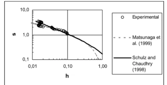
Figure 6. Comparison between the experimental h and the analytical solutions: f=1Hz, S=3cm, M=5.1cm, Section B.
0,01 0,10 1,00 10,00
0,01 0,10 1,00 10,00
h
s
Experimental
Matsunaga et al. (1999)
Schulz and Chaudhry (1998)
Figure 7. Comparison between the experimental h and the analytical solutions: f=1Hz, S=3cm, M=5.1cm, Section H.
0,1 1,0 10,0
0,001 0,010 0,100 1,000
h
s
Experimental
Matsunaga et al. (1999)
Schulz and Chaudhry (1998)
Figure 8. Comparison between the experimental h and the analytical solutions: f=2Hz, S=3cm, M=5.1cm, Section B.
0,1 1,0 10,0
0,01 0,10 1,00
h
s
Experimental
Matsunaga et al. (1999)
Schulz and Chaudhry (1998)
Conclusions
Experimental data for turbulent kinetic energy were generated using a grid immersed in water. The measurements were done using the Digital Particle Image Velocimetry, furnishing profiles of very good quality. The turbulent kinetic energy fields were analyzed
using solutions found in the literature, obtained with the k-ε
turbulence model. A comparison between experimental data and theoretical predictions was made. It is observed that the profiles generated by the analytical solutions agree, to a reasonable degree of
approximation, with those of the experimentalk data. Considering
the variations observed for the adjusted constants of the analytical solutions, it may be said that oscillating grid turbulence requires further investigation to confirm the analytical results.
Acknowledgements
The authors thank FAPESP, CAPES and CNPq (Brazil) for their support of this study, through grant # 520540/00.0 of CNPq and # 00/13953-6 of FAPESP.
References
Brumley, B.H. and Jirka, G.H., 1987, “Near-Surface Turbulence in a Grid-Stirred Tank”, Journal of Fluid Mechanics, Vol. 183, pp. 235-263.
Brunk, B., Shirk, M.W, Jensen, A., Jirka, G., and Lion, L.W., 1996, “Modeling Natural Hydrodynamics Systems With a Differential-Turbulence Column”, Journal of Hydraulic Engineering, Vol. 122, No. 7, pp. 373-380.
Cheng, C.Y., Atkinson, J.F., and Bursik, M.I., 1997, “Direct Measurement of Turbulence Structures in Mixing Jar Using PIV”, J. of Environmental Engineering, Vol. 123, No. 2, pp. 115-125.
Cheng, N.S. and Law, A.W.K., 2001, “Measurements of Turbulence Generated by Oscillating Grid”, Journal of Hydraulic Engineering, Vol. 127, No. 3, pp. 201-208.
Chu, C.R. and Jirka, G.H., 1992, “Turbulent Gas Flux Measurements Below the Air-Water Interface of a Grid-Stirred Tank”, J. Heat Mass Transfer, Vol. 35, No. 8, pp. 1957-1968.
De Silva, I.P.D. and Fernando, H.J.S., 1992, “Some Aspects of Mixing in a Stratified Turbulent Patch”, Journal of Fluid Mechanics, Vol. 240, pp. 601-625.
De Silva, I.P.D. and Fernando, H.J.S., 1994, “Oscillating Grids as a Source of Nearly Isotropic Turbulence”, Phys. Fluids, Vol. 6, pp. 2455-2464. Hopfinger, E.J. and Toly, J.A., 1976, “Spatially Decaying Turbulence and its Relation to Mixing Across Density Interfaces”, Journal of Fluid Mechanics, Vol. 78, pp. 155-175.
Janzen, J.G., 2003, “Detailment of the Turbulent Structure in Grid-Stirred Tanks” (In Portuguese), MSc.. Thesis, University of Sao Paulo, Sao Carlos, S.P., Brazil.
Matsunaga, N., Sugihara, Y., Komatsu, T. and Masuda, A., 1999, “Quantitative Properties of Oscillating-Grid Turbulence in a Homogeneous Fluid”, Fluid Dynamics Research, Vol. 25, pp. 147-165.
Medina, P., Sánchez, M.A. and Redondo, J.M., 2001, “Grid Stirred Turbulence: Applications to the Initiation of Sediment Motion and Lift-Off Studies”, Phys. Chem. Earth, Vol. 26, No. 4, pp. 299-304.
Nokes, R.I., 1988, “On the Entrainment Rate Across a Density Interface”, Journal of Fluid Mechanics, Vol. 188, pp. 185-204.
Quénot, G.M., Pakleza, T.A. and Kowalewski, T.A., 1998, “Particle Image Velocimetry with Optical Flow”, Experiments in Fluids, Vol. 25, pp. 177-189.
Rouse, H. and Dodu, J., 1955, “Diffusion Turbulente à Travers Une Discontinuité de Densité”, La Houille Blanche, No. 4, pp. 522-529.
Schulz, H.E. and Chaudhry, F.H., 1998, “Uma Aproximação para Turbulência Gerada por Grades Oscilantes”, Primeira Escola de Transição e Turbulência, COPPE, Anais, Vol I, pp.181-194.
Schulz, H.E. (2001), "Alternativas em Turbulência", Publicação EESC/USP, Editora RIMA, São Carlos, S.P., 143p.
Shy, S.S., Jang, R.H. and Tang, C.Y., 1996, “Simulation of Turbulent Burning Velocities Using Aqueous Autocatalytic Reactions in a Near-Homogeneous Turbulence”, Combust. Flame, Vol. 105, pp. 54-67.
Souza, L.B.S., 2002, “Study of the turbulent structure in flows generated by oscillating grids” (In Portuguese), MSc.. Thesis, University of Sao Paulo, Sao Carlos, S.P., Brazil.