Determinant factors of income inequality: evidence from a Portuguese region

(1)

(2)

1. Introduction

Income inequality is an important research area not only because of its impact on economic growth but also as support to economic policies that seek to reduce poverty and inequality (Fields, 2001). Research on this topic covers three main aspects: (i) methodological debate on how to measure inequality, (ii) quantification of the phenomenon in different countries/regions and periods, and (iii) identification of the determinants of inequality. In this study, we focus on this last feature, the least explored in economic literature.

The evaluation of the determinant factors of income inequality has been concretized through two main approaches: the traditional static inequality decomposition by income sources (Shorrocks, 1982) or by sub-groups (Shorrocks, 1984) and the regression-based inequality decomposition technique (Morduch and Sicular, 2002; Fields, 2003). The main purpose of this study is to propose a different methodology, based on a bilateral comparison of households, which allows a direct test through an econometric model of the determinant factors of income inequality.

The paper is organized as follows. Section 2 introduces the empirical methodology and presents the data. Section 3 summarizes the results. Section 4 concludes.

2. Empirical methodology

The traditional inequality decomposition approach proposed by Shorrocks (1982, 1984) has two important limitations. First, it has an eminently descriptive nature. Second, by construction the contribution(s) of the several characteristics of the household cannot be disentangled, and such knowledge may be important for economic policy (Naschold, 2009).

An important contribution to overcome these limitations is the regression-based inequality decomposition technique. This approach is a combination of income regression analysis and income source decomposition, allowing one to quantify how much inequality is explained by each income determinant.1

In this study, we propose an alternative approach. An important distinctive characteristic of this method is the fact that, instead of explaining the overall level of income inequality, it uses micro-data to analyze, in bilateral terms, the determinants of inequality. This is done through an econometric model in which a measure of inequality between each pair of households is regressed as a function of the variables that explain the degree of similarity/dissimilarity between households. The number of observations in the model corresponds therefore to the total number of pairs that can be obtained from the data. Since the measure of income inequality is the dependent variable, it becomes possible to directly assess the impact of alterations in each explanatory variable on inequality, giving a precise indication of how to minimize the inequalities identified. Additionally, if, for a given pair of households, we have information about all the explanatory variables included in the model, we can predict the level of income inequality between them.

Let us now briefly discuss the methodological options that need to be assumed before empirical analyses on income inequality. Specifically, the following aspects must

1

For examples of application of this methodology and discussion of their limitations, see, for instance, Wan and Zhou (2005) and Kimhi (2010).

(3)

be considered: (i) the indicator of resources, (ii) the demographic unit, and (iii) equivalence scales.

The indicator of resources most commonly used is the monetary disposable income, defined as the sum of work income, property income, pensions, other social transfers, and other private transfers after the deduction of the taxes on income and social contributions. However, this type of indicator excludes all forms of non-monetary income. In the current analysis, therefore, we use both monetary and total income. In this last case, the following items are also considered: the value of goods produced for own consumption, inputted rents, and remuneration in kind.

Regarding the demographic unit, following the widely accepted practice, we consider households.

A final issue that needs to be decided has to do with the comparison between unlike units. In fact, households with distinct compositions and dimensions require different incomes to achieve the same level of welfare. The use of equivalence scales allows calculating the household size in adult equivalents. In this study, we use the modified OECD scale, which gives a weight of 1 to the first adult, 0.5 to each of the remaining adults, and 0.3 for children under 14 years of age. When we divide the income (monetary and total) of each household by the number of equivalent adults, we obtain the adult equivalent income.

To measure income inequality between households i and h, we calculate:

       = = > + + − + = 0 if 0 0 if v h v i v h v i v h v i v h v h v i v i v h , i Y Y Y Y Y Y Y Y Y Y INEQ (1)

where v = {1, 2}, with 1 being monetary income, and 2 total income. Y expresses income per equivalent adult. INEQ is a relative measure of inequality and ranges between 0 (if the incomes of i and h are equal) and 1 (maximum inequality).

Regarding the way this variable is obtained, let us emphasize two aspects. First, since our focus is on the analysis of income inequality instead of poverty or richness,

INEQ is built to attend to the magnitude of the gap between the two households in terms of income, ignoring therefore which of them is the richest. For this reason, we assume the absolute value of the difference between the relative weights of each household in the total income of the two households under consideration. Obviously, if we wish to extend the evaluation to the connected concepts of poverty and richness, we could consider the difference without taking the absolute value.

Second, through the consideration of the denominator (Y_iv +Y_hv), we eliminate the sensibility of INEQ to the scale of measurement. A simple example illustrates this point. Let us consider four households (A, B, C, and D) with incomes Ya = 20, Yb = 40,

Yc = 1000, and Yd = 1020. If we consider as dependent variable hv v

i Y

Y − , the level of inequality between the pairs A-B and C-D is the same. However, while B has 100% more income than A, the household D has only 2% more income than C, reflecting a much smaller degree of inequality.

Since INEQ measures the level of inequality between two households, our explanatory variables are constructed in order to capture the differences between these

(4)

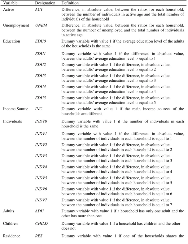
households in the dimensions that are relevant to explain income inequality. We consider four groups of variables, related to: (i) socio-economic characteristics of the household (ACT, UNEM, EDUC, and INC), (ii) composition and dimension of the household (INDV, ADU, and CHILD), (iii) the number of households in the residence - e.g., single or multiple-family dwelling (RES), and (iv) socio-economic characteristics of the individual of reference (LMS, GEND, and AGE).2 Table I presents the explanatory variables considered in the model.

Table I. Explanatory Variables

Variable Designation Definition

Active ACT Difference, in absolute value, between the ratios for each household,

between the number of individuals in active age and the total number of individuals of the household

Unemployment UNEM Difference, in absolute value, between the ratios for each household, between the number of unemployed and the total number of individuals in active age

Education EDU0 Dummy variable with value 1 if the average education level of the adults

of the households is the same

EDU1 Dummy variable with value 1 if the difference, in absolute value, between the adults’ average education level is equal to 1

EDU2 Dummy variable with value 1 if the difference, in absolute value,

between the adults’ average education level is equal to 2

Income Source INC Dummy variable with value 1 if the main income sources of the

households are different

Individuals INDV0 Dummy variable with value 1 if the number of individuals in each household is the same

INDV1 Dummy variable with value 1 if the difference, in absolute value, between the number of individuals in each household is equal to 1

Adults ADU Dummy variable with value 1 if a household has only one adult and the

other has more than one

Children CHILD Dummy variable with value 1 if a household has children and the other

does not

Residence RES Dummy variable with value 1 if one of the households shares the

2

The individual of reference of the household is the individual with the largest proportion of the annual net total income of the household.

(5)

residence and the other does not Labor Market

State

LMS Dummy variable with value 1 if the individuals of reference have different labor market states

Gender GEND Dummy variable with value 1 if the gender of the individual of reference

is different

Age AGE0 Dummy variable with value 1 if the individuals of reference belong to the same age group

AGE1 Dummy variable with value 1 if the absolute value of the difference between the age groups of the individuals of reference is equal to 1

Notes: (i) the construction of the group of variables related to age (AGE0 to AGE5) involves two steps. First, the age group of the individual of reference is identified: 1 (age between 18 and 24), 2 (25-29), 3 (30-44), 4 (45-64), 5 (65-74), and 6 (more than 74). Second, for each pair of households, we calculate the absolute value of the difference of the age groups of the individuals of reference; (ii) the construction of the dummy variables related to the comparison between the number of individuals (INDV0 to INDV7) is similar to the previous one. We start by identifying the number of individuals in each household and then calculate the difference in absolute terms between these numbers; (iii) the dummy variables related to households’ average education are obtained in three steps. First, the education level of each adult is identified: 1 (no education), 2 (primary education – 1st cycle), 3 (primary education – 2nd cycle), 4 (primary education – 3rd cycle), 5 (secondary education), and 6 (tertiary education). Second, for each household, the adults’ average education level is calculated. Finally, we compute, for each pair of households, the difference, in absolute value, between these average education levels. This difference is then rounded to the nearest unit.

When the dependent variable is bounded, using OLS regression may produce biased and inconsistent parameter estimates. One of the models that can be used instead, overcoming these problems, is the Tobit regression model (Tobin, 1958). Since INEQ varies between 0 and 1, meaning that the dependent variable of our model is bounded below and above, the two-limit Tobit regression is adequate (Rosett and Nelson, 1975).

Based on earlier evidence reported in the literature on poverty and inequality, the expected sign of the variables presented in Table I is positive, except for the case of: (i) the variables concerning the dimension and composition of the household, for which there is no obvious expected sign, and (ii) the variables related with the age of the individual of reference. In the latter case, the difficulty stems from the fact that higher incomes are usually concentrated in households with middle age individuals of reference while households with younger and older individuals of reference have, on average, lower incomes.

We use micro-data from the Office of National Statistics (INE) Household Budget Survey (IDEF) carried out in 2005/2006. Our sample includes the households residing in the region of Lisboa (1317 households).

3. Results

(6)

Table II. Determinant Factors of Income Inequality Explanatory variables Dependent variables INEQ1i,h INEQ 2 h , i ACT 0.019*** (13.35) 0.021*** (14.90) UNEM 0.028*** (24.32) 0.034*** (30.22) EDU1 0.012*** (12.73) 0.010*** (11.36) EDU2 0.045*** (48.00) 0.041*** (45.10) EDU3 0.103*** (105.66) 0.097*** (102.49) EDU4 0.191*** (177.23) 0.180*** (173.05) EDU5 0.306*** (189.46) 0.304*** (194.74) INC 0.015*** (24.95) -0.009*** (-15.88) INDV1 -0.002** (-2.86) -0.003*** (-4.70) INDV2 -0.001 (-0.91) -0.001** (-2.02) INDV3 0.0167*** (16.57) 0.0190*** (19.58) INDV4 0.0432*** (27.02) 0.0566*** (36.59) INDV5 0.039*** (14.08) 0.064*** (23.77) INDV6 0.058*** (12.63) 0.076*** (17.19) INDV7 0.049*** (5.18) 0.058*** (6.34) ADU -0.003*** (-5.05) -0.003*** (-5.63) CHILD -0.018*** (-30.07) -0.019*** (-31.64) RES 0.013*** (4.22) 0.014*** (4.78) LMS 0.002** (2.50) 0.004*** (6.48) GEND 0.007*** (13.50) 0.006*** (13.36) AGE1 -0.005*** (-8.00) -0.002*** (-3.34) AGE2 -0.011*** (-15.73) -0.005*** (-6.87) AGE3 -0.033*** (-33.95) -0.023*** (-25.15) AGE4 -0.048*** (-25.72) -0.035*** (-19.36) AGE5 -0.072*** (-20.56) -0.055*** (-16.11) CONSTANT 0.279*** (281.86) 0.277*** (289.24) Sigma 0.216*** (1316.25) 0.209*** (1316.46) Log-likelihood 96656.87 126071.28 Number of observations 866586 866586

Note: *, **, ***significant at 10%, 5% and 1%, respectively.

Regarding monetary income inequality, the results presented in Table II confirm the expected influence of variables related to the socio-economic characteristics of the household, i.e., the inequality increases: (i) with the difference between the number of individuals in active age in the total number of individuals of the households, (ii) with

(7)

the difference between the number of unemployed individuals in the total of active age individuals, (iii) with the difference between the average educational level of the adults of the households, and (iv) if the main sources of income are different. Among these effects, differences in terms of education are especially important to explain inequality. The evidence obtained is in accordance with earlier studies which have shown the importance of education levels as an important determinant of the labor market situation (Card, 1999). Individuals with higher levels of education are more likely to hold jobs that involve performing more complex tasks and that have better career perspectives and retirement plans. Additionally, they are more efficient in job searching (Arrow, 1997).

The impact of the variables related with the dimension and composition of the households is the most difficult to identify a priori. The evidence reveals that significant differences between households concerning the number of individuals that compose them, particularly when the difference is greater than three, tend to increase inequality. On the other hand, however, the variables ADU and CHILD have a negative impact on the level of income inequality. We should note that this result is not inconsistent with the evidence obtained from INDV because, while INDV is capturing quantitative differences in the dimension of the households, ADU and CHILD aim to provide some insights regarding their composition.

The variable related to the number of households in the residence confirms the expected sign. Thus, inequality is higher when we compare households in which one lives alone and the other shares the residence than when the number of households in the residence is the same.

When we consider the variables related to the individual of reference, the evidence suggests that inequality is higher when the gender of the individual of reference is different. This conclusion is clearly in line with theoretical and empirical research regarding the existence of important differences between genders in the labor market concerning, for instance, pay levels, promotions, and distribution across occupations (Altonji and Blank, 1999; Blau and Kahn, 2006). Discrimination behaviors from employers and co-workers, productivity differences, and differences in preferences, namely concerning competitive environments, are possible explanations for the less favorable situation of women. All these aspects have potential implications in terms of income, as shown, for instance, by De Silva (2008) for developing countries.

Additionally, confirming the expected impact, income inequality increases when the labor market states of the individuals of reference are different, as also suggested by the conclusions obtained by Moller et al. (2003).

A greater difference between the age of the individuals of reference is associated with lower inequality. Two reasons may explain this result. First, considering the distribution of the average income by the age of the individuals of reference, there is an inverted U shaped curve, in which households with a younger or older individual of reference have very similar incomes. Second, the middle-age group is, by far, the one where income dispersion is the greatest.

The evidence based on total income confirms the results obtained with monetary income, the only exception being INC, which now has a negative coefficient, indicating that households with different main sources of income have a lower degree of income inequality.

(8)

In this study we proposed a new approach for assessing the determinants of inequality in income distribution. This methodology, which is based on a bilateral comparison of income, was used to analyze inequality in the Portuguese region of Lisboa. The results show that inequality increases as a function of differences in: (i) the socio-economic characteristics of households (active age individuals, number of unemployed individuals, the main source of income, and average educational levels), (ii) aspects related to the dimension and composition of the household (number of individuals, adults, and children), (iii) the number of households in the residence, and (iv) the socio-economic characteristics of the individual of reference (gender, labor market state, and age). Considering all the variables, we also conclude that the largest impact on income inequality is caused by differences in terms of average education levels.

References

Altonji, J. and R. Blank (1999) “Race and gender in the labor market” in Handbook of

Labor Economics (vol. 3C) by O. Ashenfelter and D. Card, Eds., Amsterdam: North-Holland, 3143-3259.

Arrow, K. (1997) “The benefits of education and the formation of preferences” in The

social benefits of education by J. Behrman and N. Stacy, Eds., University of Michigan Press: Ann Arbor, 11-16.

Blau, F. and L. Kahn (2006) “The U.S. gender pay gap in the 1990s: slowing convergence” Industrial & Labor Relations Review 60, 45-66.

Card, D. (1999) “The causal effect of education on earnings” in Handbook of Labor

Economics (vol. 3A) by O. Ashenfelter and D. Card, Eds., Amsterdam: North-Holland, 1801-1863.

De Silva, I. (2008) “Micro-level determinants of poverty reduction in Sri Lanka: a multivariate approach” International Journal of Social Economics 35, 140-158.

Fields, G. (2001) Distribution and development: a new look at the developing world, Russell Sage Foundation: New York.

Fields, G. (2003) “Accounting for income inequality and its change: a new method, with application to the distribution of earnings in the United States” Research in Labour

Economics 22, 1-38.

Kimhi, A. (2010) “Jewish households, Arab households, and income inequality in rural Israel: ramifications for the Israeli-Arab conflict” Defence and Peace Economics 21, 381-394.

Moller, S., D. Bradley, E. Huber, F. Nielsen and J. Stephens (2003) “Determinants of relative poverty in advanced capitalist democracies” American Sociological Review 68, 22-51.

Morduch, J. and T. Sicular (2002) “Rethinking inequality decomposition with evidence from rural China” Economic Journal 112, 93-106.

(9)

Naschold, F. (2009) “Microeconomic determinants of income inequality in rural Pakistan” Journal of Development Studies 45, 746-768.

Rossett, R. and F. Nelson (1975) “Estimation of the two-limit Tobit regression model”

Econometrica 43, 141-146.

Shorrocks, A. (1982) “Inequality decomposition by factor component” Econometrica 50, 193-211.

Shorrocks, A. (1984) “Inequality decomposition by population subgroup” Econometrica 52, 1369-1385.

Tobin, J. (1958) “Estimation of relationships for limited depended variables”

Econometrica 26, 24-36.

Wan, G. and Z. Zhou (2005) “Income inequality in rural China: regression-based decomposition using household data” Review of Development Economics 9, 107-120.